Anisotropic geometry-conforming
d-simplicial meshing via isometric embeddings
The MIT Faculty has made this article openly available.
Please share
how this access benefits you. Your story matters.
Citation
Caplan, Philip Claude, et al. “Anisotropic Geometry-Conforming
d-Simplicial Meshing via Isometric Embeddings.” Procedia
Engineering, vol. 203, 2017, pp. 141–53. © 2017 The Authors
As Published
http://dx.doi.org/10.1016/J.PROENG.2017.09.798
Publisher
Elsevier BV
Version
Final published version
Citable link
http://hdl.handle.net/1721.1/115254
Terms of Use
Creative Commons Attribution-NonCommercial-NoDerivs License
ScienceDirect
Available online at www.sciencedirect.com
Procedia Engineering 203 (2017) 141–153
1877-7058 © 2017 The Authors. Published by Elsevier Ltd.
Peer-review under responsibility of the scientific committee of the 26th International Meshing Roundtable. 10.1016/j.proeng.2017.09.798
10.1016/j.proeng.2017.09.798
© 2017 The Authors. Published by Elsevier Ltd.
Peer-review under responsibility of the scientific committee of the 26th International Meshing Roundtable.
1877-7058 Available online at www.sciencedirect.com
Procedia Engineering 00 (2017) 000–000
www.elsevier.com/locate/procedia
26th International Meshing Roundtable, IMR26, 18-21 September 2017, Barcelona, Spain
Anisotropic geometry-conforming d-simplicial meshing
via isometric embeddings
Philip Claude Caplan, Robert Haimes, David L. Darmofal, Marshall C. Galbraith
Massachusetts Institute of Technology, 77 Massachusetts Ave., Cambridge 02139, USA
Abstract
We develop a dimension-independent, Delaunay-based anisotropic mesh generation algorithm suitable for integration with adap-tive numerical solvers. As such, the mesh produced by our algorithm conforms to an anisotropic metric prescribed by the solver as well as the domain geometry, given as a piecewise smooth complex. Motivated by the work of L´evy and Dassi [10–12,20], we use a discrete manifold embedding algorithm to transform the anisotropic problem to a uniform one. This work differs from previous approaches in several ways. First, the embedding algorithm is driven by a Riemannian metric field instead of the Gauss map, lending itself to general anisotropic mesh generation problems. Second we describe our method for computing restricted Voronoi diagrams in a dimension-independent manner which is used to compute constrained centroidal Voronoi tessellations. In particular, we compute restricted Voronoi simplices using exact arithmetic and use data structures based on convex polytope theory. Finally, since adaptive solvers require geometry-conforming meshes, we offer a Steiner vertex insertion algorithm for ensuring the extracted dual Delaunay triangulation is homeomorphic to the input geometries.
The two major contributions of this paper are: a method for isometrically embedding arbitrary mesh-metric pairs in higher dimensional Euclidean spaces and a dimension-independent vertex insertion algorithm for producing geometry-conforming Delau-nay meshes. The former is demonstrated on a two-dimensional anisotropic problem whereas the latter is demonstrated on both 3d and 4d problems.
c
2017 The Authors. Published by Elsevier Ltd.
Peer-review under responsibility of the scientific committee of the 26th International Meshing Roundtable.
Keywords: Anisotropic mesh generation, metric, Nash embedding theorem, isometric, geometry-conforming, restricted Voronoi diagram, constrained centroidal Voronoi tessellation, Steiner vertices, dimension-independent
1. Introduction
Adaptive numerical simulations have received considerable interest in the past decade [2]. Progress towards per-forming adaptive space-time simulations for time-dependent problems [38] demands algorithms for generating four-dimensional meshes and, though some work has been done in generating space-time Delaunay meshes by [16], the extension to the anisotropic case is an active area of research. As noted by Alauzet and Loseille in their study [2], the state-of-the-art in mesh adaptation is to first construct a metric field and subsequently generate a discrete mesh meant
E-mail address: pcaplan@mit.edu
1877-7058 c 2017 The Authors. Published by Elsevier Ltd.
Peer-review under responsibility of the scientific committee of the 26th International Meshing Roundtable. Available online at www.sciencedirect.com
Procedia Engineering 00 (2017) 000–000
www.elsevier.com/locate/procedia
26th International Meshing Roundtable, IMR26, 18-21 September 2017, Barcelona, Spain
Anisotropic geometry-conforming d-simplicial meshing
via isometric embeddings
Philip Claude Caplan, Robert Haimes, David L. Darmofal, Marshall C. Galbraith
Massachusetts Institute of Technology, 77 Massachusetts Ave., Cambridge 02139, USA
Abstract
We develop a dimension-independent, Delaunay-based anisotropic mesh generation algorithm suitable for integration with adap-tive numerical solvers. As such, the mesh produced by our algorithm conforms to an anisotropic metric prescribed by the solver as well as the domain geometry, given as a piecewise smooth complex. Motivated by the work of L´evy and Dassi [10–12,20], we use a discrete manifold embedding algorithm to transform the anisotropic problem to a uniform one. This work differs from previous approaches in several ways. First, the embedding algorithm is driven by a Riemannian metric field instead of the Gauss map, lending itself to general anisotropic mesh generation problems. Second we describe our method for computing restricted Voronoi diagrams in a dimension-independent manner which is used to compute constrained centroidal Voronoi tessellations. In particular, we compute restricted Voronoi simplices using exact arithmetic and use data structures based on convex polytope theory. Finally, since adaptive solvers require geometry-conforming meshes, we offer a Steiner vertex insertion algorithm for ensuring the extracted dual Delaunay triangulation is homeomorphic to the input geometries.
The two major contributions of this paper are: a method for isometrically embedding arbitrary mesh-metric pairs in higher dimensional Euclidean spaces and a dimension-independent vertex insertion algorithm for producing geometry-conforming Delau-nay meshes. The former is demonstrated on a two-dimensional anisotropic problem whereas the latter is demonstrated on both 3d and 4d problems.
c
2017 The Authors. Published by Elsevier Ltd.
Peer-review under responsibility of the scientific committee of the 26th International Meshing Roundtable.
Keywords: Anisotropic mesh generation, metric, Nash embedding theorem, isometric, geometry-conforming, restricted Voronoi diagram, constrained centroidal Voronoi tessellation, Steiner vertices, dimension-independent
1. Introduction
Adaptive numerical simulations have received considerable interest in the past decade [2]. Progress towards per-forming adaptive space-time simulations for time-dependent problems [38] demands algorithms for generating four-dimensional meshes and, though some work has been done in generating space-time Delaunay meshes by [16], the extension to the anisotropic case is an active area of research. As noted by Alauzet and Loseille in their study [2], the state-of-the-art in mesh adaptation is to first construct a metric field and subsequently generate a discrete mesh meant
E-mail address: pcaplan@mit.edu
1877-7058 c 2017 The Authors. Published by Elsevier Ltd.
to conform, in some sense, to this metric field. Whereas several algorithms (up to d = 3) exist for generating metric-conforming meshes, these edge-based [4,28] or cavity-based [24,25] operators are heuristic and do not extend easily to higher dimensions for producing four-dimensional meshes needed for adaptive space-time simulations. We there-fore pursue a mathematically rigorous dimension-independent approach since we believe the difficulties encountered when generating four-dimensional meshes are akin to those for higher dimensions.
The use of higher dimensional embeddings to generate anisotropic meshes has shown promise in recent years [10–12,20]. These efforts have focused on embedding surfaces to higher dimensional Euclidean spaces using either the normal vector of the surface [20] or the value and gradient of some approximated function [12]. These methods introduce a user-prescribed scaling factor on the codimension coordinates to magnify the amount of anisotropy and do not strive for isometric embeddings.
We focus on the requirements, from the mesh generation point-of-view, of an adaptive space-time numerical solver. We, therefore, expect the solver to provide us with a metric field and some description of the domain geometry - here, we restrict this description to piecewise smooth complexes (PSCs). Our work is motivated by the promising results associated with the use of high dimensional embeddings. Since the numerical solver expects a metric-conforming mesh upon termination of our meshing procedure, we develop an algorithm for isometrically embedding arbitrary mesh-metric pairs to high-dimensional spaces. This embedded mesh is then used to guide the isotropic mesh gen-eration problem in the embedding space. To generate the isotropic mesh, we use the constrained centroidal Voronoi tessellation, a variational Delaunay-based approach, since this simultaneously optimizes both the point distribution and topology of the isotropic mesh. Delaunay approaches are notorious for issues in conforming to domain boundaries and, though implementations exist for d = 2 and d = 3 in computing constrained Delaunay triangulations [31–36] or weighted Delaunay triangulations [7,8,13], their higher-dimensional extensions have yet to be implemented or demon-strated [33]. We therefore develop a Steiner vertex insertion algorithm applied to the restricted Voronoi diagram to conform to sharp features in an input geometry.
Notation
m(x) Riemannian metric field
Σij Mesh composed of i-polytopes with vertices embedded in Rj. κ i-simplex in any mesh Σijreferencing i + 1 vertices embedded in Rj
Vor(Z) Voronoi diagram generated by sites Z Vor(zi) Voronoi cell generated by sitezi
vorσ(Z) Voronoi diagram generated by sites Z restricted to some mesh σ = Σij, i.e. Vor(Z) ∩ σ
vorκ(zi) Voronoi cell generated by sitezirestricted to simplex κ, i.e. Vor(zi) ∩ κ
vorσ(zi) Voronoi cell generated by sitezirestricted to some mesh σ = Σij, i.e. Vor(zi) ∩ σ
note: vorσ(zi) = κ∈σvorκ(zi)
sym+
i i × i symmetric positive-definite tensor
2. Overall algorithm
The overall anisotropic boundary-conforming mesh generation algorithm is motivated by the work of L´evy and Dassi [10,11,20] in which surfaces were embedded to R6 using the Gauss map. After generating a uniform
dis-cretization along this embedded mesh, the vertices are mapped back by inverting the Gauss map. We follow a similar approach but compute the coordinates of the embedding using the prescribed metric tensor and extend the previous efforts to obtain geometry-conforming meshes in a dimension-independent manner. Specifically, the mesh generation algorithm follows the procedure outlined in Algorithm 1. The first stage consists of realizing the input mesh-metric pair as a submanifold of some higher-dimensional Euclidean space (Section 3). A unit tessellation is then generated along this embedded manifold (Section 4) from which we enforce geometry-conformity (Section 5). We work purely with the dual restricted Voronoi diagram and delay the extraction of the Delaunay mesh until we map the final mesh back to the original domain (Section 6). This work only deals with meshes whose topological dimension equals the physical dimension of the ambient space, d = j. As such, we drop the superscript and only write Σd instead of Σdd.
Philip Claude Caplan et al. / Procedia Engineering 203 (2017) 141–153 143 2 P. Caplan et al. / Procedia Engineering 00 (2017) 000–000
to conform, in some sense, to this metric field. Whereas several algorithms (up to d = 3) exist for generating metric-conforming meshes, these edge-based [4,28] or cavity-based [24,25] operators are heuristic and do not extend easily to higher dimensions for producing four-dimensional meshes needed for adaptive space-time simulations. We there-fore pursue a mathematically rigorous dimension-independent approach since we believe the difficulties encountered when generating four-dimensional meshes are akin to those for higher dimensions.
The use of higher dimensional embeddings to generate anisotropic meshes has shown promise in recent years [10–12,20]. These efforts have focused on embedding surfaces to higher dimensional Euclidean spaces using either the normal vector of the surface [20] or the value and gradient of some approximated function [12]. These methods introduce a user-prescribed scaling factor on the codimension coordinates to magnify the amount of anisotropy and do not strive for isometric embeddings.
We focus on the requirements, from the mesh generation point-of-view, of an adaptive space-time numerical solver. We, therefore, expect the solver to provide us with a metric field and some description of the domain geometry - here, we restrict this description to piecewise smooth complexes (PSCs). Our work is motivated by the promising results associated with the use of high dimensional embeddings. Since the numerical solver expects a metric-conforming mesh upon termination of our meshing procedure, we develop an algorithm for isometrically embedding arbitrary mesh-metric pairs to high-dimensional spaces. This embedded mesh is then used to guide the isotropic mesh gen-eration problem in the embedding space. To generate the isotropic mesh, we use the constrained centroidal Voronoi tessellation, a variational Delaunay-based approach, since this simultaneously optimizes both the point distribution and topology of the isotropic mesh. Delaunay approaches are notorious for issues in conforming to domain boundaries and, though implementations exist for d = 2 and d = 3 in computing constrained Delaunay triangulations [31–36] or weighted Delaunay triangulations [7,8,13], their higher-dimensional extensions have yet to be implemented or demon-strated [33]. We therefore develop a Steiner vertex insertion algorithm applied to the restricted Voronoi diagram to conform to sharp features in an input geometry.
Notation
m(x) Riemannian metric field
Σij Mesh composed of i-polytopes with vertices embedded in Rj. κ i-simplex in any mesh Σijreferencing i + 1 vertices embedded in Rj
Vor(Z) Voronoi diagram generated by sites Z Vor(zi) Voronoi cell generated by sitezi
vorσ(Z) Voronoi diagram generated by sites Z restricted to some mesh σ = Σij, i.e. Vor(Z) ∩ σ
vorκ(zi) Voronoi cell generated by sitezirestricted to simplex κ, i.e. Vor(zi) ∩ κ
vorσ(zi) Voronoi cell generated by sitezirestricted to some mesh σ = Σij, i.e. Vor(zi) ∩ σ
note: vorσ(zi) = κ∈σvorκ(zi)
sym+
i i × i symmetric positive-definite tensor
2. Overall algorithm
The overall anisotropic boundary-conforming mesh generation algorithm is motivated by the work of L´evy and Dassi [10,11,20] in which surfaces were embedded to R6 using the Gauss map. After generating a uniform
dis-cretization along this embedded mesh, the vertices are mapped back by inverting the Gauss map. We follow a similar approach but compute the coordinates of the embedding using the prescribed metric tensor and extend the previous efforts to obtain geometry-conforming meshes in a dimension-independent manner. Specifically, the mesh generation algorithm follows the procedure outlined in Algorithm 1. The first stage consists of realizing the input mesh-metric pair as a submanifold of some higher-dimensional Euclidean space (Section 3). A unit tessellation is then generated along this embedded manifold (Section 4) from which we enforce geometry-conformity (Section 5). We work purely with the dual restricted Voronoi diagram and delay the extraction of the Delaunay mesh until we map the final mesh back to the original domain (Section 6). This work only deals with meshes whose topological dimension equals the physical dimension of the ambient space, d = j. As such, we drop the superscript and only write Σd instead of Σdd.
The superscript on embedded meshes, however, is maintained.
P. Caplan et al. / Procedia Engineering 00 (2017) 000–000 3
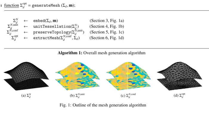
1 function Σoptd =generateMesh(Σd,m);
ΣNd ← embed(Σd,m) (Section 3, Fig. 1a)
ΣN,unitd ← unitTessellation(ΣNd) (Section 4, Fig. 1b)
ΣdN,conf ← preserveTopology(ΣN,unitd ) (Section 5, Fig. 1c)
Σoptd ← extractMesh(ΣdN,conf, Σd) (Section 6, Fig. 1d)
Algorithm 1: Overall mesh generation algorithm
(a) ΣN
d (b) ΣN,unitd (c) ΣN,confd (d) Σ
opt
d
Fig. 1: Outline of the mesh generation algorithm
2.1. Inputs
Input mesh. We restrict our attention to simplicial meshes or triangulations. The input d-simplicial mesh Σdis
de-scribed by a set of vertices and connectivities such that each simplex κ ∈ Σd references d + 1 vertices. The input
geometry whose topology must be preserved is additionally represented as a network of i-dimensional meshes Σij,
i ≤ d which are seen as piecewise smooth complexes (PSCs). For example, a volumetric mesh Σ3may have a network
of bounding surface meshes {Σ3
2} , curves {Σ31} and corners {Σ30} whose topology must be preserved.
Input metric. The input metric may be either the implied metric of the mesh, in which case all edges are of unit length
or some spatially continuous field of symmetric positive-definite tensors prescribed at the vertices of Σd. We compute
the length of every edge in the mesh using the geometric interpolation scheme of Alauzet [1].
2.2. Outputs
Output mesh. The algorithm produces a metric-conforming d-simplicial mesh Σoptd homeomorphic to the input mesh. Should Σd contain any submeshes, then Σoptd will also contain submeshes, each of which is homeomorphic to its
corresponding submesh of Σd.
Output metric. Along with the final mesh, the algorithm provides the edge lengths of the final mesh as measured
under the prescribed metric. Note that re-inputting this description of the metric into the algorithm would produce the same output mesh, the reasons for which will become apparent in the next section.
3. Computing the isometric embedding
Given a mesh Σd and Riemannian metricm(·) : x ∈ Σd → sym+d, our task is to compute the higher-dimensional
coordinates of the vertices of Σd. We leave the mesh connectivities untouched. Under the assumption the metric is
C0-continuous, the Nash embedding theorem [29] suggests (Σ,m) can be embedded into Rd+1.
In [10,11,20], the embedding coordinates are computed using the Gauss map, lifting the coordinates to R6 where
the codimension coordinates are computed by scaling the surface normals with a user-prescribed factor. The author in [12] similarly scales the value and gradient of an approximated function to compute the embedding. Our meshing
procedure is driven by an output-adaptive numerical solver and thus requests a mesh to conform to a prescribed metric. As such, our goal is to achieve the best possible isometry to match the requested metric and, since we are working with general d-dimensional meshes, we compute the embedding using a technique called multidimensional scaling.
Multidimensional scaling (MDS) is often used to infer a low-dimensional representation from high-dimensional data [5] using the restricted Euclidean metric. To this end, we remark on a deviation between our method and the true Nash embedding theorem since we now seek an embedding using the restricted Euclidean metric instead of the one induced by the Euclidean metric. The reason for this is a lack of a practical algorithm for realizing the Nash embedding theorem, despite efforts by Verma [37] and the nearly-isometric algorithm of McQueen [27].
Several techniques for MDS have been proposed, ranging from Isomap, Laplacian Eigenmaps, (non)-metric MDS all of which minimize a selected stress criteria [26]. Though the use of certain criteria, such as the Sammon mapping, achieve isometry better than others, we follow an approach called classical multidimensional scaling. This reduces to solving an eigenvalue problem for the embedding coordinates. The most important part of the embedding procedure is to ensure the map is bijective; loosely, the embedded mesh should not intersect itself. Instead of treating all coordi-nates as unknowns, we lift the mesh to a higher-dimensional space and simply compute the codimension coordicoordi-nates. Our method, outlined in Algorithm 2, is a variant of classical multidimensional scaling. The algorithm takes as input the mesh Σd, the metricm (either implied or prescribed) and the number of codimensions N0in which to embed. The
output is a nearly-isometric embedded mesh ΣN
d where N = d + N0. 1 function ΣNd =embed(Σd,m, N0); Input : Σd,m, N0 Output: ΣN d 2 E ← getEdges(Σd); 3 for e ∈ E do
4 e=metricLength(e,m) ; /* either implied or prescribed metric */
5 le=euclideanLength(e);
6 fe= e/le;
7 end
8 fmax← max({ fe}) ∀e ∈ E; 9 for e ∈ E do
10 G(e0,e1) ← fmax 2e− l2e; /* setup the graph adjacency matrix */
11 end
12 d = dijkstra(G) ; /* compute the geodesic length between every vertex */
13 D = d2; /* squared geodesic lengths */
14 B = −12JDJ ; /* where the centering matrix J = I − 11t/np */
/* and np is the number of vertices */ 15 (Q, Λ) = eig(B) ; /* eigendecomposition of B */
16 U0 =QN0Λ1/2N0 ; /* codimension coordinates using N0 largest */
/* eigenvalues and eigenvectors */
17 U = [X, U0/ fmax] ; /* lifting */
Algorithm 2: Embedding algorithm
Proposition 1. Algorithm 2 produces a bijective isometric embedding.
Proof. Even though the map producing the codimension coordinates may not be bijective, the lifting procedure is
bijective since each lifted point maps uniquely to a point in Σd. To show that our procedure preserves the metric edge
lengths, consider line 10. Following the lifting procedure, the squared length of the edges under the Euclidean metric are
Philip Claude Caplan et al. / Procedia Engineering 203 (2017) 141–153 145 4 P. Caplan et al. / Procedia Engineering 00 (2017) 000–000
procedure is driven by an output-adaptive numerical solver and thus requests a mesh to conform to a prescribed metric. As such, our goal is to achieve the best possible isometry to match the requested metric and, since we are working with general d-dimensional meshes, we compute the embedding using a technique called multidimensional scaling.
Multidimensional scaling (MDS) is often used to infer a low-dimensional representation from high-dimensional data [5] using the restricted Euclidean metric. To this end, we remark on a deviation between our method and the true Nash embedding theorem since we now seek an embedding using the restricted Euclidean metric instead of the one induced by the Euclidean metric. The reason for this is a lack of a practical algorithm for realizing the Nash embedding theorem, despite efforts by Verma [37] and the nearly-isometric algorithm of McQueen [27].
Several techniques for MDS have been proposed, ranging from Isomap, Laplacian Eigenmaps, (non)-metric MDS all of which minimize a selected stress criteria [26]. Though the use of certain criteria, such as the Sammon mapping, achieve isometry better than others, we follow an approach called classical multidimensional scaling. This reduces to solving an eigenvalue problem for the embedding coordinates. The most important part of the embedding procedure is to ensure the map is bijective; loosely, the embedded mesh should not intersect itself. Instead of treating all coordi-nates as unknowns, we lift the mesh to a higher-dimensional space and simply compute the codimension coordicoordi-nates. Our method, outlined in Algorithm 2, is a variant of classical multidimensional scaling. The algorithm takes as input the mesh Σd, the metricm (either implied or prescribed) and the number of codimensions N0in which to embed. The
output is a nearly-isometric embedded mesh ΣN
d where N = d + N0. 1 function ΣNd =embed(Σd,m, N0); Input : Σd,m, N0 Output: ΣN d 2 E ← getEdges(Σd); 3 for e ∈ E do
4 e=metricLength(e,m) ; /* either implied or prescribed metric */
5 le=euclideanLength(e);
6 fe= e/le;
7 end
8 fmax← max({ fe}) ∀e ∈ E; 9 for e ∈ E do
10 G(e0,e1) ← fmax 2e− l2e; /* setup the graph adjacency matrix */
11 end
12 d = dijkstra(G) ; /* compute the geodesic length between every vertex */
13 D = d2; /* squared geodesic lengths */
14 B = −12JDJ ; /* where the centering matrix J = I − 11t/np */
/* and np is the number of vertices */ 15 (Q, Λ) = eig(B) ; /* eigendecomposition of B */
16 U0=QN0Λ1/2N0 ; /* codimension coordinates using N0 largest */
/* eigenvalues and eigenvectors */
17 U = [X, U0/ fmax] ; /* lifting */
Algorithm 2: Embedding algorithm
Proposition 1. Algorithm 2 produces a bijective isometric embedding.
Proof. Even though the map producing the codimension coordinates may not be bijective, the lifting procedure is
bijective since each lifted point maps uniquely to a point in Σd. To show that our procedure preserves the metric edge
lengths, consider line 10. Following the lifting procedure, the squared length of the edges under the Euclidean metric are
||uj− ui||2=||xj− xi||2+||uj,0/ fmax− ui,0/ fmax||2. (1)
P. Caplan et al. / Procedia Engineering 00 (2017) 000–000 5
If the codimension coordinates exactly satisfy line 10, then under the restricted Euclidean metric,
||uj− ui||2=||xj− xi||2+fmax 2e/fmax− l2e= 2e, (2)
since ||xj− xi|| = le.
Although the minimum codimension needed to embed Σdis one, the advantage of embedding to higher
codimen-sions is clear since a greater number of eigenvalues will better approximate the disparity matrixB (line 15). In any case, the algorithm developed in the following sections for producing unit tessellations of embedded meshes is not computationally sensitive to the dimension of the Euclidean space.
4. Computing the unit tessellation Given an embedded mesh ΣN
d in some Euclidean space RN, our task is now to produce a unit tessellation of ΣNd. We
develop upon the work of L´evy and Bonneel [20] for computing constrained centroidal Voronoi tessellations (CCVTs) in a dimension-independent, topology-preserving manner. The main idea of the algorithm is to produce CCVTs of every embedded submesh of ΣN
d, here we employ Lloyd relaxation [23] for simplicity. The overall CCVT calculation
procedure is given in Algorithm 3.
1 function ΣdN,unit=unitTessellation(ΣdN); Input : ΣN
d
Output: ΣNunit d
2 Z ← ∅ ; /* initialize Delaunay seeds */
3 Σ← {ΣNj} ; /* accumulate all submeshes of ΣNd */
/* in increasing topological dimension */
4 for σ ∈ Σ do
5 vunit= j + 1/( j!√2j) ; /* σ has topological dimension j */ 6 vσ=volume(σ) ; /* compute volume of σ */
7 nσ= f vσ/vunit; /* f relates to the ideal vertex valency for j-simplices */
8 Zσ=randomSample(σ, nσ) ; /* randomly sample σ for nσ points */
9 Z ← [Z, Zσ]
10 while not converged do
11 compute vorσ(Z) ; /* restricted Voronoi diagram computation */ 12 compute centroids of vorσ(zi), ∀ zi∈ ZσprojectZσto σ.;
13 end
14 end
Algorithm 3: Computation of the centroidal Voronoi tessellation constrained to embedded meshes
Everything in Algorithm 3 is trivially dimension-independent except for the computation of the restricted Voronoi diagram (RVD). We therefore, discuss the specific data needed to compute RVDs in the following subsections.
4.1. Computing the restricted Voronoi diagram
The restricted Voronoi diagram can be defined in terms of restricted Voronoi simplices: vorσ(Z) =
κ∈σ
vorκ(Z). (3)
As such each vorκ(Z) can be computed independently, lending to a highly parallelizable algorithm. We implement the
of c++ kernel programming in OpenCL 2.1. Lines 11-12 can be replaced with a quasi-Newton approach as in [21,22], however we employ Lloyd relaxation [23] here for simplicity.
4.2. Computing restricted Voronoi simplices
Given a i-simplex κ ∈ Σij, vorκ(Z) can be computed by iteratively clipping κ against the Voronoi bisectors between
the Delaunay verticesZ. We additionally use the security radius theorem [20] to avoid unnecessary computations. Upon the first clip, we now deal with convex i-polytopes P = vorκ(zk) for some Delaunay seed (Voronoi cell)zk. To
apply the security radius theorem and additionally determine the geometry of P, we require the vertices (Vrep) of P. The clipping procedure iteratively introduces bisectors Π(zk,zr), providing the facets (Hrep) of P. Starting from
a i-simplex κ along with its i + 1 bounding (i − 1)-simplex facets, we immediately know the vertex-facet incidence matrix. Each Voronoi vertex arose due to a clip by a bisector Π(zk,zr) with an edge so we, in fact, know the
vertex-facet incidence matrix of each vertex at each step of the algorithm. Since Voronoi cells are simple polytopes, the vertex-facet incidence matrix provides the graph (edges) of P [18].
When a new vertex is created as the result of an intersection, it inherits the common bisectors between the endpoint vertices of the edge it lies on. We also track which mesh vertices in σ influence the intersection as well as which submeshes the vertices lie on. The former is critical for exactly querying the side of a point with respect to a bisector (see below) whereas the latter is important for preserving the topology of the output mesh, described in Section 5. The full clipping procedure is outlined in Algorithm 4.
4.3. Exact geometric predicates
Exact predicates are critical for the development of a robust mesh generator and are essential in our topology-preserving algorithm of the next section. We use the Predicate Construction Kit (PCK) developed by L´evy [19] to develop the predicates necessary for the generation of up to 4d meshes. The idea is similar to L´evy’s work and we refer the interested reader to his paper for further details. In particular, we have implemented the sided+1 predicate
for up to d = 4 and have tested the geometric exactness by placing the Delaunay seeds exactly at the Voronoi vertices generated by clipping against the Kuhn-Freudenthal triangulation in 4d. As mentioned earlier, each Voronoi vertex generated from the intersection of a Voronoi bisector with a polytope edge inherits the common vertices in κ from which they symbolically arise.
(a) Initial RVD (b) Final RVD after inserting vertices with our method
Fig. 2: Blocking facets in violation of P1 and how the vertex insertion method resolves the boundary. The background simplex edges are drawn to illustrate the insertion method. Voronoi cells with blocking facets are shown in pink.
5. Preserving the topology of the input geometry
This section describes how the topology of the input network of curves, surfaces, volumes, etc. is preserved in the output triangulation. Similar to the method where vertex-facet incidence relationships are tracked, vertices store the submeshes on which they lie. Upon the generation of a new Voronoi vertex, it inherits the common meshes between the endpoint vertices of the intersected edge that generated it. We preserve the topology by checking the two following properties:
(P1) Delaunay vertices are aware of which submesh they were seeded upon; denote this submesh as Σijfor a particular Delaunay vertexzk. All vertices for the Voronoi cell generated byzkshould lie on Σijor meshes that contain Σij
Philip Claude Caplan et al. / Procedia Engineering 203 (2017) 141–153 147 P. Caplan et al. / Procedia Engineering 00 (2017) 000–000 7
1 function vorκ(Z) = computeRVS (κ, Z);
Input : κ, Z Output: vorκ(Z)
2 DQ← closestPointToSimplex(κ) ; /* Delaunay queue starts with closest seed to a vertex of κ */
3 while DQ ∅ do
4 zk← pop(DQ) ; /* get next site in Delaunay queue */
5 P ← κ ; /* and add all facets of κ to the vertices they touch as ’bisectors’ */
6 r = 1 , zr← nearestNeighbour(zk,r) ; /* initial nearest neighbour */
7 while ||zr− zk|| ≤ 2||v − zk| ∀v ∈ Vrep(P) do 8 zr ← nearestNeighbour(zk,r); 9 Q = ∅; 10 V = Vrep(P); 11 for v ∈ V do 12 if side [v, Π(zk,zr)] > 0then 13 Q ← append(v); 14 end 15 end 16 E = graph(P); 17 for e ∈ E do
18 if side [e0, Π(zk,zr)] side [e1, Π(zk,zr)]then
19 Q ← append(e ∩ Π(zk,zr)) ; /* compute common bisectors, meshes & vertices of κ */
20 end
21 end
22 DQ← append(zr) ; /* add zr to Delaunay queue */ 23 r = r + 1 ; /* move to the next nearest neighbour */
24 P ← Q ; /* set P to the clipped polytope for future clippings */
25 end
26 end
Algorithm 4: Computation of a restricted Voronoi simplex
as a submesh; that is, for some other submesh Σljfor l > i. Should any vertex in the Voronoi cell lie on another submesh, the Delaunay site is said to block this submesh. This phenomenon is shown in Fig. 2a and Fig. 3a (see the green box over the right eye) in which Delaunay sites seeded on a 2-mesh block the 1-mesh boundaries from being connected. By connected, we mean for two sites to share an edge in the dual triangulation.
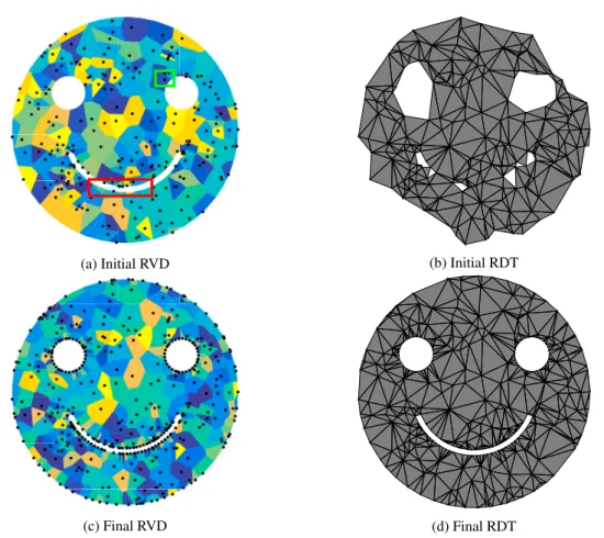
(P2) A Delaunay vertex seeded on some submesh Σij can equally block Σij from being connected in the dual De-launay triangulation. This is in fact a violation of the Topological Ball Property (TBP) [9] which states that every Voronoi cell should be homeomorphic to a closed topological ball. Violations of this property are bet-ter understood by examining the restricted Voronoi diagram of Fig. 3a (see the red box) in which Delaunay vertices seeded on the mouth contain connected components on both the upper and lower lips of the mouth. Several methods [7,8,13–15] which operate on the dual Delaunay triangulation have been proposed to identify violations of the TBP. Since we work purely with the restricted Voronoi diagram, violations of the TBP can be identified by aggregating each vorκ(zk) for a particular Delaunay seed vorκ(zk) and ensuring they are connected.
In other words, vorΣdN(zk) should form a closed topological ball.
For any vorκ(zk) violating the aforementioned properties, we identify the set of blocking facets which are formed
by the set of vertices of vorκ(zk) lying on any Σijthey block. Note the use of vorκ(zk) and not vorΣNd(zk) since the
the former is convex whereas the latter is not – an important property to ensure the facet is unblocked. Our method involves iteratively inserting Steiner vertices directly atzs = arg miny∈ f||y − zk|| which ultimately form part of the
triangulation of Σij. We do this iteratively since inserted points might themselves create Voronoi cells violating the above properties. Due to space limitations, the theory behind this selection along with our proof of termination using the Packing Lemma [9] will be given in future work.
As an example of the topology preservation algorithm, consider the input ge-ometry of the smile shown to the right. Random Delaunay seeds are placed at arbitrary locations within the domain; the reason for doing so is to test the robustness of the algorithm against even the most general cases. The initial RVD of Fig. 3a shows many vertices (in the red box) which vio-late the topological ball property. As such, the extracted restricted Delau-nay triangulation of Fig. 3b connects many of the vertices across the mouth in the input geometry. Following our vertex insertion procedure, the final RVD and topology-preserving RDT are shown in Figs. 3c and 3d, respec-tively.
(a) Initial RVD (b) Initial RDT
(c) Final RVD (d) Final RDT
Fig. 3: Demonstration of the topology preserving algorithm
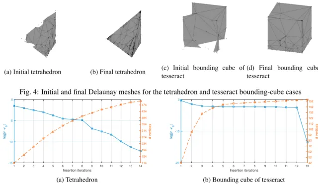
Now, let us demonstrate the topology-preserving aspect of the algorithm applied to three- and four-dimensional domains. We study a right-angled tetrahedron embedded in R3in which the prescribed boundaries are the 4 vertices,
6 edges and 4 bounding triangles of the tetrahedron. The initial Delaunay mesh with 114 random vertices is shown in Fig. 4a, which can be seen to omit several Delaunay vertices from the triangulation. After 14 iterations of our method, a boundary-conforming Delaunay triangulation is obtained, shown in Fig. 4b. The next case studied is the unit length tesseract embedded in R4. The geometry we wish to recover is the bounding cube of the tesseract located on the
Philip Claude Caplan et al. / Procedia Engineering 203 (2017) 141–153 149 P. Caplan et al. / Procedia Engineering 00 (2017) 000–000 9
(a) Initial tetrahedron (b) Final tetrahedron (c) Initial bounding cube oftesseract (d) Final bounding cube oftesseract
Fig. 4: Initial and final Delaunay meshes for the tetrahedron and tesseract bounding-cube cases
1 2 3 4 5 6 7 8 9 10 11 12 13 14 Insertion iterations -15 -10 -5 0 log|v -v 0 | 114 154 194 234 274 314 354 394 434 474 # vertices (a) Tetrahedron 1 2 3 4 5 6 7 8 9 10 11 12 13 Insertion iterations -20 -10 0 log|v -v 0 | 42 52 62 72 82 92 102 112 122 132 142 152 # vertices
(b) Bounding cube of tesseract
Fig. 5: Convergence of volume discrepancies for both the tetrahedron and tesseract bounding-cube cases condition of some space-time domain in 3d + t. 42 Delaunay seeds are initially randomly placed on the tesseract and boundary-conformity is achieved after 12 iterations, with the addition of 112 Steiner vertices. The initial and final meshes for the bounding cube are shown in Fig. 4c and 4d, respectively. Note that the initial Delaunay seeds were placed randomly; we are not interested in mesh quality or dihedral angles for these examples; we simply want to demonstrate that the boundary conformity algorithm correctly recovers the input geometry.
Fig. 5 shows the convergence of the number of Delaunay vertices along with the discrepancy in the volume between the current Delaunay triangulation restricted to the requested geometry and that of the target geometry itself – v0=1/6
for the tetrahedron and v0=1 for the bounding box of the tesseract – as the vertex insertion algorithm iterates. This
shows that both geometries require a significant number of vertices to preserve the topology of the input geometry. In general, the initial Delaunay vertices will be more judiciously placed as the result of some CVT iterations, however, our goal here is to demonstrate that, even in the presence of arbitrary vertex locations, the algorithm terminates and recovers the input geometry. Future work will investigate collapsing edges between the inserted vertices to achieve the desired simplex count.
6. Extracting the final mesh
After preserving the input mesh topology, the final mesh is extracted as the dual of the restricted Voronoi diagram. The coordinates of the vertices are mapped back to Rd by simply using the first d coordinates of the optimized
Delaunay seeds. We additionally note that the topology-preservation step involves several insertions. Our goal, at the current time, is to ensure the generated mesh conforms to a simplicial description of the input geometry and we will investigate a procedure by which edges between inserted vertices are collapsed to achieve the desired vertex density. The generated mesh would, however, no longer be a true Delaunay triangulation but some variant of the constrained Delaunay triangulation.
In essence this stage extracts the dual of an anisotropic Voronoi diagram and it is well-known that this dual may not be a triangulation (it may contain intersecting edges) [3,30]. We identify this as a current limitation of the Delaunay-based approach and restrict our attention to lower levels of anisotropy to ensure the dual is indeed a triangulation. Higher levels of anisotropy will be investigated in the future and methods for extracting the dual triangulation will be developed. We remark on some possible solutions in the results below.
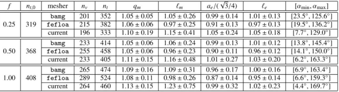
f nt,0 mesher nv nt qm m ae/(√3/4) e [αmin, αmax] 0.25 319 bamg 201 352 1.05 ± 0.05 1.05 ± 0.26 0.99 ± 0.14 1.01 ± 0.13 [23.5◦,125.6◦] fefloa 215 382 1.06 ± 0.06 0.97 ± 0.25 0.91 ± 0.13 0.97 ± 0.13 [19.5◦,136.2◦] current 196 333 1.10 ± 0.19 1.15 ± 0.41 1.05 ± 0.24 1.05 ± 0.18 [7.7◦,129.0◦] 0.50 368 bamg 233 414 1.05 ± 0.06 1.06 ± 0.24 0.99 ± 0.13 1.01 ± 0.12 [13.8◦,145.4◦] fefloa 255 458 1.05 ± 0.06 0.96 ± 0.23 0.90 ± 0.11 0.96 ± 0.12 [14.1◦,150.0◦] current 233 405 1.11 ± 0.15 1.16 ± 0.48 1.01 ± 0.27 1.03 ± 0.20 [6.2◦,163.3◦] 1.00 408 bamg 265 474 1.09 ± 0.16 1.09 ± 0.31 0.96 ± 0.17 1.00 ± 0.16 [6.9 ◦,163.4◦] fefloa 289 524 1.08 ± 0.11 0.98 ± 0.26 0.87 ± 0.14 0.95 ± 0.14 [6.6◦,159.3◦] current 264 460 1.13 ± 0.15 1.23 ± 0.75 0.99 ± 0.32 1.02 ± 0.23 [4.4◦,169.7◦]
Table 1: Expected number of triangles (nt,0), number of vertices (nv) and triangles (nt) with average and standard
deviation for metric quality (qm), metric lengths ( m), normalized embedded area (ae), embedded length ( e) and angle
ranges [αmin, αmax] for meshers conforming to the metric induced by Eq. (4).
7. Comparison with existing anisotropic two-dimensional mesh generators
In this section we compare the developed algorithm with existing anisotropic mesh generation technologies, namely bamg[17] and fefloa [24,25]. The former uses a metric-based version of the Delaunay criterion whereas the latter employs a local cavity-based approach. Comparisons with three-dimensional mesh generators will follow in future work. Each of the three algorithms requires an input background mesh and a description of the metric field at the vertices of this mesh. The first metric field chosen in this study is taken as the induced metric of the following surface: u(x) = x, y, z(x, y) , z(x, y) = 5 tanh f · (y − cos(πx/5) + 5) , [x, y] ∈ Ω = [0, 10]2. (4) In other words,m(x) = ∇ut∇u. We sweep through the parameter f to vary the level of anisotropy in the problem.
The initial mesh is taken as the output of the algorithm described in [6] which uses node movement, edges splits, collapses and swaps to conform to the input analytic metric field. For each level of anisotropy, we obtain the mesh generated from all three algorithms and re-embed the generated two-dimensional vertices into three dimensions using the surface in Eq. (4). Although it differs from the discrete embedding obtained from Algorithm 2, it provides a means for comparing the three algorithms. In particular we measure the metric quality as qm = 2m,rms/(4√3am) ∈
[1, ∞] where m,rmsis the root-mean-square of the three edge lengths of a triangle and amis the area, both of which
are measured under the analytic metric. The normalization factor of 4√3 is used to assign a unit quality to the ideal triangle. We also show the average and standard deviations for the metric edge lengths ( m) as well as the
Euclidean areas (ae) and Euclidean edge lengths ( e) as measured after re-embedding the meshes with the analytic
embedding. In the context of generating a unit mesh for an adaptive numerical solver, the average Euclidean area should be close to √3/4 and the Euclidean edge lengths should be 1. The expected number of triangles can be computed by dividing the area of the analytic surface by the area of a unit equilateral triangle which comes out to
nt,0=(4/√3) Ω
1 + (∂z/∂x)2+(∂z/∂y)2dxdy.
The results, tabulated in Table 1, indicate that our algorithm gives good areas (ae) and edge lengths ( e) under the
Euclidean metric but is slightly outperformed by existing technologies for the measures of metric quality (qm) and
metric edge lengths ( m). However, observe that the number of triangles generated by our algorithm (nt) is closer to
the expected number (nt,0) for all f . The minimum and maximum angles for the meshes generated by all algorithms
are reasonable.
For reference, the mesh generated by our algorithm is shown in Fig. 6 for the case with f = 1.0. We show the optimized restricted Delaunay triangulation after boundary conformity has been imposed (Fig. 6a), the anisotropic restricted Delaunay triangulation after mapping back to R2 (Fig. 6b) and the re-embedded mesh using the lifting
described in Eq. (4) (Fig. 6c). The mesh in Fig. 6a is different than the mesh in Fig. 6c because the restricted Euclidean metric was used to compute the embedding.
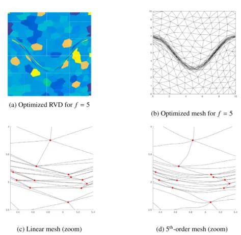
As mentioned in Section 6, the dual of an anisotropic Voronoi diagram may not be a triangulation due to the phenomenon remarked upon by [3,30]. Although all the meshes presented earlier were verified (by checking the total volume of the generated mesh) to be valid triangulations, this phenomenon was observed at higher f . The mesh generated by our algorithm for f = 5 is shown in Fig. 7b and the self-intersecting edges are shown in the zoomed
Philip Claude Caplan et al. / Procedia Engineering 203 (2017) 141–153 151 10 P. Caplan et al. / Procedia Engineering 00 (2017) 000–000
f nt,0 mesher nv nt qm m ae/(√3/4) e [αmin, αmax]
0.25 319 bamg 201 352 1.05 ± 0.05 1.05 ± 0.26 0.99 ± 0.14 1.01 ± 0.13 [23.5◦,125.6◦] fefloa 215 382 1.06 ± 0.06 0.97 ± 0.25 0.91 ± 0.13 0.97 ± 0.13 [19.5◦,136.2◦] current 196 333 1.10 ± 0.19 1.15 ± 0.41 1.05 ± 0.24 1.05 ± 0.18 [7.7◦,129.0◦] 0.50 368 bamg 233 414 1.05 ± 0.06 1.06 ± 0.24 0.99 ± 0.13 1.01 ± 0.12 [13.8◦,145.4◦] fefloa 255 458 1.05 ± 0.06 0.96 ± 0.23 0.90 ± 0.11 0.96 ± 0.12 [14.1◦,150.0◦] current 233 405 1.11 ± 0.15 1.16 ± 0.48 1.01 ± 0.27 1.03 ± 0.20 [6.2◦,163.3◦] 1.00 408 bamg 265 474 1.09 ± 0.16 1.09 ± 0.31 0.96 ± 0.17 1.00 ± 0.16 [6.9 ◦,163.4◦] fefloa 289 524 1.08 ± 0.11 0.98 ± 0.26 0.87 ± 0.14 0.95 ± 0.14 [6.6◦,159.3◦] current 264 460 1.13 ± 0.15 1.23 ± 0.75 0.99 ± 0.32 1.02 ± 0.23 [4.4◦,169.7◦]
Table 1: Expected number of triangles (nt,0), number of vertices (nv) and triangles (nt) with average and standard
deviation for metric quality (qm), metric lengths ( m), normalized embedded area (ae), embedded length ( e) and angle
ranges [αmin, αmax] for meshers conforming to the metric induced by Eq. (4).
7. Comparison with existing anisotropic two-dimensional mesh generators
In this section we compare the developed algorithm with existing anisotropic mesh generation technologies, namely bamg[17] and fefloa [24,25]. The former uses a metric-based version of the Delaunay criterion whereas the latter employs a local cavity-based approach. Comparisons with three-dimensional mesh generators will follow in future work. Each of the three algorithms requires an input background mesh and a description of the metric field at the vertices of this mesh. The first metric field chosen in this study is taken as the induced metric of the following surface: u(x) = x, y, z(x, y) , z(x, y) = 5 tanh f · (y − cos(πx/5) + 5) , [x, y] ∈ Ω = [0, 10]2. (4) In other words,m(x) = ∇ut∇u. We sweep through the parameter f to vary the level of anisotropy in the problem.
The initial mesh is taken as the output of the algorithm described in [6] which uses node movement, edges splits, collapses and swaps to conform to the input analytic metric field. For each level of anisotropy, we obtain the mesh generated from all three algorithms and re-embed the generated two-dimensional vertices into three dimensions using the surface in Eq. (4). Although it differs from the discrete embedding obtained from Algorithm 2, it provides a means for comparing the three algorithms. In particular we measure the metric quality as qm = 2m,rms/(4√3am) ∈
[1, ∞] where m,rmsis the root-mean-square of the three edge lengths of a triangle and amis the area, both of which
are measured under the analytic metric. The normalization factor of 4√3 is used to assign a unit quality to the ideal triangle. We also show the average and standard deviations for the metric edge lengths ( m) as well as the
Euclidean areas (ae) and Euclidean edge lengths ( e) as measured after re-embedding the meshes with the analytic
embedding. In the context of generating a unit mesh for an adaptive numerical solver, the average Euclidean area should be close to √3/4 and the Euclidean edge lengths should be 1. The expected number of triangles can be computed by dividing the area of the analytic surface by the area of a unit equilateral triangle which comes out to
nt,0=(4/√3) Ω
1 + (∂z/∂x)2+(∂z/∂y)2dxdy.
The results, tabulated in Table 1, indicate that our algorithm gives good areas (ae) and edge lengths ( e) under the
Euclidean metric but is slightly outperformed by existing technologies for the measures of metric quality (qm) and
metric edge lengths ( m). However, observe that the number of triangles generated by our algorithm (nt) is closer to
the expected number (nt,0) for all f . The minimum and maximum angles for the meshes generated by all algorithms
are reasonable.
For reference, the mesh generated by our algorithm is shown in Fig. 6 for the case with f = 1.0. We show the optimized restricted Delaunay triangulation after boundary conformity has been imposed (Fig. 6a), the anisotropic restricted Delaunay triangulation after mapping back to R2 (Fig. 6b) and the re-embedded mesh using the lifting
described in Eq. (4) (Fig. 6c). The mesh in Fig. 6a is different than the mesh in Fig. 6c because the restricted Euclidean metric was used to compute the embedding.
As mentioned in Section 6, the dual of an anisotropic Voronoi diagram may not be a triangulation due to the phenomenon remarked upon by [3,30]. Although all the meshes presented earlier were verified (by checking the total volume of the generated mesh) to be valid triangulations, this phenomenon was observed at higher f . The mesh generated by our algorithm for f = 5 is shown in Fig. 7b and the self-intersecting edges are shown in the zoomed
P. Caplan et al. / Procedia Engineering 00 (2017) 000–000 11
(a) Optimized embedded mesh (b) Optimized mesh (c) Re-embedded optimized mesh
Fig. 6: Meshes generated by our algorithm for the metric induced by Eq. (4) with f = 1.0
(a) Optimized RVD for f = 5
(b) Optimized mesh for f = 5
(c) Linear mesh (zoom) (d) 5th-order mesh (zoom)
Fig. 7: Extracting the fifth-order dual of the anisotropic Voronoi diagram for the metric induced by Eq. (4) with f = 5 section of Fig. 7c. Note that the Delaunay seeds are marked with red dots to make the self-intersections evident. One possible solution is to instead introduce equally spaced high-order nodes on the dual Delaunay edges and project them to the original embedded manifold. In so doing, this ensures the high-order representation contains edges on the embedded manifold which we know is one-to-one by the embedding procedure of Algorithm 2. A fifth-order representation of the same section of Fig. 7c is shown in Fig. 7d which appears free of intersecting triangles. This idea of extracting a curved Delaunay triangulation from a curved anisotropic Voronoi diagram seems promising and will be investigated in the future.
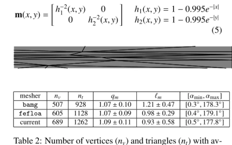
Next, we examine the ability of the algorithm to handle higher levels of anisotropy. We choose the metric given by Eq. (5) in a domain (x, y) ∈ Ω = [−5, 5]2, which exhibits a maximum anisotropy ratio of nearly 200:1 and the
number of triangles should equal 980. Note this example does not introduce inverted triangles after extracting the Delaunay triangulation from the anisotropic Voronoi diagram, as observed earlier. Again, we compare the developed algorithm with bamg and fefloa and tabulate the results in Table 2. Since this metric was not derived from an
ana-lytic surface, we cannot re-embed the meshes and assess ae and eas in the previous example. In addition, we use
a four-dimensional Euclidean space to embed the mesh-metric pair. bamg and fefloa more closely achieve a unit metric quality but we note that our algorithm still performs well in achieving unit metric edge lengths. All algorithms generate meshes with both large and small angles and whereas bamg undershoots the number of triangles, both our algorithm and fefloa overshoot nt,0. The optimized mesh generated by our algorithm is shown in Fig. 8.
Fig. 8: Mesh generated by our algorithm for the metric of Eq. (5). Zoomed portion of red box on the right. m(x, y) = h−2 1 (x, y) 0 0 h−2 2 (x, y) h1(x, y) = 1 − 0.995e−|x| h2(x, y) = 1 − 0.995e−|y| (5)
mesher nv nt qm m [αmin, αmax]
bamg 507 928 1.07 ± 0.10 1.21 ± 0.47 [0.3◦,178.3◦]
fefloa 605 1128 1.07 ± 0.09 0.98 ± 0.29 [0.4◦,179.1◦]
current 689 1262 1.09 ± 0.11 0.93 ± 0.58 [0.5◦,177.8◦]
Table 2: Number of vertices (nv) and triangles (nt) with
av-erage and standard deviation for metric quality (qm), metric
lengths ( m) and angle ranges [αmin, αmax] for the metric of
Eq. (5).
8. Conclusions
This work developed a new theoretical framework and algorithm for generating anisotropic geometry-conforming Delaunay meshes in a dimension-independent manner. Motivated by space-time adaptive numerical solvers, we aim to conform to a requested metric as well as an input geometry. The first contribution is a method for isometrically embedding mesh-metric pairs into higher-dimensional Euclidean spaces using multidimensional scaling and guaran-teeing the embedding is one-to-one. New mesh vertices are then optimized along the embedded manifold using the centroidal Voronoi tessellation. We provide a dimension-independent algorithm for computing this along with the restricted Voronoi diagram. Finally, the topology of the input geometry is preserved using an algorithm for inserting Steiner vertices along the input geometry and was demonstrated – our proof will follow in the future – to converge on some simple three- and four-dimensional geometries.
Future work
From the theoretical side, there are still some improvements that can be done in extracting the final Delaunay mesh topology since simplices may be inverted despite the embedding being one-to-one. Though this is well-known to occur when extracting the dual of anisotropic Voronoi diagrams, we suggest a solution in which the extracted Delaunay edges are instead curved where the high-order nodes are computed by projecting them to the embedded mesh, thus ensuring the extracted mesh is valid. Generating curvilinear meshes is desirable for high-order solvers and we will therefore investigate this idea in the future. We also plan to investigate alternative topologies in situations where the solver demands a straight-sided mesh. Our geometry-conforming algorithm tends to insert a large number of vertices into the triangulation. One option to obtain the desired vertex and simplex density in the resulting mesh is to revisit these inserted vertices and collapse edges between them.
References
[1] Fr´ed´eric Alauzet. Size gradation control of anisotropic meshes. Finite Elem. Anal. Des., 46(1-2):181–202, January 2010.
[2] Fr´ed´eric Alauzet and Adrien Loseille. A decade of progress on anisotropic mesh adaptation for computational fluid dynamics. Comput. Aided
Philip Claude Caplan et al. / Procedia Engineering 203 (2017) 141–153 153 12 P. Caplan et al. / Procedia Engineering 00 (2017) 000–000
lytic surface, we cannot re-embed the meshes and assess aeand eas in the previous example. In addition, we use
a four-dimensional Euclidean space to embed the mesh-metric pair. bamg and fefloa more closely achieve a unit metric quality but we note that our algorithm still performs well in achieving unit metric edge lengths. All algorithms generate meshes with both large and small angles and whereas bamg undershoots the number of triangles, both our algorithm and fefloa overshoot nt,0. The optimized mesh generated by our algorithm is shown in Fig. 8.
Fig. 8: Mesh generated by our algorithm for the metric of Eq. (5). Zoomed portion of red box on the right. m(x, y) = h−2 1 (x, y) 0 0 h−2 2 (x, y) h1(x, y) = 1 − 0.995e−|x| h2(x, y) = 1 − 0.995e−|y| (5)
mesher nv nt qm m [αmin, αmax]
bamg 507 928 1.07 ± 0.10 1.21 ± 0.47 [0.3◦,178.3◦]
fefloa 605 1128 1.07 ± 0.09 0.98 ± 0.29 [0.4◦,179.1◦]
current 689 1262 1.09 ± 0.11 0.93 ± 0.58 [0.5◦,177.8◦]
Table 2: Number of vertices (nv) and triangles (nt) with
av-erage and standard deviation for metric quality (qm), metric
lengths ( m) and angle ranges [αmin, αmax] for the metric of
Eq. (5).
8. Conclusions
This work developed a new theoretical framework and algorithm for generating anisotropic geometry-conforming Delaunay meshes in a dimension-independent manner. Motivated by space-time adaptive numerical solvers, we aim to conform to a requested metric as well as an input geometry. The first contribution is a method for isometrically embedding mesh-metric pairs into higher-dimensional Euclidean spaces using multidimensional scaling and guaran-teeing the embedding is one-to-one. New mesh vertices are then optimized along the embedded manifold using the centroidal Voronoi tessellation. We provide a dimension-independent algorithm for computing this along with the restricted Voronoi diagram. Finally, the topology of the input geometry is preserved using an algorithm for inserting Steiner vertices along the input geometry and was demonstrated – our proof will follow in the future – to converge on some simple three- and four-dimensional geometries.
Future work
From the theoretical side, there are still some improvements that can be done in extracting the final Delaunay mesh topology since simplices may be inverted despite the embedding being one-to-one. Though this is well-known to occur when extracting the dual of anisotropic Voronoi diagrams, we suggest a solution in which the extracted Delaunay edges are instead curved where the high-order nodes are computed by projecting them to the embedded mesh, thus ensuring the extracted mesh is valid. Generating curvilinear meshes is desirable for high-order solvers and we will therefore investigate this idea in the future. We also plan to investigate alternative topologies in situations where the solver demands a straight-sided mesh. Our geometry-conforming algorithm tends to insert a large number of vertices into the triangulation. One option to obtain the desired vertex and simplex density in the resulting mesh is to revisit these inserted vertices and collapse edges between them.
References
[1] Fr´ed´eric Alauzet. Size gradation control of anisotropic meshes. Finite Elem. Anal. Des., 46(1-2):181–202, January 2010.
[2] Fr´ed´eric Alauzet and Adrien Loseille. A decade of progress on anisotropic mesh adaptation for computational fluid dynamics. Comput. Aided
Des., 72(C):13–39, March 2016.
P. Caplan et al. / Procedia Engineering 00 (2017) 000–000 13 [3] Jean-Daniel Boissonnat, Ramsay Dyer, Arijit Ghosh, and Nikolay Martynchuk. An obstruction to Delaunay triangulations in Riemannian
manifolds. arXiv preprint arXiv:1612.02905, 2016.
[4] Houman Borouchaki and Pascal J. Frey. Adaptive triangular-quadrilateral mesh generation. Intl. J. Numer. Methods Eng, pages 915–934, 1998. [5] Alexander M. Bronstein, Michael M. Bronstein, and Ron Kimmel. Numerical Geometry of Non-Rigid Shapes. Springer Monographs in
Computer Science, 2009.
[6] Philip C. Caplan. An adaptive framework for high-order, mixed-element numerical simulations. Master’s thesis, Mass. Inst. of Tech., Depart-ment of Aeronautics and Astronautics, June 2014.
[7] Siu-Wing Cheng, Tamal K. Dey, and Joshua A. Levine. A Practical Delaunay Meshing Algorithm for a Large Class of Domains, pages 477–494. Springer Berlin Heidelberg, Berlin, Heidelberg, 2008.
[8] Siu-Wing Cheng, Tamal K. Dey, and Edgar A. Ramos. Delaunay refinement for piecewise smooth complexes. In Proc. 18th Annu. ACM-SIAM
Sympos. Discrete Algorithms, pages 1096–1105. ACM Press, 2007.
[9] Siu-Wing Cheng, Tamal K. Dey, and Jonathan Shewchuk. Delaunay Mesh Generation. Chapman & Hall/CRC, 1st edition, 2012.
[10] Franco Dassi, Patricio Farrell, and Hang Si. An anisoptropic surface remeshing strategy combining higher dimensional embedding with radial basis functions. Procedia Engineering, 163:72 – 83, 2016. 25th International Meshing Roundtable.
[11] Franco Dassi, Andrea Mola, and Hang Si. Curvature-adapted remeshing of CAD surfaces. Procedia Engineering, 82:253 – 265, 2014. [12] Franco Dassi, Hang Si, Simona Perotto, and Timo Streckenbach. Anisotropic finite element mesh adaptation via higher dimensional embedding.
Procedia Engineering, 124:265 – 277, 2015.
[13] Tamal K Dey and Andrew G Slatton. Localized Delaunay refinement for volumes. Computer Graphics Forum, 30(5):1417–1426, 2011. [14] Darren Engwirda. Voronoi-based point-placement for three-dimensional Delaunay-refinement. Procedia Engineering, 124:330 – 342, 2015. [15] Darren Engwirda. Conforming restricted Delaunay mesh generation for piecewise smooth complexes. Procedia Engineering, 163:84 – 96,
2016.
[16] Panagiotis Foteinos and Nikos Chrisochoides. 4d space-time Delaunay meshing for medical images. Proc. of the 22nd International Meshing Roundtable, 2014.
[17] Fr´ed´eric Hecht. Bamg: Bidimensional anisotropic mesh generator, 1998. http://www-rocq1.inria.fr/gamma/cdrom/www/bamg/eng.htm.
[18] Martin Henk, J¨urgen Richter-Gebert, and G¨unter M. Ziegler. Basic properties of convex polytopes. In Handbook of Discrete and Computational
Geometry, 2nd Ed., 2004.
[19] Bruno L´evy. Robustness and efficiency of geometric programs: The predicate construction kit. Computer-Aided Design, 72:3–12, 2016. [20] Bruno L´evy and Nicolas Bonneel. Variational anisotropic surface meshing with Voronoi parallel linear enumeration. In Proceedings of the
International Meshing Roundtable, 2012.
[21] Bruno L´evy and Yang Liu. Lpcentroidal Voronoi tessellation and its applications. ACM Transactions on Graphics (SIGGRAPH conference
proceedings), 2010.
[22] Yang Liu, Wenping Wang, Bruno L´evy, Feng Sun, Dong Ming Yan, Lin Lu, and Chenglei Yang. On centroidal Voronoi tessellation - energy smoothness and fast computation. Technical report, Hong-Kong University and INRIA - ALICE Project Team, 2008.
[23] Stuart P. Lloyd. Least squares quantization in PCM. IEEE Transaction on Information Theory, IT-28(2):129–137, 1982. [24] Adrien Loseille. Metric-orthogonal anisotropic mesh generation. Procedia Engineering, 82:403 – 415, 2014.
[25] Adrien Loseille and Rainald L¨ohner. Cavity-Based Operators for Mesh Adaptation. In American Institute of Aeronautics and Astronautics, ed-itors, 51st AIAA Aerospace Sciences Meeting including the New Horizons Forum and Aerospace Exposition. American Institute of Aeronautics and Astronautics, 2013.
[26] Laurens Van Der Maaten, Eric Postma, and Jaap Van Den Herik. Dimensionality reduction: A comparative review. Technical report, Tilburg University Center for Creative Computing, 2009.
[27] James McQueen, Marina Meila, and Dominique Joncas. Nearly isometric embedding by relaxation. In D. D. Lee, M. Sugiyama, U. V. Luxburg, I. Guyon, and R. Garnett, editors, Advances in Neural Information Processing Systems 29, pages 2631–2639. Curran Associates, Inc., 2016. [28] Todd Michal and Joshua Krakos. Anisotropic mesh adaptation through edge primitive operations. AIAA 2012-159, 2012.
[29] John F. Nash. C1isometric imbeddings. Annals of Mathematics, 60:383–396, November 1954.
[30] Mael Rouxel-Labb´e. Anisotropic mesh generation. PhD dissertation, University´e Cˆote d’Azur, 2016.
[31] Jonathan Richard Shewchuk. A condition guaranteeing the existence of higher-dimensional constrained Delaunay triangulations. In
Proceed-ings of the Fourteenth Annual Symposium on Computational Geometry, SCG ’98, pages 76–85, New York, NY, USA, 1998. ACM.
[32] Jonathan Richard Shewchuk. Constrained Delaunay tetrahedralizations and provably good boundary recovery. In In Eleventh International
Meshing Roundtable, pages 193–204, 2002.
[33] Jonathan Richard Shewchuk. Updating and constructing constrained Delaunay and constrained regular triangulations by flips. In Proceedings
of the Nineteenth Annual Symposium on Computational Geometry, SCG ’03, pages 181–190, New York, NY, USA, 2003. ACM.
[34] Jonathan Richard Shewchuk and Brielin C. Brown. Fast segment insertion and incremental construction of constrained Delaunay triangulations. In Proceedings of the Twenty-ninth Annual Symposium on Computational Geometry, pages 299–308, New York, NY, USA, 2013. ACM. [35] Hang Si. Tetgen: A quality tetrahedral mesh generator and three-dimensional Delaunay triangulator. Weierstrass Institute for Applied Analysis
and Stochastics, 2005. http://tetgen.berlios.de.
[36] Hang Si and Jonathan Richard Shewchuk. Incrementally constructing and updating constrained Delaunay tetrahedralizations with finite-precision coordinates. Engineering with Computers, 30(2):253–269, 2014.
[37] Nakul Verma. Towards an algorithmic realization of Nash’s embedding theorem. Technical report, UC San Diego, 2011.
[38] Masayuki Yano and David L. Darmofal. A fully-unstructured space-time adaptive method for wave propagation. Comput. Methods Appl. Mech.