Publisher’s version / Version de l'éditeur:
IEEE 2012 World Congress on Computational Intelligence, IEEE 2012 Congress
on Evolutionary Computation, pp. 1-8, 2012-06-15
READ THESE TERMS AND CONDITIONS CAREFULLY BEFORE USING THIS WEBSITE. https://nrc-publications.canada.ca/eng/copyright
Vous avez des questions? Nous pouvons vous aider. Pour communiquer directement avec un auteur, consultez la première page de la revue dans laquelle son article a été publié afin de trouver ses coordonnées. Si vous n’arrivez pas à les repérer, communiquez avec nous à PublicationsArchive-ArchivesPublications@nrc-cnrc.gc.ca.
Questions? Contact the NRC Publications Archive team at
PublicationsArchive-ArchivesPublications@nrc-cnrc.gc.ca. If you wish to email the authors directly, please see the first page of the publication for their contact information.
NRC Publications Archive
Archives des publications du CNRC
This publication could be one of several versions: author’s original, accepted manuscript or the publisher’s version. / La version de cette publication peut être l’une des suivantes : la version prépublication de l’auteur, la version acceptée du manuscrit ou la version de l’éditeur.
For the publisher’s version, please access the DOI link below./ Pour consulter la version de l’éditeur, utilisez le lien DOI ci-dessous.
https://doi.org/10.1109/CEC.2012.6252905
Access and use of this website and the material on it are subject to the Terms and Conditions set forth at
Use of evolutionary computation techniques for exploration and
prediction of helicopter loads
Cheung, Catherine; Valdes, Julio J.; Li, Matthew
https://publications-cnrc.canada.ca/fra/droits
L’accès à ce site Web et l’utilisation de son contenu sont assujettis aux conditions présentées dans le site LISEZ CES CONDITIONS ATTENTIVEMENT AVANT D’UTILISER CE SITE WEB.
NRC Publications Record / Notice d'Archives des publications de CNRC:
https://nrc-publications.canada.ca/eng/view/object/?id=ce893984-d691-4e9c-9609-908b719ce15e https://publications-cnrc.canada.ca/fra/voir/objet/?id=ce893984-d691-4e9c-9609-908b719ce15e
Use of evolutionary computation techniques for
exploration and prediction of helicopter loads
Catherine Cheung
National Research Council CanadaInstitute for Aerospace Research Ottawa, Canada
Email: cathy.cheung@nrc-cnrc.gc.ca
Julio J. Valdes
National Research Council Canada Institute for Information Technology
Ottawa, Canada
Email: julio.valdes@nrc-cnrc.gc.ca
Matthew Li
National Research Council Canada Institute for Aerospace Research
Ottawa, Canada
Email: matthew.li@nrc-cnrc.gc.ca
Abstract—The development of accurate load spectra for heli-copters is necessary for life cycle management and life extension efforts. This paper explores continued efforts to utilize evolution-ary computation (EC) methods and machine learning techniques to estimate several helicopter dynamic loads. Estimates for the main rotor normal bending (MRNBX) on the Australian Black Hawk helicopter were generated from an input set that included thirty standard flight state and control system parameters under several flight conditions (full speed forward level flight, rolling left pullout at 1.5g, and steady 45◦left turn at full speed).
Multi-objective genetic algorithms (MOGA) used in combination with the Gamma test found reduced subsets of predictor variables with modeling potential. These subsets were used to estimate MRNBX using Cartesian genetic programming and neural network models trained by deterministic and evolutionary computation tech-niques, including particle swarm optimization (PSO), differential evolution (DE), and MOGA. PSO and DE were used alone or in combination with deterministic methods. Different error measures were explored including a fuzzy-based asymmetric error function. EC techniques played an important role in both the exploratory and modeling phase of the investigation. The results of this work show that the addition of EC techniques in the modeling stage generated more accurate and correlated models than could be obtained using only deterministic optimization.
I. INTRODUCTION
Airframe structural integrity assessment is a major activity for all helicopter operators. The accurate estimation of com-ponent loads is an important element in life cycle and life extension efforts. Helicopter operational loads are complex due to the dynamic rotating components operating at high frequencies. However, the development of reliable load spectra for helicopters is still not mature. While direct measurement of these loads is possible, these measurement methods are costly and difficult to maintain. An accurate and robust process to estimate these loads indirectly would be a practical alternative to determine and track the condition of helicopter fleets. Load estimation methods can make use of existing aircraft sensors, such as standard flight state and control system (FSCS) param-eters, to minimize the requirement for additional sensors and consequently the high costs associated with instrumentation installation, maintenance and monitoring.
This work was supported in part by Defence Research and Development Canada (13pt). Access to the data was granted by Australia’s Defence Science and Technology Organisation.
There have been a number of attempts at estimating these loads on the helicopter indirectly with varying degrees of success. Preliminary work exploring the use of computational intelligence techniques for estimating helicopter loads showed that reasonably accurate and correlated predictions for the main rotor normal bending could be obtained for full speed forward level flight using only a reduced set of FSCS parame-ters [1], [2]. However, these efforts tended to underpredict the target signal. Since these predictions could be used for cal-culating component retirement times, an underpredicted value would indicate a less severe loading and pose a potentially large safety risk. While an overpredicted signal would provide a conservative estimate for the component’s remaining life, an overly conservative estimate is also undesirable; however, for load prediction to be useful and accepted, demonstrating slight overprediction is preferable to ensure that the impact of the actual load cycles is captured by the prediction.
This paper describes continued efforts to improve the predictions by using models created from a larger suite of evolutionary algorithms, such as particle swarm optimization, differential evolution, multi-objective genetic algorithms, and Cartesian genetic programming (CGP). PSO and DE were used individually as well as combined in hybrid approaches. The specific problem was to estimate the main rotor normal bending on the Australian Army Black Hawk helicopter using only FSCS variables during three flight conditions full speed forward level flight, rolling left pullout at 1.5g, and steady 45◦
left turn at full speed. The objectives of this work were as follows: i) to extend the scope and complexity of the predictions to include more flight conditions, ii) to evaluate the ability of the MOGA with the Gamma test to explore the data and identify subsets with high predictive potential, iii) to examine the effectiveness of various evolutionary computation techniques in building models used on their own or as hybrids, and iv) to experiment with an asymmetric error function in the learning process to steer the models toward overprediction.
This paper is organized as follows: Section II describes the test data, Section III explains the methodology that was followed, Section IV details the computational intelligence techniques used for search and modeling, Section V provides the experimental settings, Section VI highlights the key results and Section VII presents the conclusions.
II. BLACKHAWK FLIGHT LOADS SURVEY DATA
The data used for this work were obtained from a S-70A-9 Australian Army Black Hawk flight loads survey conducted in 2000 [3]. During these flight trials, 65 hours of flight test data were collected for a number of different steady state and transient flight conditions for several altitudes and aircraft configurations. Instrumentation on the aircraft included 321 strain gauges, with 249 gauges on the airframe and 72 gauges on dynamic components. Accelerometers were installed at several locations on the aircraft and other sensors captured flight state and control system (FSCS) parameters.
One of the goals of this research was to determine if the dynamic loads on the helicopter could be accurately predicted solely from the FSCS parameters, which are already recorded by the flight data recorder found on most helicopters. The Black Hawk helicopter had thirty such FSCS parameters recorded during the flight loads survey. This work focused on estimating the main rotor normal bending (MRBNX) for several flight conditions. From over 50 flight conditions, three were selected for inclusion in this study: forward level flight at full speed, rolling left pullout at 1.5g, and steady 45◦ left turn at full speed. These flight conditions were selected with consideration of severity of the manoeuvre (i.e. inclusion of some damaging manoeuvres), amount of data available for the flight condition, and ensuring some similarity between the selected manoeuvres (e.g. speed or turning direction). While forward level flight is a steady state flight condition that should be relatively straightforward to predict, the steady left turn and the rolling pullout manoeuvres are more severe and dynamic flight conditions that should present a greater challenge to the computational intelligence methods.
III. METHODOLOGY
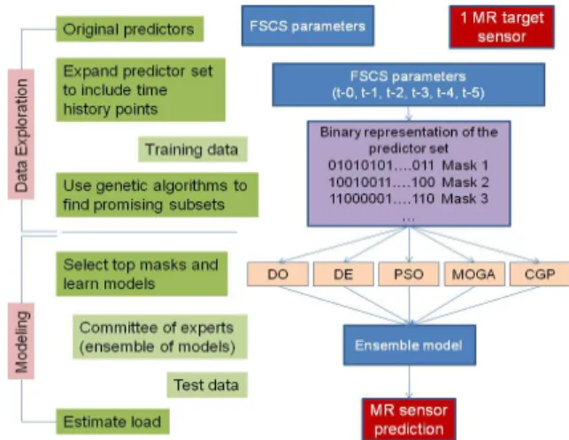
The methodology that was adopted for this work is illus-trated in Figure 1. The application of computational intelli-gence and machine learning techniques to develop these mod-els occurred in two phases: i) data exploration: characterization of the internal structure of the data and assessment of the information content of the predictor variables and its relation to the predicted (dependent) variables; and ii) modeling: build models relating the dependent and the predictor variables.
For the data exploration stage, phase space methods and residual variance analysis (or Gamma test as described in Section III-A) were used to explore the time dependencies within the FSCS parameters and the target sensor variables, identifying how far into the past the events within the system influenced present and future values. This analysis found that 5 time lags were necessary and therefore the predictor set consisted of the 30 FSCS parameters and their 5 time lags for a total of 180 predictors [2]. The Gamma test then steered the evolutionary process used for data exploration. Multi-objective genetic algorithms (MOGA) were used for searching the input space to discover irrelevant and/or noisy information and identify much simpler well-behaved subsets to use as input for modeling. These subsets were found through simultaneous optimization of residual variance, gradient, and the number
Fig. 1. Experimental methodology
of predictor variables. The most promising subsets were then selected and used as a base for model search. The data exploration followed in this work is described in detail in [1]. During the modeling stage, a large number of different computational techniques were implemented to build models relating the target variable to the subset of predictor variables (as identified in the data exploration stage). These techniques included deterministic optimization methods and several evo-lutionary computation techniques.
A. Gamma test (residual variance analysis)
The Gamma test is an algorithm developed by [4], [5], [6] as a tool to aid in the construction of data-driven models of smooth systems. This technique aims to estimate the level of noise (its variance) present in a dataset. Noise is understood as any source of variation in the output (target) variable that cannot be explained by a smooth transformation (model) relating the output with the input (predictor) variables. The fundamental information provided by this estimate is whether it is hopeful or hopeless to find (fit) a smooth model to the data. Since model search is a costly time-consuming data-mining operation, knowing beforehand that the information provided by the input variables is not enough to build a smooth model would be very helpful.
Let us assume that a target variable y is related to the predictor variables x by an expression of the form y = f (x) + r where f is a smooth function and r is a random variable representing noise or unexplained variation. Under some assumptions, the Gamma test produces an estimate of the variance of the residual term using only the available (training) data. A normalized version of the variance, called the vRatio (or Vr), allows the comparison of noise levels
associated to different physical variables expressed in different units across different datasets. Another important magnitude associated with the Gamma test is the so-called gradient, G, which provides a measure of the complexity of the system.
The Gamma test is used in many ways when exploring the data. In the present case, it was used for determining how many time lags were relevant for predicting the future target sensor
values, for finding the appropriate number of neighbours for the computation ofVrandG, and most importantly, for
deter-mining the subset of lagged FSCS variables with the largest prediction potential (therefore the best candidates for building predictive models). In this sense, a comprehensive exploration of the datasets for different target sensors under different flight conditions was made using Gamma test techniques in order to find subsets of the lagged FSCS variables simultaneously with minimal Vr (large prediction power), minimal G (low
complexity) and small in size (cardinality, denoted by #), thus involving a small number of predictor variables. In order to accomplish this task, a multi-objective framework using genetic algorithms was used with <Vr, G, #>as objectives.
B. Construction of the Training and Testing sets
The training/testing sets used for learning the neural net-work parameters and for independent evaluation of their performance should come from the same statistical population in order to properly asses the generalization capability of the network models learnt. Common practices in machine learning work with 50%-90% of the available samples for training and the remaining for testing. In the present case, there was a tremendous amount of data available so in order to keep computing times practical, smaller training sets were constructed. Two methods were used to create the training sets: k-leaders and a biased sampling scheme.
In order to compose a training set with manageable size while still containing a statistically representative sample of the whole dataset, k-means clustering was applied [7]. Ac-cordingly, sets of 2000 clusters were formed using the k-means algorithm with Euclidean distance. Then the data vector closest to its centroid was selected (the so called k-leader). Since every data vector is assigned to a cluster and every cluster has a k-leader as its representative, this sampling procedure ensures that every multivariate vector in the original data is represented in the training sample, and at the same time, that it is a reasonably large set for training purposes.
A second sampling technique to form the training and test-ing sets was explored. For the current problem of estimattest-ing loads in helicopter components, it is important for the models to predict the upper and lower peak values well since these are the values that exert more influence on the lifetime of the helicopter components. In an unbiased sampling scheme, the training and testing distributions should not differ in a statistically significant way. In this work, a biased scheme was used where the probability distribution of the represented classes of values in the training/testing sets was altered to force the learning process to work more with classes of special interest. For example, the abundance of vectors with extreme target values in the training set was made larger than in the whole dataset, so that the networks approximated these values better than lower ones.
IV. NEURALNETWORKTRAININGMETHODS
Training neural networks involves an optimization process, typically focusing on minimizing an error measure. This
operation can be done using a wide variety of approaches ranging from deterministic methods to stochastic, evolutionary computation (EC) and hybrid techniques.
A. Deterministic Optimization
Deterministic optimization (DO) of the root mean squared error (RMSE) or other error measures is the standard practice when training neural networks. Two deterministic optimiza-tion techniques were implemented in this work: conjugate gradient (CJ) and Levernberg-Marquardt (LM). The conjugate gradient method is based on constructing vectors that satisfy orthogonality and conjugacy conditions and do not require the Hessian matrix of second partial derivatives [8]. The Levenberg-Marquardt algorithm works with an approximation of the Hessian matrix (of second derivatives of the error function, in this case, mean-squared) and blends Newton and steepest descent approaches into a single way of computing the optimization parameters (neural network weights) [8]. B. Evolutionary Computation Optimization
1) Particle Swarm Optimization: Particle swarm optimiza-tion (PSO) is a populaoptimiza-tion-based stochastic search process, modeled after the social behavior of bird flocks and similar animal collectives [9], [10], [11]. The algorithm maintains a population of particles, where each particle represents a potential solution to an optimization problem. In the context of PSO, a swarm refers to a number of potential solutions to the optimization problem, where each potential solution is referred to as a particle. Each particlei maintains information concerning its current position and velocity, as well as its best location overall. These elements are modified as the process evolves, and different strategies have been proposed for updating them, which consider a variety of elements like the intrinsic information (history) of the particle, cognitive and socialfactors, the effect of the neighborhood, etc, formalized in different ways. The swarm model used has the form proposed in [12] νidk+1= ω · νk id+ ϕ1· (pkid− x k id) + ϕ2· (pkgd− x k id) xk+1id = xk id+ ν k+1 id ϕi= bi· ri+ di, i = 1, 2 (1)
whereνidk+1 is the velocity component along dimensiond for particle i at iteration k + 1, and xk+1id is its location; b1 and
b2 are positive constants;r1 and r2 are random numbers;d1
andd2 are positive constants to cooperate with b1 andb2 in
order to confine ϕ1 andϕ2 within the interval (0.5, 2); ω is
an inertia weight (see Section V for experimental settings). 2) Differential Evolution: Differential evolution [13], [14] is a kind of evolutionary algorithm working with real-valued vectors. Although relatively less popular than genetic al-gorithms, it has proven to be very effective for complex optimization problems, outperforming other approaches [15], [16]. As in other EC algorithms, it works with populations of individual vectors (real-valued) and evolves them. There are many variants but the general scheme is as follows:
step 0 Initialization: Create a populationP of random vec-tors in ℜn
, and decide upon an objective function f : ℜn → ℜ and a strategy S, involving vector
differentials.
step 1 Choose a target vector from the population ⃗xt∈ P.
step 2 Randomly choose a set of other population vectors V = {⃗x1, ⃗x2, . . .} with a cardinality determined by
strategyS.
step 3 Apply strategy S to the set of vectors V ∪ {⃗xt}
yielding a new vector⃗xt′.
step 4 Add x⃗t or x⃗t′ to the new population according to the value of the objective functionf and the type of problem (minimization or maximization).
step 5 Repeat steps 1-4 to form a new population until termination conditions are satisfied.
There are several variants of DE which can be classified using the notation DE/x/y/z, where x specifies the vector to be mutated, y is the number of vectors used to compute the new one and z denotes the crossover scheme. Let F be a scaling factor,Cr∈ ℜ be a crossover rate, D be the dimension
of the vectors, P be the current population, Np = card(P)
be the population size, ⃗vi, i ∈ [1, Np] be the vectors of P,
⃗bP ∈ P be the population’s best vector w.r.t. the objective
function f and r, r0, r1, r2, r3, r4, r5 be random numbers in
(0, 1) obtained with a uniform random generator function rnd() (the vector elements are ⃗vij, where j ∈ [0, D)). Then
the transformation of each vector⃗vi∈ P is performed by the
following steps:
step 1 Initialization:j = (r · D), L = 0 step 2 while(L < D)
step 3 if ((rnd() < Cr)||L == (D − 1))
/* create a new trial vector. For example, as: */ ⃗tij = ⃗bPj+ F · (⃗vr1j+ ⃗vr2j− ⃗vr3j− ⃗vr4j) step 4 j = (j + 1) mod D
step 5 L = L + 1 step 6 goto 2 step 7 stop
Many particular strategies have been proposed that differ in the way the trial vector is constructed (step 3 above). In this paper theDE/rand/1/exp strategy was used as it has worked well for most problems (see Section V for experimental settings).
3) Multi-Objective Genetic Algorithms: An enhancement to the traditional evolutionary algorithm is to allow an individual to have more than one measure of fitness within a popula-tion. This modification may be applied through the use of a weighted sum of more than one fitness value [17]. MOGA, however, offers another possible way for enabling such an enhancement. In the latter case, the problem arises for the evolutionary algorithm to select individuals for inclusion in the next population, because a set of individuals contained in one population exhibits a Pareto Front [18] of best current individuals, rather than a single best individual. Most [17] multi-objective algorithms use the concept of dominance. A solution↼
x(1) is said to dominate [17] a solution
↼ x(2)for a set of m objective functions < f1( ↼ x), f2( ↼ x), ..., fm( ↼ x) > if 1) ↼
x(1) is not worse than
↼
x(2) over all objectives.
For example, f3( ↼ x(1)) ≤ f3( ↼ x(2)) if f3( ↼ x) is a mini-mization objective. 2) ↼
x(1) is strictly better than
↼
x(2) in at least one
objec-tive. For example, f6(↼x(1)) > f6(↼x(2)) if f6(↼x) is a
maximization objective.
One particular algorithm for MOGA is the elitist non-dominated sorting genetic algorithm (NSGA-II) [19], [20], [21], [17]. It has the features that it i) uses elitism, ii) uses an explicit diversity preserving mechanism, and iii) emphasizes the non-dominated solutions. The procedure is as follows: i) Create the child population using the usual genetic algorithm operations. ii) Combine parent and child populations into a merged population. iii) Sort the merged population according to the non-domination principle. iv) Identify a set of fronts in the merged population (Fi, i = 1, 2, ...). v) Add all complete
fronts Fi, for i = 1, 2, ..., k − 1 to the next population. vi) If
there is a front,Fk, that does not completely fit into the next
population, select individuals that are maximally separated from each other from the front Fk according to a crowding
distance operator. vii) The next population has now been constructed so continue with the genetic algorithm operations. 4) Cartesian Genetic Programming: Cartesian genetic pro-gramming (CGP) is a kind of genetic propro-gramming (GP) first formulated in [22], [23], motivated by learning boolean functions, novel design of digital circuits and their automatic evolution. It was formulated as a new kind of generic program-ming in [24]. In CGP, programs are represented as a list of integers that encode the connections and functions correspond-ing to directed graphs where the genotype is a fixed-length representation and each node represents a particular function from a function set which is encoded by a number of genes. The phenotypes are of variable length according to the number of unexpressed genes. A gene encodes the function that the node represents, and the remaining genes encode where in the graph the node obtains its inputs from. The nodes take their inputs in a feed-forward manner from either the output of nodes in a previous column or from a program input (terminal). A Cartesian program (CP) denoted P is defined as a set {G, ni, no, nn, F, nf, nr, nc, l} where G represents the
geno-type and is itself a set of integers representing the indexedni
program inputs, thenn node input connections and functions,
and thenoprogram output connections. The setF represents
the nf functions of the nodes. The number of nodes in a
row and column are given by nr, nc respectively. Finally
the program inter-connectivity is defined by the levels back parameter l, which determines how many previous columns of cells may have their outputs connected to a node in the current column [24]. The CGP’s genotype-phenotype mapping does not require all of the nodes to be connected to each other. The phenotypes can have a length from zero to the maximum number of nodes encoded in the genotype and there may be areas of the genotype that are present, but inactive, thus having no influence (genetic operators could activate/deactivate genes).
C. Hybrid and Memetic Approaches
A common issue of deterministic (gradient-based) tech-niques is the local entrapment problem and it can be mitigated by combining local and global search techniques. In this case, deterministic optimization with evolutionary computa-tion methods, both presented above. Several hybridizacomputa-tion approaches are possible: i) coarse and refinement stages: Use a global search technique and upon completion, go to a next step of using a subset of the solutions (proper or not) as initial approximations for local search procedures (e.g. deterministic optimization methods). The final solutions will be those found after this second step, ii) memetic: Embed the local search within the global search procedure. In this case the evaluation of the individual constructed by the global search procedure is made by a local search algorithm. For example, within an evolutionary computation procedure, the evaluation of the fitness of an individual is the result of a deterministic optimization procedure using as initial approximation the individual provided by the evolutionary algorithm. Then, the EC-individual is redefined accordingly and returned to the evolutionary procedure for the application of the evolutionary operators and the continuation of the evolutionary procedure. In this paper both hybridization procedures were used. The results of their application to the helicopter load estimation problem are discussed in Section VI.
V. EXPERIMENTALSETTINGS
A. Data exploration - MOGA settings
During the data exploration by the MOGAs as guided by the Gamma test, 150 runs were made for each of the flight condi-tions and training schemes. The experimental settings included allowing elitism, using a number of crossover probabilities (0.3, 0.5, 0.6, 0.8, 0.9) and mutation probabilities (0.01, 0.025, 0.05), and 10 random seeds. Each experiment consisted of 1000 objects that were allowed to evolve over 300 generations producing 1000 solutions. Therefore for each case, a total of 15000 subsets (or masks) were produced.
B. Neural Network Configurations
In this study, the models were all feed-forward neural networks that were trained using one of13 different methods: CJ, LM, pure PSO, PSO with CJ, PSO with LM, memetic CJ-PSO, memetic LM-CJ-PSO, pure DE, DE with LM, DE with CJ, memetic CJ-DE, memetic LM-DE, and MOGA. A number of network configurations were attempted including those with one or two hidden layers with1 to 12 neurons in each hidden layer. The output layer used a linear transfer function, while the hidden layers used a tanh transfer function. Each trial was repeated up to3 times initialized with a different random seed. In total there were 2088 runs for each case (flight condition/sampling scheme) with an imposed time limit (3 hours) and maximum number of iterations allowed (10000).
The network configurations and settings were selected based on either recommended values from literature, previous settings that obtained good results, or simply to cover the allowable parameter range. The settings for PSO and DE are
TABLE I
EXPERIMENTALSETTINGS FORPSOANDDE PSO settings DE settings Parameter Value Parameter Value # of particles 10 Population Size 20 b1,b2 1.5, 1.5 F 0.5 r1, r2 rnd[0, 1],rnd[0, 1] CR 0.8 d1, d2 0.5, 0.5 ri rnd([0,1]) range of x0 i [−3, 3] range of x 0 i [−3, 3] range of v0 i [1, 5] Strategy DE/rand/1/exp described in Table I. The MOGA optimized 2 objectives (MSE and correlation), had a population size of 100, used a crossover probability of0.9 and mutation probability of 0.5, and allowed for 1000 generations.
CGP was used with population sizes {3, 5} individuals, mutation rates in {0.05, 0.1, 0.25, 0.5, 0.7, 0.8}, and five dif-ferent seeds for generating initial populations. The number of rows and columns used were {1}, {100, 150, 300, 400} respectively. In each run the evolution was allowed to go up to 500000 generations. Three error functions were used: i) mean absolute error (MAE), ii) mean squared error (MSE), and iii) an asymmetric fuzzy-based error function E(x, T ) given by(1/S(x, T ))−1. S(x, T ) is a membership function of predicted valuesx with respect to the class defined by a target value T . For T ≥ 0, it is defined piecewise as S(x, T ) = 1 if |x| − |T | ≤ ϵ, S(x, T ) = (1/(1 + (αu|x − T |))) if x < T
and S(x, T ) = (1/(1 + (αo|x − T |))) if x ≥ (T + ϵ). For
T < 0, S(x, T ) = S(x, −T ). The parameters of the S function (ϵ, αu, αo) were set to0.15, 10 and 1 respectively in order to
stimulate slight to moderate overprediction (that is, conser-vative estimates, provided that the target variable represents a helicopter load). This asymmetric error function contrasts the MAE and MSE error measures which are symmetric and therefore do not differentiate under and overprediction. C. Biased Training and Testing Set Construction
In each flight recording, the FSCS and target data tuples were partitioned into a training and testing set. The training set was constructed such that it contained a higher proportion of the upper and lower values in the target signal than in the original recording. The threshold defining these regions, or classes, was set as a function of the mean and standard devi-ation of the target signal: the data points exceeding the mean plus 1 standard deviation belonged to the ‘high’ class, those below the mean minus 1 standard deviation fell in the ‘low’ class, and the remaining data were assigned to the ‘medium’ class. The distribution between the high, medium, and low classes was arbitrarily set as 0.4, 0.2 and 0.4 respectively.
VI. RESULTS
The original predictor set of 30 FSCS parameters was expanded to 180 to include their time history data (as dis-cussed in Section III). Using MOGA and the Gamma test, reduced subsets of predictor variables were found during the data exploration phase and the most promising subsets were used to build models estimating the main rotor normal
bending (MRBNX) for three flight conditions. The models were all feed-forward neural networks that used the various computational intelligence techniques for building the models. Ensembles of the top models were then formed for each case. A. Full mask vs reduced mask results
Searching for subsets of input variables with predictor potential, the exploration using MOGA in combination with the Gamma test generated 15000 solutions for each case. The task of searching the input space for suitable subsets was no simple task since with 180 predictor variables, there were 2180 − 1 subsets to consider as input variables for
modeling. This huge number, however, only includes the potential combinations of variables; the number of potential models that could be formed from the different combinations of variables is infinite. Therefore the 15000 subsets that were generated by the MOGA represent only a tiny fraction of that space. For all the cases examined in this work, the MOGA was able to find a large number of solutions with a greatly reduced set of predictor variables, indicating that the original input set contained a large amount of irrelevant and noisy data. The MOGA masks provided two important pieces of information for the modeling stage: i) a reduced input parameter set emphasizing parameters with predictive potential, and ii) a target error threshold (vRatio) to aim for during training.
A comparison of the estimates for the target output using the full mask and the most promising mask found by the MOGA and Gamma test shows the effectiveness of this approach to sort through the information contained in the FSCS parameters. Table II gives the results (root mean squared error (RMSE) and correlation (corr)) for MRNBX level flight of ensembles using models trained with PSO and DE. These ensembles were formed from the top models using either pure EC, coarse-refinement DO-EC, or memetic DO-EC.
TABLE II
COMPARISON OF FULL MASK AND REDUCED MASK RESULTS FOR
MRNBXLEVEL FLIGHT USING K-LEADER SAMPLING
MRNBX Training Testing level flight RMSE corr RMSE corr Full mask PSO 0.429 0.886 0.621 0.786 180 parameters DE 0.291 0.962 0.615 0.796 MOGA mask PSO 0.439 0.883 0.670 0.746 26 parameters DE 0.328 0.940 0.611 0.797
For the case of the full mask, the EC techniques were searching an enormous space with dimensionality of2180− 1.
The fact that the EC techniques were able to generate rea-sonably accurate and correlated models for MRNBX given that difficult task is quite remarkable. Although the training performance of the DE ensemble as compared to the PSO ensemble was much better on the training set, the difference between the two EC techniques in testing was very small.
For the case of the reduced mask, it had only 26 variables compared to the 180 of the full mask corresponding to a significant 85 % reduction in size. The models generated using this reduced mask yielded predictions with very similar
if not better performance than those obtained with the full mask. Even though the full mask contained the same variables as the most promising mask, it is evident that having to accommodate all of the variables, including those the GA deemed superfluous and noisy, detracted from its performance. The use of MOGA and the Gamma test to identify and exclude noisy and irrelevant parameters then was successful. This result is encouraging, as it indicates that simpler models could be constructed using the MOGA masks without sacrificing performance. This approach using MOGA and Gamma test to identify subsets with predictive power was followed for all the cases examined in this work and as will be discussed in Section VI-C, models with good performance were found for all of these cases demonstrating the effectiveness of the approach.
B. Behavior of pure vs hybrid EC approaches
Table III shows the results of the models for the MRNBX steady turn flight condition using biased training. The table compares the use of DO alone, the EC techniques alone, and then in the two hybrid combinations (coarse-refinement and memetic). Using any of the EC techniques alone generated
TABLE III
MRNBXSTEADY TURN BIASED TRAINING
Training Testing Learning Method RMSE corr RMSE corr Pure DO 0.347 0.942 0.620 0.528 Pure PSO 0.823 0.609 0.576 0.347 PSO-DO coarse/ref 0.399 0.924 0.585 0.555 PSO-DO memetic 0.533 0.857 0.590 0.531 Pure DE 0.770 0.676 0.554 0.441 DE-DO coarse/ref 0.234 0.976 0.596 0.560 DE-DO memetic 0.181 0.985 0.598 0.566
fair predictions for MRNBX. However, the addition of DO, specifically the Levenberg-Marquardt learning method, greatly improved the training predictions (RMSE and correlation). In testing, while improvements in the RMSE were small, the correlation was significantly improved in the hybrid versions. It should be noted that the models were trained to optimize the MSE and not correlation. For PSO, the best hybrid was the coarse-refinement approach using LM. In contrast, the best performance for DE was as a memetic DE-LM approach.
Figure 2 shows the remarkable change in the quality of the prediction for PSO from a pure to a hybrid format. It is worth noting that while the testing performance as listed in Table III shows similar RMSE values for these two cases (pure PSO and coarse-refinement PSO-DO), the plots in Figure 2 show that the coarse-refinement PSO-DO model yielded a much closer prediction at the peak values and overall better coverage of the target signal. The difference between the two plots is much more noticeable than one would expect given the small difference in performance values. For this flight condition, the prediction by DO alone was quite strong. However, the hybrid predictions were able to provide some improvement to the pure DO prediction in testing in terms of RMSE and
Fig. 2. Testing predictions for MRNBX steady turn using biased sampling. The upper plot shows the pure PSO prediction. The lower plot shows the significant improvement obtained using coarse-refinement PSO-LM. The dashed vertical lines indicate the boundary between different flight recordings.
correlation. These trends were consistent for all the MRNBX flight conditions.
C. Comparison of EC techniques
Table IV lists the results for all the models of MRNBX for the three flight conditions and training schemes. As dis-cussed previously, the PSO and DE hybrid models generated reasonably accurate and correlated predictions with similar performance. The DE hybrid ensembles had impressive results in training that were much better than PSO or DO results. However in testing, this difference was much smaller and overall the performance was similar for the PSO, DE, and DO techniques. There was some underprediction for all methods in the three flight conditions, particularly for the k-leaders train-ing scheme, but the frequency and degree of underprediction was much reduced as compared to previous results [1].
While the results achieved by the MOGA model according to the RMSE and correlation were largely outperformed by the other techniques (refer to Table IV), some interesting observations arose when the time-series predictions were in-spected. For all the flight conditions and training schemes, even when all the other modeling techniques (DE, PSO, DO) were underpredicting the target signal, the MOGA models consistently overpredicted the target. While the overprediction was sometimes by a wide margin (sometimes 2 or 3 times the target value causing large RMSE values), rarely did the MOGA model underpredict the target. From the point of view of helicopter load prediction, this tendency to overpredict rather than underpredict is preferable to ensure conservative estimates for component life. This is not to say that an overprediction by 2 or 3 times is desirable but perhaps further exploration and finetuning of the MOGA parameters might temper the margins. For future studies it may be worth evaluat-ing the damage fraction from the predicted signal generated by
TABLE IV
ENSEMBLE RESULTSMRNBXFOR LEVEL FLIGHT,ROLLING PULLOUT,
AND STEADY TURN USING K-LEADERS OR BIASED SAMPLING
Flight Sampling Learning Training Testing condition scheme method RMSE corr RMSE corr Level k-leaders DO 0.371 0.918 0.655 0.758 flight PSO 0.439 0.883 0.670 0.746 DE 0.328 0.940 0.611 0.797 MOGA 1.800 0.665 1.825 0.611 Level biased DO 0.266 0.965 0.444 0.800 flight PSO 0.343 0.941 0.460 0.766 DE 0.231 0.974 0.407 0.829 MOGA 1.007 0.705 1.138 0.502 Rolling k-leaders DO 0.702 0.700 0.938 0.434 pullout PSO 0.629 0.784 0.839 0.550 DE 0.571 0.833 0.823 0.573 MOGA 1.501 0.488 1.535 0.441 Rolling biased DO 0.479 0.887 0.608 0.461 pullout PSO 0.554 0.840 0.633 0.434 DE 0.410 0.916 0.706 0.420 MOGA / / / / Steady k-leaders DO 0.494 0.869 0.793 0.632 turn PSO 0.524 0.857 0.764 0.659 DE 0.432 0.912 0.700 0.727 MOGA 2.069 0.529 2.062 0.462 Steady biased DO 0.347 0.942 0.620 0.528 turn PSO 0.403 0.920 0.609 0.547 DE 0.179 0.986 0.593 0.565 MOGA 1.448 0.409 1.396 0.307
each network and comparing it to that of the observed signal, which would give a better indication than RMSE/correlation of which network was better suited for this problem.
Overall, the level flight condition was the simplest manoeu-vre to model and was well predicted by all methods including the peak values. Prediction of the steady turn manoeuvre was a more challenging task, however, the hybrid EC-DO models were able to generate impressive predictions for the target signal (as seen in Figure 2). The rolling pullout manoeuvre was a more difficult flight condition to predict and not surprisingly the performance of the models was not as strong in terms of RMSE and correlation. However, inspecting the time signal predictions for this manoeuver show that the peak values were captured quite well in many cases, particularly at the extreme values which are the areas most critical for helicopter structural integrity. The fact that reasonable results could be found for this difficult manoeuvre is very encouraging.
Although a number of EC techniques were used, this study was by no means an exhaustive exploration of the EC potential in this problem - only a simple PSO model was used, only one of many DE strategies was implemented, a strict limit on the number of generations was set, and there was no variation of the EC controlling parameters (fixed particle velocity ranges, coefficients, etc). There are still other EC techniques worth considering such as evolution strategies and other variants of DE and GP, among others.
D. Effect of different error functions
A cursory exploration of the effect of using different error functions was carried out using Cartesian GP. These error functions included mean absolute error (MAE), mean squared
error (MSE), and the asymmetric error function defined in Sec-tion V-B. All the parameter settings were identical except for the error function, therefore any differences in the predictions can be attributed to the change in the error function. Figure 3 shows the predictions for MRNBX level flight using the biased training scheme from CGP using MSE and the asymmetric error function. Using MSE as the error function (upper plot), it can be seen that the predicted signal was quite accurate, however, there were many areas that were underpredicted. In contrast, the use of the asymmetric error function (lower plot) resulted in consistent overprediction of the target signal at both the upper and lower boundaries, even though occasionally the margin of overprediction was quite large. As mentioned previously, this tendency to overpredict (vs. underpredict) is preferable to ensure conservative helicopter load estimates. While this exploration was very brief, the results are very promising and further investigation into the use of alternative asymmetric error functions should be pursued as a way to encourage overprediction of the target signal (and discourage underprediction).
Fig. 3. CGP predictions for MRNBX level flight using different error functions. The upper plot shows the CGP prediction using MSE, while the lower plot shows the CGP prediction using the asymmetric error function.
VII. CONCLUSIONS
This work expanded the use of computational intelligence techniques and sampling methods to predict several main rotor loads on the Black Hawk helicopter through three flight conditions of varying complexity. EC techniques played an important role in both the exploratory and modeling phase of the investigation. The use of MOGA optimizing several Gamma test measures allowed the identification of smaller subsets of relevant FSCS parameters with predictive value, as well as irrelevant and noisy variables for all of the flight conditions studied. When used as inputs to neural networks trained with EC, and particularly with hybrids of EC and DO techniques, well behaved ensemble models were found in terms of prediction errors and correlation measures for both
the training and testing sets for all flight conditions considered. Future work should incorporate other relevant EC techniques, a more comprehensive study of those used and other error measures providing more control of the over/under prediction model behavior, and calculating fatigue damage based on the predicted loads to better evaluate the quality of the predictions.
REFERENCES
[1] J. J. Valdes, C. Cheung, and W. Wang, “Evolutionary computation methods for helicopter loads estimation,” in Proc. IEEE Congr. on Evol.
Computation, New Orleans, LA, USA, June 2011.
[2] ——, “Computational intelligence methods for helicopter loads estima-tion,” in Proc. Int. J. Conf. on Neural Networks, San Jose, CA, USA, Aug 2011, pp. 1864–1871.
[3] Georgia Tech Research Institute, “Joint USAF-ADF S-70A-9 flight test program, summary report,” Georgia Tech Research Institute, Tech. Rep. A-6186, 2001.
[4] A. Jones, D. Evans, S. Margetts, and P. Durrant, “The gamma test,”
Heuristic and Optimization for Knowledge Discovery, 2002.
[5] A. Stef´ansson, N. Kon˘car, and A. Jones, “A note on the gamma test,”
Neural Computing and Applications, vol. 5, pp. 131–133, 1997. [6] D. Evans and A. Jones, “A proof of the gamma test.” Proc. Roy. Soc.
Lond. A, vol. 458, pp. 1–41, 2002.
[7] M. Anderberg, Cluster Analysis for Applications. London UK: John Wiley & Sons, 1973.
[8] W. Pres, B. Flannery, S. Teukolsky, and W. Vetterling, Numeric Recipes
in C. Cambridge University Press, 1992.
[9] J. Kennedy and R. C. Eberhart, “Particle swarm optimization,” in Proc.
IEEE Int Joint Conf on Neural Networks, vol. 4, 1995, pp. 1942–1948. [10] J. Kennedy, R. C. Eberhart, and Y. Shi, Swarm Intelligence. Morgan
Kaufmann, 2002.
[11] M. Clerc, Particle Swarm Optimization. ISTE Ltd, 2006.
[12] Y. Zheng, L. Ma, L. Zhang, and J. Qian, “Study of particle swarm optimizer with an increasing inertia weight,” in Proc. World Congr. on
Evol. Computation, Canberra, Australia, Dec 2003, pp. 221–226. [13] R. Storn and K. Price, “Differential evolution-a simple and efficient
adaptive scheme for global optimization over continuous spaces.” ICSI, Tech. Rep. tr-09012, 1995.
[14] K. V. Price, R. M. Storn, and J. A. Lampinen, Differential Evolution.
A Practical Approach to Global Optimization., ser. Natural Computing Series. Springer Verlag, 2005.
[15] S. Kukkonen and J. Lampinen, “An empirical study of control parame-ters for generalized differential evolution.” Kanpur Genetic Algorithms Laboratory (KanGAL), Tech. Rep. 2005014, 2005.
[16] R. G¨amperle, S. D. M¨uller, and P. Koumoutsakos, “A parameter study for differential evolution.” [Online]. Available: citeseer.ist.psu.edu/526865.html
[17] E. Burke and G. Kendall, Search Methodologies: Introductory Tutorials
in Optimization and Decision Support Techniques. New York: Springer Science and Business Media, 2005.
[18] V. Pareto, Cours D’Economie Politique. volume I and II. Lausanne: F. Rouge, 1896.
[19] K. Deb, A. Pratap, S. Agarwal, and T. Meyarivan, “A fast and elitist multi-objective genetic algorithm - NSGA-II.” Kanpur Genetic Algo-rithms Laboratory, Tech. Rep. 2000001, 2000.
[20] K. Deb, S. Agarwal, A. Pratap, and T. Meyarivan, “A fast elitist non-dominated sorting genetic algorithm for multi-objective optimization: NSGA-II,” in Proc. Parallel Problem Solving from Nature VI Conf., Paris, 16-20 September 2000, pp. 849–858.
[21] K. Deb, A. Pratap, S. Agarwal, and T. Meyarivan, “A fast and elitist multiobjective genetic algorithm: NSGA-II,” IEEE Trans. on Evol.
Comput., vol. 6 (2), pp. 182–197, 2002.
[22] J. F. Miller, “An empirical study of the efficiency of learning boolean functions using a cartesian genetic programming approach,” in Proc.
1999 Genetic and Evol. Computation Conf. (GECCO 99), Orlando, Florida, USA, 1999, pp. 1135–1142.
[23] J. Miller, D. Job, and V. Vassilev, “Principles in the evolutionary design of digital circuitspart I.” Genet. Program. Evol. Machines, vol. 1, no. 1, pp. 8–35, 2000.
[24] J. F. Miller and P. Thomson, “Cartesian genetic programming,” in LNCS, R. Poli, W. Banzhaf, and et al., Eds., vol. 1802. Springer Verlag, 2000, pp. 121–132.