A dimensionality reduction process to forecast events through stochastic models

HAL Id: hal-01247905

https://hal.inria.fr/hal-01247905

Submitted on 23 Dec 2015

HAL is a multi-disciplinary open access

archive for the deposit and dissemination of

sci-entific research documents, whether they are

pub-lished or not. The documents may come from

teaching and research institutions in France or

abroad, or from public or private research centers.

L’archive ouverte pluridisciplinaire HAL, est

destinée au dépôt et à la diffusion de documents

scientifiques de niveau recherche, publiés ou non,

émanant des établissements d’enseignement et de

recherche français ou étrangers, des laboratoires

publics ou privés.

A dimensionality reduction process to forecast events

through stochastic models

Joaquim Assunção, Paulo Fernandes, Lucelene Lopes, Silvio Normey

To cite this version:

Joaquim Assunção, Paulo Fernandes, Lucelene Lopes, Silvio Normey. A dimensionality reduction

pro-cess to forecast events through stochastic models. International Conference on Software Engineering

and Knowledge Engineering, Jul 2015, Pittsburgh, United States. �hal-01247905�

A DIMENSIONALITY REDUCTION PROCESS TO FORECAST EVENTS

THROUGH STOCHASTIC MODELS

Joaquim Assunção, Paulo Fernandes, Lucelene Lopes, Silvio Normey

PUCRS University – Computer Science Department – Porto Alegre, Brazil

{joaquim.assuncao, paulo.fernandes, lucelene.lopes, silvio.gomez}@pucrs.br

Abstract

This paper describes a dimensionality reduction process to forecast time series events using stochastic models. As well as the KDD process defines a sequence of common steps to achieve useful in-formation through data mining techniques, we propose a sequence of steps in order to estimate the probability of future events through stochastic modeling. Our process focus on reduce the dimension-ality of data, thus reducing the effect of the common problems in-volved in stochastic modeling, such as the state space explosion and the large modeling efforts to create such models.

1 Introduction

Stochastic modeling can be a natural option to predict system behavior. This system can be a process that represents basic situations or even complex nature events. Either way, a good model can deliver interesting probabilities about system events for its past, or even its future.

However, modeling is a non trivial task that requires a specialist on the domain that have a good knowledge about the scenario to be modeled. Other problem frequently faced, with stochastic models, is the state space explosion that causes a limit of states, thus, a limit of data to be modeled.

The amount of data in the world, in our lives, seems to go on and on increasing [32], and as the volumes of data increase, it increases the difficulty of handling these data. One of the problems most frequently faced is the difficult to detect information among such large amounts of data. These informations are lost because it is hard for a human being to see the patterns and relations among such abundant data.

To cope with this problem, specialized data mining algorithms retrieve information that are practically invisible to our perception. Although the information is revealed, it is not yet knowledge, since knowledge must be obtained by rationally processing the extracted information. Aiming to formalize the steps commonly used to reach the knowledge through data mining, there are some well defined processes in the literature, as for example the knowledge discovery in databases (KDD) described by Han et al. [17]. Although this process is well consolidated and often used as a guide for knowledge discovery, instead of describing the path to discover knowledge, it seems to have been created to cover the steps that usually come before and after data mining.

In the context of our paper we focus on a specific case of KDD, which is the forecast of future events in time series databases. Therefore, we propose the use of stochastic modeling techniques as steps of the proposed process, information about events is a common trade in stochastic models. Specifically, we simulate and analyze a formal state-based model of the system in order to retrieve probabilities for future events (and states) of the targeted system.

In a rough comparison. as well as KDD shows a set of steps commonly used to prepare data for data mining, here we describe a process that shows useful steps to prepare data for stochastic modeling. These steps aim to decrease the time spent to develop models, coping with state space problem and reducing the chance of human mistakes while manually developing complex models.

This paper is organized as follows: the next sections describe this paper background: Time series and Stochas-tic modeling formalisms; The fourth section puts this work in perspective with pre-existent techniques; The fifth section describes the proposed process; Section 6 illustrates the pro-posed process with some numerical result obtained applying it to pre-existent datasets; Finally, the conclusion summa-rizes our contribution and suggests future works.

2 Time Series

A popular method to represent and analyze data is time series (TS) [8, 21, 31]. Given the ease of use, modify, compare and analyze data; TS became very popular in many fields of sciences such as statistics, economy, biology, geography, seismology, engineering, communication, machine learning, etc. A TS is characterized as a collection of data spread in time. Formally, a TS S can be defined as follows:

S= [(p1,t1), (p2,t2), ..., (pk,tk), ...(pn,tn)]

(2.1)

where (t1< t2< ... < tk< ... < tn)

In this representation, piis the data corresponding to the

i-th observation, and tiis the time when piwas observed. In

such way, a TS can be visualized in two axis, one with the data representing pi, and other with the time passage from

t1to to tn. Despite of that, since the data associated to each

observation can be be related to a complex information, TS are essentially high dimensional data [17]. In fact, TS can be employed to describe very complex structures like fossil shapes, molecules, geological materials, etc. [34, 18].

In order to enhance the ease of storage, to facilitate human analysis, and to be flexible to many domains, TS had became a global trending for representation of data. Consequently, the constant use of TS in different areas and the growth of machine learning, brought researchers to new challenges related to TS.

We can highlight such challenges according to the main goals of TS analysis: modeling and forecasting [17]. In modeling, researchers try to improve efficiency by reducing the impact of the dimensionality factor and by improving measurements techniques. In forecasting, researchers try to predict future situations, e.g., weather forecast, traffic behavior, etc.

One of the big problems related to TS is how to im-prove modeling efficiency being TS generally a data stream-ing [31]. Aimstream-ing to solve this problem, in the last decade, many methods to represent TS have been created [25, 8, 20].

3 Stochastic Modeling

Stochastic modeling is the art of representing the behavior of a system by describing its states and transitions. One of the most common among such formalisms are the Markov chains. Given an initial state, even a simple discrete-time Markov chain can be used to forecast future states by achieving probabilities for each possible state for the next n steps [29]. These steps are given by the Chapman-Kolmogorov equation. Being P a probability matrix:

P_{i j}(m)=

_∑

all k

P_ik(l)P_{k j}(m−l) f or0 < 1 < m

(3.2)

Being a classic formalism, Markov chains are easy to handle and use to perform quantitative analysis. Unfortu-nately large volumes of data tend to generate huge models that are hard to handle using an ordinary Markov chain (state space explosion). In such cases, the use of a structured for-malism as Stochastic Automata Networks (SAN) [24, 7] may reduce this problem impact.

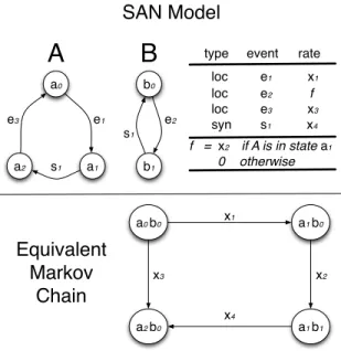
SAN is a formalism that describes a complete system as a collection of subsystems that interact with each other in a Markovian behavior. The main advantage of SAN is that we can represent very large and complex system in a human understandable model that has an equivalent Markov chain model. Figure 1 exemplifies a SAN model with two automata and its equivalent Markov chain.

SAN formalism uses synchronized events and func-tional rates to build the system. Once a model is ready, with few automata it can be equivalent to a giant Markov chain. In

a0 a1 a2 b1 b0 e1 e3 e2 s1 s1 a0 b0 a1 b0 a2 b0

type event rate

loc e1

Equivalent

Markov

Chain

A

B

SAN Model

Figure 1: SAN model example with 2 automata and its equivalent Markov Chain.

addition, the tensor format of SAN makes possible the use of specialized algorithms [15, 10, 11] which are more efficient than those used for solving large Markov chains [10, 11]. A complete SAN model is represented by a SAN code that can be executed [6] to generate a set of probabilities, including those which may be generated in a Markov chain.

Recently we successfully created a SAN model to rep-resent and predict classes in geological events [1]; a different approach that returns results much similar to a data mining classification. Due to the processes of analysis and data col-lection, this model took much time to be created. However, even high dimensional data can be transformed into TS, and then, into a string that can be transformed both into a SAN model or into a Markov chain.

4 Dimensionality Reduction and Forecast

Both research areas, TS and stochastic modeling, have an in-teresting thing in common; they both have many applications that are useful for knowledge discovery. The use of TS for data representation and forecasting is presented in a myriad of works [9, 26, 23, 22, 4]. Despite such abundant material, is also frequent to found the use of Markovian models to predict states in complex scenarios [13, 35, 28, 5, 16, 1, 14]. In this work, we use these both techniques trying to profit from the knowledge on TS modeling and stochastic predic-tion through Markovian models.

Using stochastic modeling techniques, we can retrieve accurate probabilities about a given system or event. How-ever, the “state space explosion” makes it hard to scale models to real application size problems [30, 29]. In TS

there is a similar phenomenon, the well-known “curse of di-mensionality”, which is the subject of many works in the area [25, 8, 21].

Actually, these two problems are different views of a same phenomenon, since the background limitation is the fact that it is easy to describe a large number of points of view (several dimensions), but the reality that needs to be handled is the Cartesian product of the data from all this points of view, i.e., we model focusing on the parts, but the model must be handle as a whole. Among the approaches to tackle this problem, we are interested in this paper in dimensionality reduction [21] and structured modeling formalisms [7].

Several techniques have been developed to represent TS in order to reduce the difficulty of processing high dimensional data. Here, we are interested in techniques that have two characteristic: 1) the representation must be symbolic; 2) the representation must be flexible in length. Among this techniques, for experiment purposes, we use Symbolic Aggregate approXimation (SAX) [21].

SAX is a solution to reduce the dimensionality of a TS both in length (it reduces the number n of observations) and in data space (it aggregates the values of pi). Also,

it generates symbolic data that can be used to generate stochastic models on an automated way. The next section presents the process, and the basic phases to obtain the stochastic model, and then, the data forecasting through its transient and steady states analysis.

5 Proposed Process

Instead of work directly in mathematical models to slight improve some stochastic formalism, we focus on a process that reduces the data dimensionality before these data goes into the model. Instead of use a limited set of algorithms to forecasting in TS, we focus on adapt these data to work with advanced stochastic algorithms.

In order to achieve it, we carefully select the most use-ful techniques to represent and reduce the dimensionality of a given dataset, as well as, powerful methods that allow us to perform quantitative analysis under the generated data. Thus, this process aims to achieve a set of useful probabili-ties directly from a dataset using the minimum human effort and minimizing the effects of “state space explosion".

Figure 2 shows a simplified flow diagram of the pro-posed process. Each picture represented at the bottom part of this figure is a set of data; and each term written at the top part of this figure is a task of the process. Next, we describe each step of the process, which is basically composed by a task and its resultant data .

5.1 Data Selection Given a database, the first step begins with Data Selection. The Data Selection described here is very similar to the data mining Data Selection step; the data

DATABASE DATA SELECTION TIME SERIES DATASET TS REPRESENTATION METHODS CODER _SOLUTIONSM SYMBOLIC DATA STOCHASTIC MODEL TRANSIENT/STEADY STATE PROBABILITIES

Figure 2: Process Phases

must be analyzed aiming to retrieve the desired TS. After this step, a set of TS is achieved.

5.2 TS Representation This step performs the dimen-sionality reduction of the dataset. One by one, the TS goes to SAX which performs a dimensionality reduction using Piecewise Aggregate Approximation [8]. Then, SAX gen-erates the symbolic data.

5.3 Coder In big data, coding is the process of tagging terms using an identifier that is assigned to every synony-mous term in the data [3]. This step has a similar objec-tive; although, instead of grouping terms, symbolic data are grouped into states. Thus, this step is the connection be-tween TS output and the solution of the SM. In other words, Coder is the step responsible to get the symbolic data gen-erated by TS representation and transform it into a SM. As seen in the Figure 3, the symbolic data is a collection of N symbols that represents N levels of a given TS; thus, repre-sented by: S = [a, b, c, d, ...Ω] the symbolic data generated (D) can be formalized as: Di= {s ∈ S}.

Figure 3: Classes and symbolic data generated for Coffee dataset, an example of TS dataset.

Once we have the symbolic data, it is possible to auto-matically create the SMs. Basically it is performed by get-ting the frequencies of changes for each class in a symbolic data.

Given three hypothetically TS, Q, S and T and its repre-senting symbolic data w(Q), w(S) and w(T ), each one com-posed by classes from a to j. The coder calculates the fre-quency of changes for each possible combination, e.g.:

a→ b, a → c, ... , a → j b→ a, b → c, ... , b → j ... , ... , ... , ... j→ a, j → b, ... , j → j

Each frequency is turned into a percentage value that is used as a transition rate for the automata. Also, each set of symbolic data turns in one automaton. In this scenario, we will have a SAN composed by three automata created from w(Q), w(S), w(T). Having each one 10 states, e.g., a, b, . . . , j, our SAN model will be limited to 1000 reachable states, which is almost instantaneously to solve with current SAN algorithms.

5.4 Stochastic model solution In this step, the code gen-erated is used to create and solve a stochastic model. These stochastic models can be either, Markov chains, SAN or any other Markovian formalism. We develop a tool to make au-tomatically create Markovian models from a symbolic data; furthermore, there is a work in progress to automatically gen-erate SAN code [2]. Once that we have a SAN model, SAN solvers like PEPS [6] and SAN Lite-Solver [27] can deliver steady state and transient solutions through specialized algo-rithms [15, 10, 11].

Despite the high complexity of the stochastic model solution algorithms, it is possible to understand the way those solutions deliver their results considering the following simple example. Let us consider a stochastic model with states A,B and C. Given the probabilities:

A B C A. to 0.3 0.1 0.4 B. to 0.2 0.8 0.4 C. to 0.5 0.1 0.2

A transient solution can be derived applying Chapman-Kolmogorov Equation [29] we shall achieve the following probabilities to be in each state for the next step:

A B C

A. to 0.31 0.42 0.27 B. to 0.15 0.70 0.15 C. to 0.24 0.48 0.28

Finally the steady state solution is computed considering an infinite number of steps. In our simple example it results in the following values:

A B C A. to 0.2 0.6 0.2 B. to 0.2 0.6 0.2 C. to 0.2 0.6 0.2

6 Experiments and Results

The main goal of the experiments is to measure model accuracy. Thus, aiming to avoid data bias, we chose different kinds of public datasets to test our process. A sample of four synthetic datasets were randomly picked from [19]: Coffe, Symbols, WordsSynonyms, and ItalyPwrDemand. A sample of four, real world, economy datasets were collected from Brazilian market activity stock [33]: petr3, bbas3, brfs3, and vale3. Paris Temp was collected from [12]; as a real world dataset, it represents the Paris monthly temperature from Le Bourge station. Finally, for a more controllable scenario, we made a synthetic dataset that describes a sound-wave reducing its amplitude over time: WaveDS.

For each dataset, we reserved 80% to training, and 20% to test the output. The probabilities is given by two basic analysis: transient states and steady state. We use 42 transient states to predict next values; we also use 10 symbols for each dataset and a variable value to the dimensionality reduction. This is specially useful because many datasets have a high density of values, in the TS Representation step, many near points in the X axis for a light change in the Y axis.

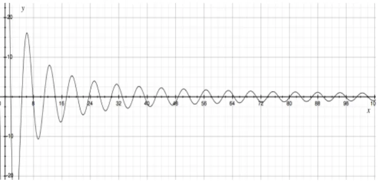
Considering the high impact of external factors, we need to create a controllable experiment aiming to check if the model is generating coherent results. For such task, we had to set an input that we already had an expected output. This dataset, called WaveDS, construction is depicted in Figure 4.

Figure 4: Synthetic dataset, WaveDS.

Clearly, we can see that tending to infinity the value of the wave should be 0. The expected flow for this experiment is the sequence:

1. SAX reads the TS and returns the corresponding sym-bolic data, being “a" the class close to −20 and “j" the class close to 20.

2. The Coder reads the symbolic data, calculate the prob-abilities and creates the stochastic model.

3. The model must return a very high steady state percent-age chance for the classes close to 0.

The three steps had worked as expected; the experiment returns a high percentage values for the steady state in classes “e" and “f" that represents values close to zero, 48.63% and 48.03%, respectively. This experiment shows that the expected sequence was performed and the process has worked as expected.

The same approach was performed for all other datasets. For the synthetic datasets the output match with the expected classes, although 2 in market datasets the expected class was the second and third with higher percentages. This was expected, because there are many fluctuations on the market datasets that are very difficult to predict using only the historical data.

From all datasets tested, we divided nearly 80% to run in our process and 20% to test the output. For the datasets Symbolsand WordsSynonyms, we had no significant changes, i.e., the steady state for all classes was achieved in the very beginning, and the value became close to the original. In Paris Temp dataset, we found two high scores for non adjacent classes, i.e., classes that cannot be agglutinated into one because they are non contiguous. Although, for the other datasets our quantitative analysis was accurate with the test part of the dataset.

All experiments results are show in Table 1. In this table is indicated the name of the dataset, the probabilities of the more frequent classes, and a general indication if the experiment prediction was accurate ("X" indicates an experiment with a correct prediction, i.e., the predicted class, "†" indicates otherwise).

Dataset Predicted probabilities Accuracy Coffee j: 94.28% X Symbols f: 12.51%; g: 11.94% X WordsSynonyms i: 29.51%; j: 29.01% _X ItalyPowerDemand i: 40.21%; j: 42.54% _X petr3 b: 18.68 % _X bbas3 b: 45.37% _X brfs3 b: 55.80% _X vale3 a: 37.30% † Paris Temp c: 21.55%; i: 25.08% † WaveDS e: 48.63%, f: 48.03% _X Table 1: Probabilities and classes found for each dataset ("_{X" indicates accurate and "†" indicates inaccurate).}

For dataset Paris Temp the problem seems related to the bimodal characteristic of the data, since two non adjacent classes (c and i) were the more frequent ones. Dataset vale3, however, seems to be a more complex case and it deserves a deeper analysis in the future.

7 Conclusion

We successfully created a process that drives us into a next step to forecast data with high dimensionally. Our process is capable of making stochastic predictions through Markovian models coping with the curse of dimensionality. Our tests shows that the new process created is useful to reduce the data dimensionality and perform forecasting through stochastic models. Also connecting the best techniques in the literature we were able to automate the steps that usually demands time and effort from specialists.

More than forecasting, this process provides a new way to perform data mining tasks in high dimensional data. Now we are able to use Makovian models to knowledge discovery with a large amount of data, due to the curse of dimensionality it was infeasible before. This brings us to new challenges, once that we have a large amount of algorithms to solve problems using stochastic models.

In the implementation front, the next step is to generate the SAN code through the Coder, thus we can save time performing multiples executions due to the SAN format and the large variety of the algorithms already implemented in the SAN tools [6] [27]. This certainly will bring us more performance to make more tests and use the model into new scenarios, such as big data.

Other possible application is the real time prediction for streaming data. A dimensionality reduction can be applied online generating SAN code to be solved in real time, thus predicting next states.

References

[1] J. ASSUNÇÃO, L. ESPINDOLA, P. FERNANDES, M. PIVEL,

ANDA. SALES, A structured stochastic model for prediction of geological stratal stacking patterns, in 6th Practical Ap-plications of Stochastic Modelling (PASM’12), London, UK, September 2012, pp. 1–15.

[2] J. ASSUNÇÃO, P. FERNANDES, T. FISCHER, AND

A. SALES, Unsupervised model generation for geological events, 2014. Accepted to 46th Annual Simulation Sympo-sium.

[3] J. BERMAN, Principles of Big Data: Preparing, Sharing, and Analyzing Complex Information, Elsevier Science, 2013. [4] G. E. BOX, G. M. JENKINS, ANDG. C. REINSEL, Time

series analysis: forecasting and control, Wiley. com, 2013.

[5] L. BRENNER, P. FERNANDES, J.-M. FOURNEAU, AND

B. PLATEAU, Modelling Grid5000 point availability with SAN, Electronic Notes in Theoretical Computer Science (ENTCS), 232 (2009), pp. 165–178.

[6] L. BRENNER, P. FERNANDES, B. PLATEAU, ANDI. SBE

-ITY, PEPS2007 - Stochastic Automata Networks Software Tool, in Proceedings of the 4th International Conference on Quantitative Evaluation of SysTems (QEST 2007), Ed-inburgh, UK, September 2007, IEEE Computer Society, pp. 163–164.

[7] L. BRENNER, P. FERNANDES, AND A. SALES, The Need for and the Advantages of Generalized Tensor Algebra for Kronecker Structured Representations, International Journal of Simulation: Systems, Science & Technology (IJSIM), 6 (2005), pp. 52–60.

[8] K. CHAKRABARTI, E. KEOGH, S. MEHROTRA, AND

M. PAZZANI, Locally adaptive dimensionality reduction for indexing large time series databases, ACM Trans. Database Syst., 27 (2002), pp. 188–228.

[9] C. CHATFIELD, Time-series forecasting, Chapman and

Hall/CRC, 2002.

[10] R. M. CZEKSTER, P. FERNANDES, J.-M. VINCENT, AND

T. WEBBER, Split: a flexible and efficient algorithm to vector-descriptor product, in International Conference on Perfor-mance Evaluation Methodologies and tools (ValueTools’07), vol. 321 of ACM International Conferences Proceedings Se-ries, ACM Press, 2007, pp. 83–95.

[11] R. M. CZEKSTER, P. FERNANDES, AND T. WEBBER,

Efficient vector-descriptor product exploiting time-memory trade-offs, ACM SIGMETRICS Performance Evaluation Re-view, 39 (2011), pp. 2–9. doi: 10.1145/2160803.2160805. [12] DATAMARKET!, The open portal to thousands of datasets

from leading global providers. http://datamarket.com/, 2013. [13] C. ENGEL, Can the markov switching model forecast ex-change rates?, Journal of International Economics, 36 (1994), pp. 151–165.

[14] P. FERNANDES, M. O’KELLY, C. PAPADOPOULOS, AND

A. SALES, Analysis of exponential reliable production lines using kronecker descriptors, Int. Journal of Production Re-search, 51 (2013), pp. 2511–2528.

[15] P. FERNANDES, B. PLATEAU, ANDW. J. STEWART, Effi-cient descriptor-vector multiplication in Stochastic Automata Networks, Journal of the ACM, 45 (1998), pp. 381–414. [16] P. FERNANDES, A. SALES, A. R. SANTOS, ANDT. WEB

-BER, Performance evaluation of software development teams: a practical case study, Electronic Notes in Theoretical Com-puter Science, 275 (2011), pp. 73 – 92.

[17] J. HAN, M. KAMBER, AND J. PEI, Data Mining, Second Edition: Concepts and Techniques, The Morgan Kaufmann Series in Data Management Systems, Elsevier Science, 2006. [18] E. KEOGH, L. WEI, X. XI, S.-H. LEE,ANDM. VLACHOS, Lb_keogh supports exact indexing of shapes under rotation invariance with arbitrary representations and distance mea-sures, in Proceedings of the 32nd international conference on Very large data bases, VLDB ’06, VLDB Endowment, 2006, pp. 882–893.

[19] E. KEOGH, Q. ZHU, B. HU, Y. HAO, X. XI, L. WEI,

AND RATANAMAHATANA, The UCR Time Series Classifi-cation/Clustering Homepage. www.cs.ucr.edu/~eamonn/ time_series_data/, 2011.

[20] F. KORN, H. V. JAGADISH,ANDC. FALOUTSOS, Efficiently supporting ad hoc queries in large datasets of time sequences, in Proceedings of the 1997 ACM SIGMOD international conference on Management of data, SIGMOD 97, New York, NY, USA, 1997, ACM, pp. 289–300.

[21] J. LIN, E. KEOGH, S. LONARDI,ANDB. CHIU, A symbolic representation of time series, with implications for streaming algorithms, in Proceedings of the 8th ACM SIGMOD

work-shop on Research issues in data mining and knowledge dis-covery, DMKD ’03, New York, NY, USA, 2003, ACM, pp. 2– 11.

[22] Z. LINJESSICA, Y. HUANG, H. WANG,ANDS. MCCLEAN, Neighborhood counting for financial time series forecasting, in Evolutionary Computation, 2009. CEC ’09. IEEE Congress on, 2009, pp. 815–821.

[23] J. PERALTA, G. GUTIERREZ, AND A. SANCHIS, Shuffle design to improve time series forecasting accuracy, in Evo-lutionary Computation, 2009. CEC ’09. IEEE Congress on, 2009, pp. 741–748.

[24] B. PLATEAU, On the stochastic structure of parallelism and synchronization models for distributed algorithms, ACM SIGMETRICS Performance Evaluation Review, 13 (1985), pp. 147–154.

[25] K. PONG CHAN AND A. W.-C. FU, Efficient time series matching by wavelets, in Proceedings of the 15th International Conference on Data Engineering, M. Kitsuregawa, M. P. Papazoglou, and C. Pu, eds., ICDE ’99, Washington, DC, USA, 1999, IEEE Computer Society, pp. 126–133.

[26] R. REYHANI ANDA.-M. MOGHADAM, A heuristic method

for forecasting chaotic time series based on economic vari-ables, in Digital Information Management (ICDIM), 2011 Sixth International Conference on, 2011, pp. 300–304. [27] A. SALES, San lite-solver: a user-friendly software tool to

solve san models, in Proceedings of the 2012 Symposium on Theory of Modeling and Simulation - DEVS Integrative M&S Symposium, TMS/DEVS ’12, San Diego, CA, USA, 2012, Society for Computer Simulation International, pp. 44:9–16. [28] T. STEFFENS ANDP. HUGELMEYER, Real-time prediction

in a stochastic domain via similarity-based data-mining, in Simulation Conference, 2007 Winter, 2007, pp. 1430–1435. [29] W. J. STEWART, Probability, Markov Chains, Queues, and

Simulation, Princeton University Press, USA, 2009.

[30] A. VALMARI, The state explosion problem, in Lectures on Petri Nets I: Basic Models, W. Reisig and G. Rozenberg, eds., vol. 1491 of Lecture Notes in Computer Science, Springer Berlin Heidelberg, 1998, pp. 429–528.

[31] X. WANG, A. MUEEN, H. DING, G. TRAJCEVSKI,

P. SCHEUERMANN,ANDE. KEOGH, Experimental compar-ison of representation methods and distance measures for time series data, Data Mining and Knowledge Discovery, 26 (2013), pp. 275–309.

[32] I. H. WITTEN, E. FRANK,ANDM. A. HALL, Data Mining: Practical Machine Learning Tools and Techniques, Second Edition, The Morgan Kaufmann Series in Data Management Systems, Elsevier Science, 2011.

[33] YAHOO!, Brazilian market stock indices.

http://br.financas.yahoo.com/indices?e=bovespa, 2013. [34] L. YE ANDE. KEOGH, Time series shapelets: a new

prim-itive for data mining, in Proceedings of the 15th ACM SIGKDD international conference on Knowledge discovery and data mining, KDD ’09, New York, NY, USA, 2009, ACM, pp. 947–956.

[35] G. YU, J. HU, C. ZHANG, L. ZHUANG, AND J. SONG, Short-term traffic flow forecasting based on markov chain model, in Intelligent Vehicles Symposium, 2003. Proceed-ings. IEEE, 2003, pp. 208–212.