Non-Fully Invested Derivative-Free
Bond Index Replication
Iliya Markov, MSc
Research assistant at Haute Ecole de Gestion de Genève
Campus de Battelle, Bâtiment F, 7 route de Drize, 1227 Carouge, Switzerland E-mail: [email protected]
Rodrigue Oeuvray, PhD
Investment risk manager at Pictet Asset Management 10 Merle d'Aubigné, 1207 Geneva, Switzerland E-mail: [email protected]
Nils S. Tuchschmid, PhD Partner at Tages Capital LLP
100 Pall Mall, London, SW1Y 5NQ, United Kingdom E-mail: [email protected]
Abstract: The problem we address here is the replication of a bond benchmark when only a fraction of the portfolio is invested for the replication. Our methodology is based on a minimization of the tracking error subject to a set of constraints, namely (1) the fraction invested for the replication, (2) a no short selling constraint, and (3) a null active duration constraint, where the last one can be relaxed. The constraints can also be adapted to accommodate the use of interest rate and bond futures. Our main contribution, however, lies in the derivative-free approach to replication. It is very useful for managing assets when the use of derivatives is prohibited, for instance by certain investors. We can thus still benefit from replicating a traditional investment in a bond index with a fraction of the portfolio according to our risk appetite. The rest of the portfolio can be invested in alpha-portable strategies. An analysis without the use of derivatives over a period spanning from 1 January 2008 to 3 October 2011 shows that for 70% to 90% invested for the replication the annualized ex-ante tracking error can range from 0.41% to 0.07%. We use principal component analysis to extract the main drivers of the size of the tracking error, namely the volatility of and the differential between the yields in the objective function’s covariance matrix of spot rates. These results highlight our contribution of a generic and intuitive yet robust approach to bond index replication.
Keywords: bond index replication; derivatives; tracking error; optimization JEL Classifications: C61; G11; G24
Published in Financial markets and portfolio management , march 2013,
vol.27, no. 1, p.101-124 which should be cited to refer to this work
2
1. Introduction
The problem we address here is the replication of a government bond benchmark with the constraint that only a fraction of the portfolio is invested for the replication. We assume that the rest of the portfolio is invested in cash, i.e. it does not add to the variation of our investment. Realistically, however, the rest of the portfolio could be invested in an alpha-portable strategy. Derivatives may be used for the replication and we present a case study with Eurodollar interest rate futures and bond futures. However, since we deem replication without the use of derivatives more interesting from a research point of view, we present a rolling analysis of the replication without their use. Moreover, from a practical point of view, certain investors may not allow the use of derivatives. We are interested therefore in the evolution of the ex-ante tracking error (TE) over a sample period from 1 January 2008 to 3 October 2011 assuming that the use of derivatives is not allowed.
In order to determine the optimal replicating portfolio we apply an optimization algorithm that minimizes the TE of the replication under the imposition of several constraints – (1) a cash constraint stating what fraction of the portfolio is invested for the replication, (2) a no short selling constraint implying that we can only take long positions and a (3) null active duration1 constraint establishing that the portfolio duration should be equal to the benchmark duration. We also consider a variation of the problem where the null active duration constraint is relaxed.
As expected, the results of the analysis show that the TE grows as the fraction of the portfolio invested for the replication is reduced. The TE is moreover higher if interest rate and bond futures are not used. Nevertheless, our rolling analysis without the use of derivatives over the period 1 January 2008 to 3 October 2011 shows that for 70% invested for the replication, the annualized ex-ante TE is 0.59% when the duration constraint is imposed and 0.41% when it is not. These are small variations indeed, and allow for the remaining 30% of the portfolio to be deployed in alternative strategies. Moreover, depending on the client’s preferences, larger fractions can be invested for the replication which would further reduce the TE. For 90%, the annualized ex-ante TE is 0.13% when the duration constraint is imposed and 0.07% when it is not. We also use principal component analysis to extract the main determinant of the size of the TE. These are the volatility of the spot rates in the objective function’s covariance matrix and their differentials. Our results highlight the important contribution of the derivative-free approach to bond index replication.
This article is structured as follows. In section 2, we present a short overview of existing literature on bond index replication. In section 3, we offer several formulations of the problem with respect to the use of derivatives and the imposition of the duration constraint. We describe our data in section 4, which is followed by a case study in section 5 with and without derivatives. Section 6 continues with a presentation of the evolution of the TE over the sample period without the use of derivatives. Furthermore, we analyze the evolution of the tracking error through principal component analysis of the objective function’s covariance matrix. Finally, section 7 offers some concluding remarks.
3
2. Brief Review of Related Literature
Modern portfolio theory was introduced by Markowitz (1952) and is one of the pillars of asset management. The adoption of the mean-variance model for bond portfolio selection was first addressed by Cheng (1962) and a major breakthrough came with the work of Vasicek (1977) who was the first to introduce a dynamic term structure model. Wilhelm (1992) admits the practical infeasibility of the dynamic term structure model and uses a mean-variance framework with the bond market defined by the term structure model proposed by Cox, Ingersoll and Ross (1985). Elton et al. (2002) also use modern portfolio theory for the bond selection problem.
Korn and Koziol (2006) study the historical performance of efficient mean-variance German government bond portfolios. They explore investments in bonds of various maturities with the underlying market characterized by an affine term structure model. Puhle (2008) provides an overview of existing bond portfolio optimization literature and derives many of the principal algorithms hitherto mentioned. As regards index replication specifically, several recent studies approach the problem with the use of derivatives. Dynkin et al. (2002) discuss strategies based on Eurodollar futures, Treasury futures, and swaps for the hedging and replication of diversified fixed-income portfolios. They find that the optimal replication portfolios consist of a combination of Treasury futures, Eurodollar futures and swaps. They moreover find that after 1998 tracking errors have become significantly higher. In a related subsequent study Dynkin et al. (2006) point that the demand for alpha-portable strategies has led to increased interest in the replication of fixed-income portfolios via derivatives. For this purpose, beta is generated through unfunded derivatives exposure and the cash is deployed in alpha strategies. They show that using liquid derivatives in different markets leads to tracking error volatility of only 6–9 bps per month.
Given that there are a number of studies having discussed the bond index replication problem with derivatives, the main contribution of our model is a generic approach which provides the flexibility of including or not including derivatives and tackles the replication problem by investing only a fraction of the portfolio. This article therefore aims at contributing to the existing literature by constructing a framework allowing investors with specific requirements, such as no use of derivatives, a way to replicate an index with a fraction of the portfolio and use remaining cash for alternative strategies.
3. Problem Formulation
Our benchmark consists of government bonds with expiration dates from less than 1 to more than 20 years into the future. The number of different securities in the benchmark varies from approximately 130 at the beginning of the sample period to approximately 200 at the end of the sample period. Our strategy consists of decomposing the benchmark into seven buckets2 based on expiration. In the benchmark, each bucket has a certain weight and we refer to these weights as the benchmark weights. Each bucket has a key rate duration (KRD) calculated as the weighted duration of all the papers that comprise it where their benchmark weights are scaled to add up to one for each bucket.
2 Bucketing is explained in section 4.
4
In order to replicate the benchmark, we invest a fraction of the original portfolio in some or all of the buckets. We refer to these new weights invested for the replication as the portfolio weights. The differences between the portfolio weights and the benchmark weights are the active weights of the buckets. We define as the vector of active weights and as the vector of key rate durations of the buckets. The daily tracking difference of the replicating portfolio against the benchmark is:
where is a diagonal matrix where the entries along the main diagonal are the key rate durations of the buckets and is the vector of daily changes of yield to maturity spot rates that proxy the buckets. The multiplication produces in essence a transposed vector of active weighted key rate durations. The daily tracking variance of the replicating portfolio becomes:
Now we have all the ingredients to formulate the problem as a quadratic optimization. We seek to find the vector of active weights that minimizes the tracking error (TE) subject to a set of constraints. The objective function is:
Minimize: ( )
To be precise, the objective function signifies the minimization of the tracking variance induced by the active weights in bond positions. By definition, the TE is the square root of the tracking variance. Therefore, minimizing the tracking variance in effect minimizes the TE. The objective function is the same for all alternative formulations of the problem. In terms of constraints, the formulations will differ depending on whether derivatives are used and whether the null active duration constraint is imposed.
3.1. Problem formulation without derivatives
Without the use of derivatives, we first consider the case where the null active duration constraint is imposed. In this case we have three optimization constraints. The first one concerns the sum of the active weights. By default, the sum of the benchmark weights of all buckets is 100%. Let’s assume that we want to invest only 30% of the portfolio for the replication of the benchmark. In this case, the sum of the active weights for bond positions will be minus 70% as the active weights are the differences between the portfolio weights and the benchmark weights. Therefore, if we impose that we invest only a fraction of the portfolio for the replication, then the first constraint becomes:
5 ∑
where is taken over all buckets. The second constraint concerns the duration of the portfolio. We want that the duration of the replicating portfolio match the duration of the benchmark. Concretely, we want that the sum of the portfolio weighted KRDs be equal to the duration of the benchmark:
where is the vector of portfolio weights and is the duration of the benchmark. The above equation rewrites as:
where this time the vector of portfolio weights is expressed as the sum of the vector of active weights and the vector of benchmark weights . After a few manipulations, we obtain:
Finally, we formulate the second constraint as:
which states that the sum of the active weighted KRDs, or in other words the active duration of the portfolio, is null.
The third constraint imposes that the weights of the portfolio be positive or null, i.e. we are only allowed to take long positions in the buckets. The condition is:
which, after decomposing portfolio weights into active weights and benchmark weights, becomes:
6
Finally, we have the following formulation of the optimization problem:
Problem 1a:
Minimize: ( ) Subject to: ∑ (cash constraint)
(null active duration constraint) (no short selling constraint)
where is taken over all buckets. In terms optimization, imposing a null active duration in the form of an additional constraint may lead to larger TE due to reduction in flexibility. In an alternative formulation of the problem we relax the null active duration constraint:
Problem 1b:
Minimize: ( ) Subject to: ∑ (cash constraint)
(no short selling constraint)
where is taken over all buckets.
3.2. Problem formulation with derivatives
Interest rate derivatives are common in the management of fixed-income portfolios. In our framework we express their exposures in terms of key rates durations (KRD), positive or negative. In replicating a benchmark composed only of government securities it is natural to consider the inclusion of bond futures (to reproduce the exposure of medium and long-term maturity bonds) and possibly Eurodollar futures (typically to reproduce the short-term exposure of Treasury bills). For a bond futures, we would consider that its exposure is given by the duration of the cheapest-to-deliver (CTD) bond (after adjustment for the conversion factor) while for a Eurodollar futures we would simply consider the KRD.
Indeed, we model a bond futures as an investment in the CTD bond. So the output of our algorithm is the weight invested in the CTD bond. Note that by doing so, we ignore the basis between bonds and futures. The weight of the CTD bond, however, can easily be converted into a number of bond futures if necessary. To further simplify modeling, we also make the assumption that we invest only via derivatives in their maturity buckets. For example, if we use a 10Y bond futures whose CTD bond matures in say the [6Y – 8.5Y] bucket, then we invest in this bucket only via bond futures and not bonds for the replication of the benchmark. Therefore, we replace the original cash constraint:
7 ∑
where is taken over all buckets, by a new cash constraint of the form:
∑ ∑
where this time is taken over all buckets except the Eurodollar bucket and the CTD bond bucket. We moreover relax the no short selling constraint for the derivative buckets.
When the null active duration constraint is imposed, we obtain the following formulation:
Problem 2a:
Minimize: ( ) Subject to: ∑ ∑ (cash constraint)
(null active duration constraint) (no short selling constraint)
where is taken over all buckets except the Eurodollar bucket and the CTD bond bucket. Relaxing the null active duration constraint, we obtain the alternative formulation below:
Problem 2b:
Minimize: ( ) Subject to: ∑ ∑ (cash constraint)
(no short selling constraint)
where is taken over all buckets except the Eurodollar bucket and the CTD bond bucket.
4. Data
The bond benchmark we use is the JP Morgan Global Bonds Index All Maturities in Local Currency, available in Bloomberg (JPMTUS Index). It is taken at the beginning of each month from 1 January 2008 to 3 October 2011, i.e. the sample period spans 46 months in total. In the cases where valuation of the benchmark is not possible on the 1st of the month, we take the nearest date after the beginning of the month where there is a valuation for the benchmark.
8
In order to calculate the covariance matrix in the objective function, we use the USGG daily spot rates available in Bloomberg (GGR: Global Generic Government Rates). The rates are yields to maturity (pre-tax) and are available for 10 maturities – 1M, 3M, 6M, 1Y, 2Y, 3Y, 5Y, 7Y, 10Y and 30Y. Over our sample period, the benchmark does not contain papers expiring in less than 9 months. Therefore, for the purposes of our optimization we have only used the USGG rates with maturities of 1Y and above.
For each date that the benchmark is taken on, we bucket its papers by expiration into seven buckets. The buckets are then proxied by the USGG rates. Since it is not always possible for the rates to fall in the middle of each bucket, we use a rule where the buckets are constructed so the average maturity of every pair of adjacent USGG rates defines the bucket boundaries as shown in table 1 below.
Table 1 Benchmark buckets and USGG proxy rates
This table presents the bucketing of the benchmark papers and the USGG rates that proxy the respective buckets.
Benchmark buckets USGG proxy rates
[0Y – 1.5Y] 1Y
[1.5Y – 2.5Y] 2Y
[2.5Y – 4Y] 3Y
[4Y – 6Y] 5Y
[6Y – 8.5Y] 7Y
[8.5Y – 20Y] 10Y
[+20Y] 30Y
As mentioned above, the USGG rates are used for the calculation of the covariance matrix in the objective function. For each date that the benchmark is taken on, we use the preceding 260 daily rate changes for the calculation of the covariances. The latter is due the fact that there are approximately 260 daily rate changes in a year.
As a result, the sample period of the USGG rates is from 1 January 2007 (i.e. 1 year prior to the first benchmark date) to 3 October 2011. In some cases there are missing data for some of the rates (particularly the 1Y and the 7Y rates which start reporting at a later date). To amend the problem we have interpolated the missing values using piecewise cubic Hermite interpolation. In interpolating the missing values we have used all available rates (not just those with maturities of 1Y and above) in order to obtain maximum precision.
We should mention that by default the covariance matrix is positive semi-definite and as such may cause problems for the optimization algorithm which requires a positive definite matrix as an input. In case the covariance matrix is not positive definite we could have numerical problems as we use a solver for strictly convex programs. There are workarounds in such cases, for example the algorithm of Higham (1988), which can be used to compute the nearest positive definite of a real symmetric matrix. Fortunately, however, over our sample period and for our data, the covariance matrix is always positive definite.
9
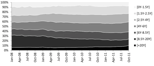
Figure 1 below presents the evolution of the benchmark weights by buckets over our sample period from 1 January 2008 to 3 October 2011.
Fig. 1 Benchmark weights
This figure presents the evolution of the benchmark weights by buckets over the sample period from 1 January 2008 to 3 October 2011.
Overall, we observe that the weight of the [8.5Y-20Y] bucket decreases substantially over the course of our sample period. The benchmark weights of the shortest term buckets ([0Y-1.5Y] and [1.5Y-2.5Y]) remain almost constant. The benchmark weights of the rest of the buckets exhibit slight increase. Figure 2 below presents the benchmark weighted key rate durations (KRD) of the buckets.
Fig. 2 Benchmark weighted key rate durations
This figure presents the evolution of the benchmark weighted key rate durations of the buckets over the sample period from 1 January 2008 to 3 October 2011.
0% 10% 20% 30% 40% 50% 60% 70% 80% 90% 100% Jan -08 Ap r-08 Ju l-08 Oct-08 Jan -09 Ap r-09 Ju l-09 Oc t-09 Jan -10 Ap r-10 Ju l-10 Oct-10 Jan -11 Ap r-11 Ju l-11 Oct-11 [0Y-1.5Y] [1.5Y-2.5Y] [2.5Y-4Y] [4Y-6Y] [6Y-8.5Y] [8.5Y-20Y] [+20Y] 0 0.5 1 1.5 2 2.5 Jan -08 Ap r-08 Ju l-08 Oc t-08 Jan -09 Ap r-09 Ju l-09 Oc t-09 Jan -10 Ap r-10 Ju l-10 Oc t-10 Jan -11 Ap r-11 Ju l-11 Oc t-11 [0Y-1.5Y] [1.5Y-2.5Y] [2.5Y-4Y] [4Y-6Y] [6Y-8.5Y] [8.5Y-20Y] [+20Y]
10
As figure 2 shows, the benchmark weighted KRD of the [8.5Y-20Y] bucket undergoes a substantial decrease over the course of the sample period. The benchmark weighted KRD of the rest of the buckets remain more or less the same or show slight increase. Only the benchmark weighted KRD of the [+20Y] bucket increases more substantially, especially at the end of the sample period.
5. Case Study
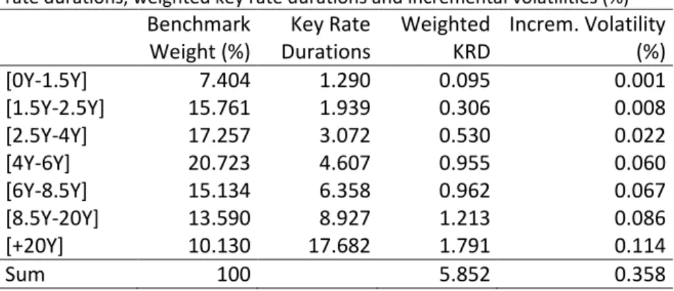
The case study below is focused on the benchmark as taken on 3 October 2011, i.e. at the end of the sample period. Table 2 below presents some statistics of the benchmark for this particular date. As the table shows, it is predominantly composed of papers of short to medium-term maturities and its modified duration is 5.852.
Table 2 Benchmark statistics on 3 October 2011
This table presents benchmark statistics in terms of bucket weights (%), key rate durations, weighted key rate durations and incremental volatilities (%)
Benchmark Weight (%) Key Rate Durations Weighted KRD Increm. Volatility (%) [0Y-1.5Y] 7.404 1.290 0.095 0.001 [1.5Y-2.5Y] 15.761 1.939 0.306 0.008 [2.5Y-4Y] 17.257 3.072 0.530 0.022 [4Y-6Y] 20.723 4.607 0.955 0.060 [6Y-8.5Y] 15.134 6.358 0.962 0.067 [8.5Y-20Y] 13.590 8.927 1.213 0.086 [+20Y] 10.130 17.682 1.791 0.114 Sum 100 5.852 0.358
The subsections below analyze the replication of the benchmark on 3 October 2011 for different fractions of the portfolio invested for the replication. First we consider replication without the use of derivatives and then with the use of derivatives.
In all of the analyses we calculate the annualized ex-ante tracking error. The objective function in the optimization algorithm designates the daily tracking variance (i.e. the square of the daily tracking error). Therefore, to obtain the daily tracking error we take the square root of the value of the objective function after each optimization. We then annualize it by multiplying it by the square root of 260, where 260 is the approximate number of days in a year. We call this an annualized ex-ante tracking error as opposed to an ex-post or realized tracking error. An ex-post tracking error is impossible to calculate in our case as we do not have the ex-post performance of the benchmark and our fictitious portfolios. The annualized ex-ante tracking error is henceforth for brevity referred to simply as the tracking error (TE).
11 5.1. Replication without derivatives
Tables 3 to 5 below present the portfolio weights, the active weights and the active weighted durations respectively when various fractions of the portfolio are invested for the replication and the duration constraint is imposed (Problem 1a). Since imposing that the active duration be null translates into a significant reduction in flexibility, the optimization algorithm has no solution for small fractions. In the tables below, the optimization produces a solution for 40% and more of the portfolio invested for the replication.
As is evident, investing smaller fractions favors those buckets that contribute the most to the volatility of the benchmark (see Incremental Volatility, table 2 above). When only 40% is invested, the portfolio populates the [8.5Y-20Y] and the [+20Y] buckets which have the highest incremental volatilities. Investing a higher fraction successively populates the buckets with lower incremental volatilities. As expected, investing a higher fraction substantially reduces the TE as well.
Table 3 Portfolio weights (%) without derivatives; with duration constraint (Problem 1a)
This table presents the portfolio weights (%) for various fractions of the portfolio invested for the replication without the use of derivatives but with duration constraint. Benchmark taken on 3 October 2011.
Benchmark Weight % = 1% = 10% = 20% = 30% = 40% = 70% = 90% [0Y-1.5Y] 7.404 -- -- -- -- -- -- -- [1.5Y-2.5Y] 15.761 -- -- -- -- -- -- 3.78 [2.5Y-4Y] 17.257 -- -- -- -- -- -- 28.51 [4Y-6Y] 20.723 -- -- -- -- -- 25.84 19.13 [6Y-8.5Y] 15.134 -- -- -- -- -- 19.64 14.73 [8.5Y-20Y] 13.590 -- -- -- -- 13.94 10.53 12.93 [+20Y] 10.130 -- -- -- -- 26.06 13.99 10.92 Ann. Ex-Ante TE (%) -- -- -- -- 2.02 0.63 0.12
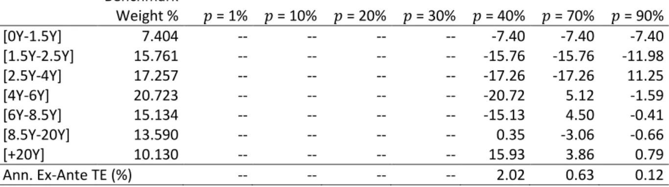
Table 4 Active weights (%) without derivatives; with duration constraint (Problem 1a)
This table presents the active weights (%) for various fractions of the portfolio invested for the replication without the use of derivatives but with duration constraint. Benchmark taken on 3 October 2011.
Benchmark Weight % = 1% = 10% = 20% = 30% = 40% = 70% = 90% [0Y-1.5Y] 7.404 -- -- -- -- -7.40 -7.40 -7.40 [1.5Y-2.5Y] 15.761 -- -- -- -- -15.76 -15.76 -11.98 [2.5Y-4Y] 17.257 -- -- -- -- -17.26 -17.26 11.25 [4Y-6Y] 20.723 -- -- -- -- -20.72 5.12 -1.59 [6Y-8.5Y] 15.134 -- -- -- -- -15.13 4.50 -0.41 [8.5Y-20Y] 13.590 -- -- -- -- 0.35 -3.06 -0.66 [+20Y] 10.130 -- -- -- -- 15.93 3.86 0.79 Ann. Ex-Ante TE (%) -- -- -- -- 2.02 0.63 0.12
12
Table 5 Active weighted durations without derivatives; with duration constraint (Problem 1a)
This table presents the active weighted durations for various fractions of the portfolio invested for the replication without the use of derivatives but with duration constraint. Benchmark taken on 3 October 2011.
Bench Wtd. KRD = 1% = 10% = 20% = 30% = 40% = 70% = 90% [0Y-1.5Y] 0.095 -- -- -- -- -0.10 -0.10 -0.10 [1.5Y-2.5Y] 0.306 -- -- -- -- -0.31 -0.31 -0.23 [2.5Y-4Y] 0.530 -- -- -- -- -0.53 -0.53 0.35 [4Y-6Y] 0.955 -- -- -- -- -0.95 0.24 -0.07 [6Y-8.5Y] 0.962 -- -- -- -- -0.96 0.29 -0.03 [8.5Y-20Y] 1.213 -- -- -- -- 0.03 -0.27 -0.06 [+20Y] 1.791 -- -- -- -- 2.82 0.68 0.14 Ann. Ex-Ante TE (%) -- -- -- -- 2.02 0.63 0.12
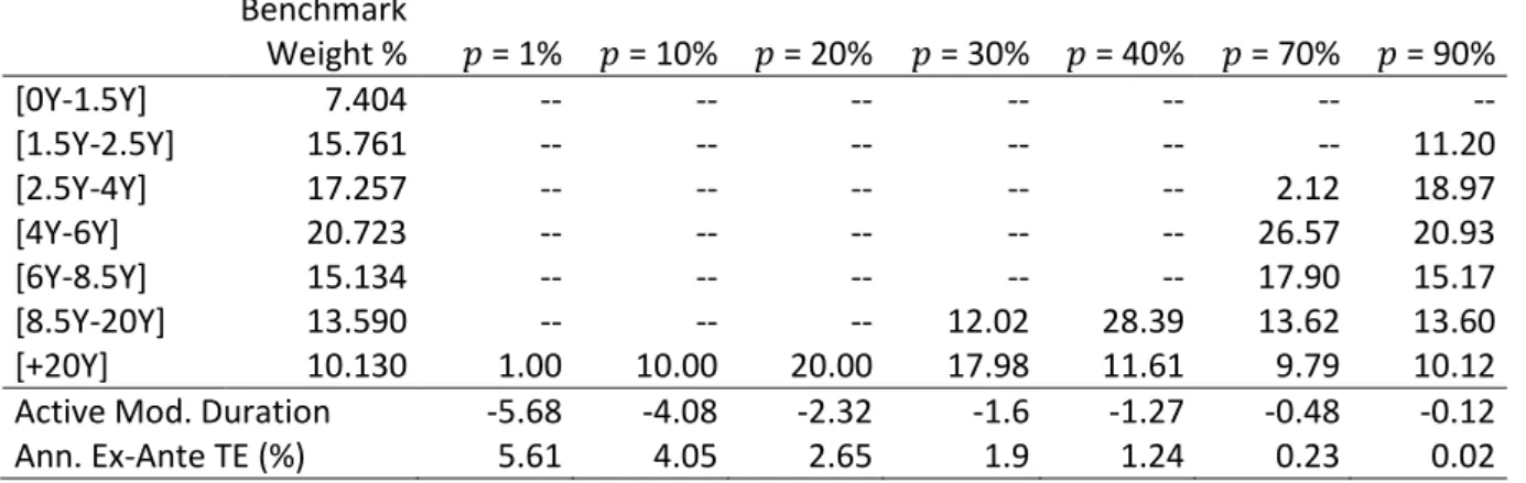
Tables 6 to 8 below present the portfolio weights, the active weights and the active weighted durations respectively when various fractions of the portfolio are invested for the replication and the duration constraint is relaxed (Problem 1b). For small fractions, the portfolio again favors those buckets that have high incremental volatilities. For higher fractions, the portfolio successively populates the buckets with lower incremental volatilities. Unlike in the case above, this time the optimization produces results for any fraction. The portfolio also invests with lower active weights in the long-term buckets thus reducing the impact of their high durations. As a result, the active duration of the portfolio is negative and the TE is lower for 40%, 70% and 90%. The TE is again reduced as higher fractions are invested for the replication.
Table 6 Portfolio weights (%) without derivatives; without duration constraint (Problem 1b)
This table presents the portfolio weights (%) for various fractions of the portfolio invested for the replication without the use of derivatives and without duration constraint. Benchmark taken on 3 October 2011.
Benchmark Weight % = 1% = 10% = 20% = 30% = 40% = 70% = 90% [0Y-1.5Y] 7.404 -- -- -- -- -- -- -- [1.5Y-2.5Y] 15.761 -- -- -- -- -- -- 11.20 [2.5Y-4Y] 17.257 -- -- -- -- -- 2.12 18.97 [4Y-6Y] 20.723 -- -- -- -- -- 26.57 20.93 [6Y-8.5Y] 15.134 -- -- -- -- -- 17.90 15.17 [8.5Y-20Y] 13.590 -- -- -- 12.02 28.39 13.62 13.60 [+20Y] 10.130 1.00 10.00 20.00 17.98 11.61 9.79 10.12
Active Mod. Duration -5.68 -4.08 -2.32 -1.6 -1.27 -0.48 -0.12
13
Table 7 Active weights (%) without derivatives; without duration constraint (Problem 1b)
This table presents the active weights (%) for various fractions of the portfolio invested for the replication without the use of derivatives and without duration constraint. Benchmark taken on 3 October 2011.
Benchmark Weight % = 1% = 10% = 20% = 30% = 40% = 70% = 90% [0Y-1.5Y] 7.404 -7.40 -7.40 -7.40 -7.40 -7.40 -7.40 -7.40 [1.5Y-2.5Y] 15.761 -15.76 -15.76 -15.76 -15.76 -15.76 -15.76 -4.56 [2.5Y-4Y] 17.257 -17.26 -17.26 -17.26 -17.26 -17.26 -15.14 1.71 [4Y-6Y] 20.723 -20.72 -20.72 -20.72 -20.72 -20.72 5.84 0.21 [6Y-8.5Y] 15.134 -15.13 -15.13 -15.13 -15.13 -15.13 2.77 0.04 [8.5Y-20Y] 13.590 -13.59 -13.59 -13.59 -1.57 14.80 0.03 0.01 [+20Y] 10.130 -9.13 -0.13 9.87 7.85 1.48 -0.34 -0.01
Active Mod. Duration -5.68 -4.08 -2.32 -1.60 -1.27 -0.48 -0.12
Ann. Ex-Ante TE (%) 5.61 4.05 2.65 1.90 1.24 0.23 0.02
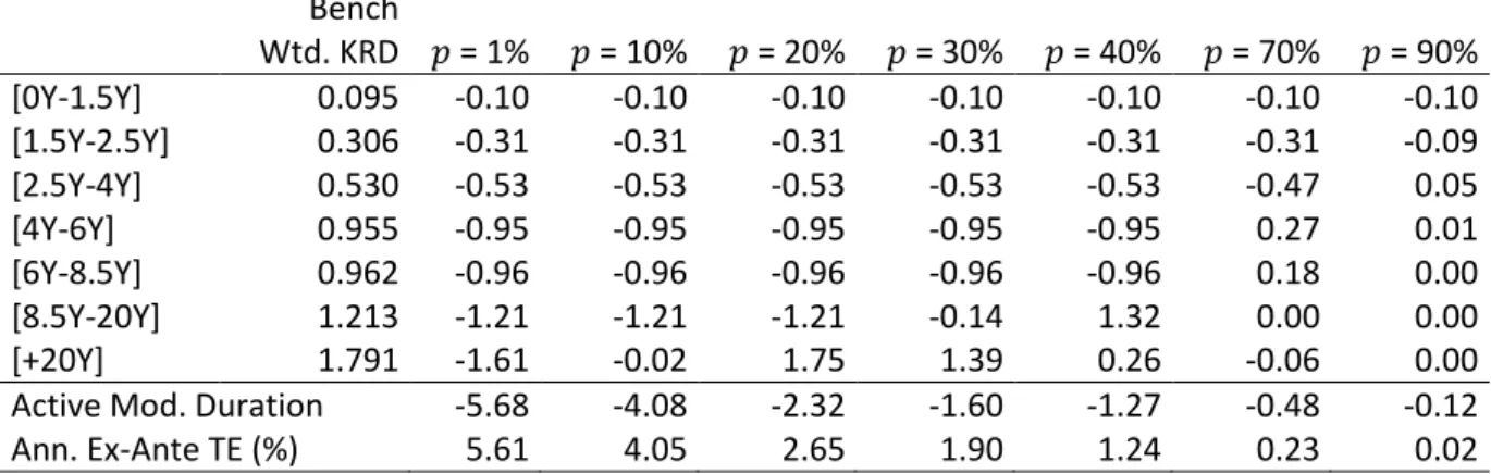
Table 8 Active weighted durations without derivatives; without duration constraint (Problem 1b)
This table presents the active weighted durations for various fractions of the portfolio invested for the replication without the use of derivatives and without duration constraint. Benchmark taken on 3 October 2011. Bench Wtd. KRD = 1% = 10% = 20% = 30% = 40% = 70% = 90% [0Y-1.5Y] 0.095 -0.10 -0.10 -0.10 -0.10 -0.10 -0.10 -0.10 [1.5Y-2.5Y] 0.306 -0.31 -0.31 -0.31 -0.31 -0.31 -0.31 -0.09 [2.5Y-4Y] 0.530 -0.53 -0.53 -0.53 -0.53 -0.53 -0.47 0.05 [4Y-6Y] 0.955 -0.95 -0.95 -0.95 -0.95 -0.95 0.27 0.01 [6Y-8.5Y] 0.962 -0.96 -0.96 -0.96 -0.96 -0.96 0.18 0.00 [8.5Y-20Y] 1.213 -1.21 -1.21 -1.21 -0.14 1.32 0.00 0.00 [+20Y] 1.791 -1.61 -0.02 1.75 1.39 0.26 -0.06 0.00
Active Mod. Duration -5.68 -4.08 -2.32 -1.60 -1.27 -0.48 -0.12
Ann. Ex-Ante TE (%) 5.61 4.05 2.65 1.90 1.24 0.23 0.02
5.2. Replication with derivatives
Below we perform an analysis analogous to the above by allowing the use of derivatives. We use two types of derivatives – Eurodollar interest rate futures and 10Y bond futures. To include Eurodollar futures we relax the no short selling constraint for the shortest-term bucket [0Y-1.5Y]. The 10Y bond futures are modeled as the cheapest-to-deliver (CTD) bond available on 3 October 2011. The CTD bond expires on 15 August 2018 which translates into 6.87 years to expiration. The CTD bond is therefore bucketed in the [6Y-8.5Y] bucket. Its modified duration of 6.082 replaces the KRD of the [6Y-8.5Y] bucket which is 6.358. In addition, we relax the no short selling constraint for this bucket as well. We also use the modified cash constraint which does not count the derivatives buckets.
Tables 9 to 11 below present the portfolio weights, the active weights and the active weighted durations respectively when various fractions of the portfolio invested for the replication and the duration constraint is imposed (Problem 2a). Unlike in the cases where the duration constraint is
14
imposed without the use of derivatives, here there are solutions for any fraction. The latter is due to the flexibility allowed by the use of derivatives. As is evident, the portfolio invests heavily in Eurodollar futures and 10Y bond futures when small fractions of the portfolio are invested. As the fraction grows, we see that the portfolio gradually populates the buckets with higher incremental volatilities and invests less in derivatives.
Moreover, we see a substantial reduction of the TE compared to when derivatives are not used. A detail worth mentioning is that the TE is higher when 90% is invested compared to when 70% is invested for the replication. When 90% is invested, the portfolio has a short position in Eurodollar futures.
Table 9 Portfolio weights (%) with derivatives; with duration constraint (Problem 2a)
This table presents the portfolio weights (%) for various fractions of the portfolio invested for the replication with the use of derivatives and with duration constraint. Benchmark taken on 3 October 2011.
Benchmark Weight % = 1% = 10% = 20% = 30% = 40% = 70% = 90% [0Y-1.5Y]a 7.404 79.75 53.29 46.41 39.91 33.66 13.41 -2.69 [1.5Y-2.5Y] 15.761 -- -- -- -- -- 8.31 28.28 [2.5Y-4Y] 17.257 -- -- 0.51 5.44 10.32 18.97 14.39 [4Y-6Y] 20.723 -- -- 8.56 11.16 13.60 19.85 22.18 [6Y-8.5Y]b 15.134 75.72 55.17 47.18 40.64 33.97 17.20 11.67 [8.5Y-20Y] 13.590 -- -- -- 2.58 5.45 12.68 15.13 [+20Y] 10.130 1.00 10.00 10.93 10.81 10.64 10.19 10.03 Ann. Ex-Ante TE (%) 1.18 0.45 0.37 0.29 0.22 0.04 0.06
a We invest in this bucket via Eurodollar futures b We invest in this bucket via 10Y bond futures
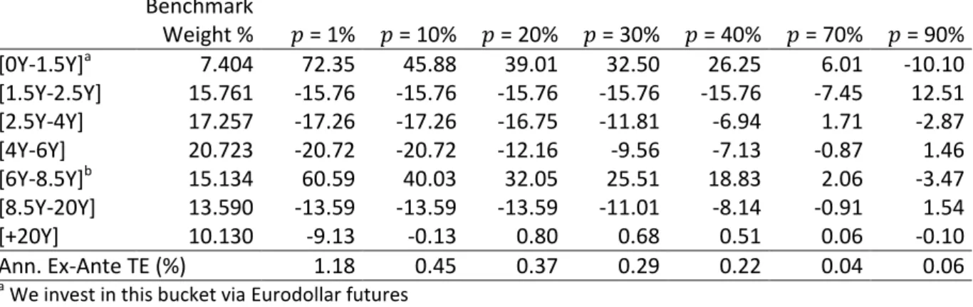
Table 10 Active weights (%) with derivatives; with duration constraint (Problem 2a)
This table presents the active weights (%) for various fractions of the portfolio invested for the replication with the use of derivatives and with duration constraint. Benchmark taken on 3 October 2011.
Benchmark Weight % = 1% = 10% = 20% = 30% = 40% = 70% = 90% [0Y-1.5Y]a 7.404 72.35 45.88 39.01 32.50 26.25 6.01 -10.10 [1.5Y-2.5Y] 15.761 -15.76 -15.76 -15.76 -15.76 -15.76 -7.45 12.51 [2.5Y-4Y] 17.257 -17.26 -17.26 -16.75 -11.81 -6.94 1.71 -2.87 [4Y-6Y] 20.723 -20.72 -20.72 -12.16 -9.56 -7.13 -0.87 1.46 [6Y-8.5Y]b 15.134 60.59 40.03 32.05 25.51 18.83 2.06 -3.47 [8.5Y-20Y] 13.590 -13.59 -13.59 -13.59 -11.01 -8.14 -0.91 1.54 [+20Y] 10.130 -9.13 -0.13 0.80 0.68 0.51 0.06 -0.10 Ann. Ex-Ante TE (%) 1.18 0.45 0.37 0.29 0.22 0.04 0.06 a
We invest in this bucket via Eurodollar futures
15
Table 11 Active weighted durations with derivatives; with duration constraint (Problem 2a)
This table presents the active weighted durations for various fractions of the portfolio invested for the replication with the use of derivatives and with duration constraint. Benchmark taken on 3 October 2011.
Bench Wtd. KRD = 1% = 10% = 20% = 30% = 40% = 70% = 90% [0Y-1.5Y]a 0.095 0.93 0.59 0.50 0.42 0.34 0.08 -0.13 [1.5Y-2.5Y] 0.306 -0.31 -0.31 -0.31 -0.31 -0.31 -0.14 0.24 [2.5Y-4Y] 0.530 -0.53 -0.53 -0.51 -0.36 -0.21 0.05 -0.09 [4Y-6Y] 0.955 -0.95 -0.95 -0.56 -0.44 -0.33 -0.04 0.07 [6Y-8.5Y]b 0.920 3.68 2.43 1.95 1.55 1.15 0.13 -0.21 [8.5Y-20Y] 1.213 -1.21 -1.21 -1.21 -0.98 -0.73 -0.08 0.14 [+20Y] 1.791 -1.61 -0.02 0.14 0.12 0.09 0.01 -0.02 Ann. Ex-Ante TE (%) 1.18 0.45 0.37 0.29 0.22 0.04 0.06
a We invest in this bucket via Eurodollar futures b
We invest in this bucket via 10Y bond futures; CTD bond duration replaces benchmark duration
Tables 12 to 14 present the portfolio weights, the active weights and the active weighted durations respectively when the duration constraint is relaxed (Problem 2b). Compared to when the duration constraint is imposed, we see a negligible drop in the TE. For 70% and 90% invested for the replication, the active duration of the portfolio is close to zero, but the portfolio invests in the buckets in a slightly different manner compared to when the duration is explicitly imposed. When 90% is invested for the replication, we still have a short position in Eurodollar futures.
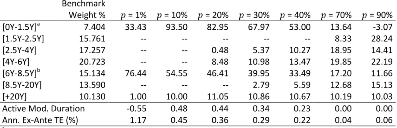
Table 12 Portfolio weights (%) with derivatives; without duration constraint (Problem 2b)
This table presents the portfolio weights (%) for various fractions of the portfolio invested for the replication with the use of derivatives but without duration constraint. Benchmark taken on 3 October 2011.
Benchmark Weight % = 1% = 10% = 20% = 30% = 40% = 70% = 90% [0Y-1.5Y]a 7.404 33.43 93.50 82.95 67.97 53.00 13.64 -3.07 [1.5Y-2.5Y] 15.761 -- -- -- -- -- 8.33 28.24 [2.5Y-4Y] 17.257 -- -- 0.48 5.37 10.27 18.95 14.41 [4Y-6Y] 20.723 -- -- 8.48 10.98 13.47 19.85 22.19 [6Y-8.5Y]b 15.134 76.44 54.55 46.41 39.95 33.49 17.20 11.66 [8.5Y-20Y] 13.590 -- -- -- 2.79 5.59 12.68 15.13 [+20Y] 10.130 1.00 10.00 11.05 10.86 10.67 10.19 10.03
Active Mod. Duration -0.55 0.48 0.44 0.34 0.23 0.00 0.00
Ann. Ex-Ante TE (%) 1.17 0.45 0.36 0.29 0.22 0.04 0.06
a
We invest in this bucket via Eurodollar futures
b
16
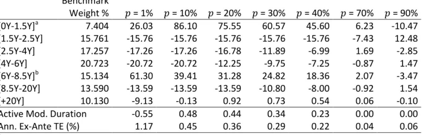
Table 13 Active weights (%) with derivatives; without duration constraint (Problem 2b)
This table presents the active weights (%) for various fractions of the portfolio invested for the replication with the use of derivatives but without duration constraint. Benchmark taken on 3 October 2011.
Benchmark Weight % = 1% = 10% = 20% = 30% = 40% = 70% = 90% [0Y-1.5Y]a 7.404 26.03 86.10 75.55 60.57 45.60 6.23 -10.47 [1.5Y-2.5Y] 15.761 -15.76 -15.76 -15.76 -15.76 -15.76 -7.43 12.48 [2.5Y-4Y] 17.257 -17.26 -17.26 -16.78 -11.89 -6.99 1.69 -2.85 [4Y-6Y] 20.723 -20.72 -20.72 -12.25 -9.75 -7.25 -0.87 1.47 [6Y-8.5Y]b 15.134 61.30 39.41 31.28 24.82 18.36 2.07 -3.47 [8.5Y-20Y] 13.590 -13.59 -13.59 -13.59 -10.80 -8.00 -0.92 1.54 [+20Y] 10.130 -9.13 -0.13 0.92 0.73 0.54 0.06 -0.10
Active Mod. Duration -0.55 0.48 0.44 0.34 0.23 0.00 0.00
Ann. Ex-Ante TE (%) 1.17 0.45 0.36 0.29 0.22 0.04 0.06
a
We invest in this bucket via Eurodollar futures
b
We invest in this bucket via 10Y bond futures
Table 14 Active weighted durations with derivatives; without duration constraint (Problem 2b)
This table presents the active weighted durations for various fractions of the portfolio invested for the replication with the use of derivatives but without duration constraint. Benchmark taken on 3 October 2011.
Bench Wtd. KRD = 1% = 10% = 20% = 30% = 40% = 70% = 90% [0Y-1.5Y]a 0.095 0.34 1.11 0.97 0.78 0.59 0.08 -0.14 [1.5Y-2.5Y] 0.306 -0.31 -0.31 -0.31 -0.31 -0.31 -0.14 0.24 [2.5Y-4Y] 0.530 -0.53 -0.53 -0.52 -0.37 -0.21 0.05 -0.09 [4Y-6Y] 0.955 -0.95 -0.95 -0.56 -0.45 -0.33 -0.04 0.07 [6Y-8.5Y]b 0.920 3.73 2.40 1.90 1.51 1.12 0.13 -0.21 [8.5Y-20Y] 1.213 -1.21 -1.21 -1.21 -0.96 -0.71 -0.08 0.14 [+20Y] 1.791 -1.61 -0.02 0.16 0.13 0.10 0.01 -0.02
Active Mod. Duration -0.55 0.48 0.44 0.34 0.23 0.00 0.00
Ann. Ex-Ante TE (%) 1.17 0.45 0.36 0.29 0.22 0.04 0.06
a
We invest in this bucket via Eurodollar futures
b
We invest in this bucket via 10Y bond futures; CTD bond duration replaces benchmark duration
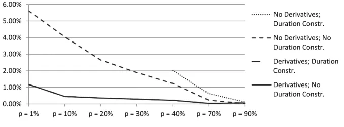
Figure 3 below compares the TE with and without derivatives, and with and without the imposition of the duration constraint when various fractions of the portfolio are invested for the replication.
17
Fig. 3 Tracking error comparison
This figure presents a comparison of the annualized ex-ante TE with and without derivatives, and with and without the duration constraint when various fractions of the portfolio are invested for the replication. Benchmark taken on 3 October 2011.
As the figure shows, when the use of derivatives is not allowed, the relaxation of the duration constraint leads to a substantial drop in the TE and a solution of the optimization for lower fractions as well. The use of derivatives with duration constraint leads to a further large reduction of the TE. The relaxation of the duration constraint when derivatives are used does not lead to a discernible drop of the TE. In the figure above, the TE functions with and without duration constraint when derivatives are used almost overlap.
6. Evolution of the Tracking Error
As already confirmed and as expected, the tracking error (TE) is inversely related to the fraction of the portfolio invested for the replication. The subsections below describe the evolution of the TE over the course of our sample period from 1 January 2008 to 3 October 2011. We are interested in the evolution of the TE when the flexibility of using derivatives, such as interest rate futures and bond futures, is not allowed. We consider the evolution of the TE first when the duration constraint is imposed and then when it is relaxed.
6.1. With duration constraint
Figure 4 below presents the evolution of the TE over the sample period for 40%, 70% and 90% invested for the replication. As we have already seen, when the duration constraint is imposed (Problem 2a), the optimization algorithm has no solution for low fractions. The average TE for 40% invested for the replication is 2.09%, for 70% it is 0.59% and for 90% it is 0.13%.
0.00% 1.00% 2.00% 3.00% 4.00% 5.00% 6.00% p = 1% p = 10% p = 20% p = 30% p = 40% p = 70% p = 90% No Derivatives; Duration Constr. No Derivatives; No Duration Constr. Derivatives; Duration Constr. Derivatives; No Duration Constr.
18
Fig. 4 Tracking error with duration constraint
This figure presents the evolution of the annualized ex-ante TE for various fractions of the portfolio invested for the replication with duration constraint. Derivatives are not used. Sample period is 1 January 2008 to 3 October 2011.
6.2. Without duration constraint
As figure 5 below shows, when the duration constraint is relaxed (Problem 2b), the evolution of the TE follows a similar path. The figure shows the evolution of the TE for the same fractions of the portfolio as in figure 4. This time, the average TE for 40% invested for the replication is 1.70%, for 70% it is 0.41% and for 90% it is 0.07%. As expected, the flexibility due to the relaxation of the duration constraint leads to a lower average TE over the course of the sample period.
Fig. 5 Tracking error without duration constraint (Variant 1)
This figure presents the evolution of the annualized ex-ante TE for the same fractions of the portfolio as in figure 4 without duration constraint. Derivatives are not used. Sample period is 1 January 2008 to 3 October 2011.
Figure 6 below is a superset of figure 5, where the evolution of the TE for lower fractions is presented as well. The figure shows that the TE is consistently and distinguishably different for the different
0.00% 0.50% 1.00% 1.50% 2.00% 2.50% 3.00% 3.50% Jan -08 Ap r-08 Ju l-08 Oct-08 Jan -09 Ap r-09 Ju l-09 Oct-09 Jan -10 Apr-10 Ju l-10 Oct-10 Jan -11 Ap r-11 Ju l-11 Oct-11 p = 40% p = 70% p = 90% 0.00% 0.50% 1.00% 1.50% 2.00% 2.50% 3.00% Jan -08 Ap r-08 Ju l-08 Oct-08 Jan -09 Ap r-09 Ju l-09 Oct-09 Jan -10 Ap r-10 Ju l-10 Oct-10 Jan -11 Ap r-11 Ju l-11 Oct-11 p = 40% p = 70% p = 90%
19
fractions over the sample period. On the other hand, the TE for the different fractions follows a broadly similar pattern.
Fig. 6 Tracking error without duration constraint (Variant 2)
This figure presents the evolution of the annualized ex-ante TE for various fractions of the portfolio invested for the replication without duration constraint. Derivatives are not used. Sample period is 1 January 2008 to 3 October 2011.
Table 15 below presents the average TE over the sample period for various fractions of the portfolio invested for the replication when the duration constraint is relaxed.
Table 15 Average tracking error without duration constraint
This table presents the average annualized ex-ante TE for various fractions of the portfolio invested for the replication without duration constraint. Derivatives are not used. Sample period is 1 January 2008 to 3 October 2011.
Fraction of portfolio Average annualized ex-ante TE
= 1% 6.00% = 10% 4.62% = 20% 3.29% = 30% 2.42% = 40% 1.70% = 70% 0.41% = 90% 0.07%
Figures 4, 5 and 6 raise the question of why the TE has this particular evolution over the sample period. As is evident from the figures, the TE rises in 2008 and decreases in 2009 only to rise again slightly at the end of the sample period. There could be two possible explanations to this pattern.
0.00% 1.00% 2.00% 3.00% 4.00% 5.00% 6.00% 7.00% 8.00% 9.00% Jan -08 Ap r-08 Ju l-08 Oc t-08 Jan -09 Ap r-09 Ju l-09 Oct-09 Jan -10 Ap r-10 Ju l-10 Oct-10 Jan -11 Ap r-11 Ju l-11 Oct-11 p = 1% p = 10% p = 20% p = 30% p = 40% p = 70% p = 90%
20
The objective function in the minimization problems shows that the tracking error is a function of the key rate duration by maturity bucket and of the covariance matrix. So the first explanation has to do with the structure of the benchmark. A change in the structure of the benchmark over the sample period could translate into a change in the size of the TE.
The other possible explanation has to do with a change in the covariance matrix induced by the financial crisis in 2008-2009. In a crisis environment correlations normally rise – this is the case of the USGG daily spot rates which are used for the calculation of the covariance matrix. Moreover, during the 2008-2009 period the rates exhibit increased volatility as well.
Fig. 7 Average covariance of the USGG daily spot rates
This figure presents the evolution of the average covariance of the USGG daily spot rates for a sample period from 1 January 2008 to 3 October 2011. The covariances for each date are calculated with a one-year lag, using the preceding 260 daily rate changes.
The covariance is positively related to both the correlation and the standard deviations. In consequence, figure 7 above shows that there is a large increase in the average covariance of the USGG rates in the 2008-2009 period. We can also see a slight increase in the average covariance at the end of the sample period as well. By comparing figure 2 with figure 7, we can see that the average covariance is far more volatile than the key rate duration by maturity bucket. Based on this remark, we can conclude that the main driver for the evolution of the TE is not the evolution of the benchmark structure (the weighted key rate duration by maturity bucket) but the evolution of the covariances of the different rates
6.3. Principal component analysis
Indeed, the TE in our sample period can be almost perfectly explained by the evolution of the covariance matrix of the USGG daily spot rates. In order to gain further insight into the behavior of the TE, we performed principal component analysis (PCA) – a procedure that applies an orthogonal transformation to a set variables to produce a set of linearly uncorrelated variables called principal components. The transformation is defined so that the first principal component explains the largest proportion of the variance, and so on. In our case, PCA consists of an eigenvalue decomposition of
0.000 0.002 0.004 0.006 0.008 0.010 Jan -08 Ap r-08 Ju l-08 Oct-08 Jan -09 Ap r-09 Ju l-09 Oct-09 Jan -10 Ap r-10 Ju l-10 Oct-10 Jan -11 Ap r-11 Ju l-11 Oct-11 Average Covariance
21
the covariance matrix. Since we have a positive definite matrix of the yields, all our eigenvalues are positive. The importance of the th principal component, the eigenvector , is determined by the size of its eigenvalue . The explanatory power of , i.e. the proportion of the variance explained by the th principal component, is calculated as ∑ , where is taken over all eigenvalues. In an attempt to model the term structure of interest rates, studies have found that using the first three principal components of the covariance or correlation matrix already accounts for 95% to 99% of the variability. These results were first observed by Steely (1960) and Litterman and Scheinkman (1961). The first principal component is usually flat, i.e. it has the same sign across the term structure. The second principal component has opposite signs at the two extremes of the maturity spectrum and only one sign change in between. The third principal component has the same sign at the two extremes and two sign changes in between. These three principal components are generally interpreted in the literature as the level, slope and curvature of the term structure.
Several studies have addressed the mathematical interpretation of the level-slope-curvature effect. Forzani and Tolmasky (2003) observe the level-slope-curvature effect for high correlations using exponentially decaying correlation function. Lord and Pelsser (2005) use the theory of total positivity to define sufficient conditions for the level-slope-curvature effect. Provided that correlations are positive, Perron’s theorem stipulates that the first principal component will have no sign changes. Slight alterations of several theorems by Gantmacher and Krein provide sufficient conditions for level, slope and curvature. Roughly speaking, according to these conditions the correlation curves should be flatter and less curved for larger tenors, and steeper and more curved for shorter tenors. Figure 8 below superimposes the evolution of the TE over the principal components’ explanatory power. The comparison with the TE is not obvious – they are different measures. The only thing that we can say is that the ratio of the variance explained by the different principal components changes over time with the TE. The first principal component explains roughly between 84% and 94% of the yields’ variability. Adding the second and third principal component boosts the explanatory power to 96% - 99%. In the worst case, the first principal component still explains 84% of the total variability. This seems to be an excellent score. We should say, however, that in periods of high stress it is important to consider the second principal component to obtain a ratio for the explained variance of around 95%.
22
Fig. 8 Explanatory power of the first three principal components vs. the tracking error
This figure presents the evolution of the explanatory power of the first three principal components vs. the evolution tracking error with 40% of the portfolio invested for the replication, without derivatives and without duration constraint, for a sample period from 1 January 2008 to 3 October 2011.
In order to have a proper understanding of the evolution of the principal components, we must first examine the behavior of the yields. Figure 9 below presents the evolution of the USGG spot rates from 1 January 2007 to 3 October 2011. Our sample period starts in 2008. However, since the covariances are calculated with a one-year lag, the coverage in the figure starts in 2007.
Fig. 9 The USGG daily spot rates
This figure presents the evolution of the USGG daily spot rates from 1 January 2007 to 3 October 2011, i.e. starting one year before the beginning of the sample period.
In the beginning of 2007, the rates are very similar across the maturity spectrum – hovering around 4% to 5%. Afterwards, the short-term rates drop to very low levels (below 1%). The medium and long-term rates also drop but not nearly as much – they remain in the region of 1% to 5%. Hence,
0.50% 1.00% 1.50% 2.00% 2.50% 80% 85% 90% 95% 100% Jan -08 Ap r-08 Ju l-08 Oct-08 Jan -09 Ap r-09 Ju l-09 Oct-09 Jan -10 Ap r-10 Ju l-10 Oct-10 Jan -11 Ap r-11 Ju l-11 Oct-11 First PC First two PC's First three PC's TE 0.00% 1.00% 2.00% 3.00% 4.00% 5.00% Jan -07 Ap r-07 Ju l-07 Oct-07 Jan -08 Ap r-08 Ju l-08 Oct-08 Jan -09 Ap r-09 Ju l-09 Oct-09 Jan -10 Ap r-10 Ju l-10 Oct-10 Jan -11 Ap r-11 Ju l-11 Oct-11 USGG1Y USGG2YR USGG3YR USGG5YR USGG7YR USGG10YR USGG30YR
23
their daily variations become far more important compared to those of the shorter-term rates. Moreover, in figure 9 we can see the increased variability of the yields from mid-2007 to mid-2009 – a period that includes the fall of Lehman Brothers and the credit crunch. Figure 8 shows that the TE picks up this effect through the covariance matrix roughly six months to one year later.
Fig. 10 The first three principal components
This figure presents the evolution in increasingly darker shades of gray of the first three principal components of the covariance matrix for each month for a sample period from 1 January 2008 to 3 October 2011.
Panel A: First principal component
Panel B: Second principal component
Panel C: Third principal component 0.00 0.10 0.20 0.30 0.40 0.50
[0Y-1.5Y] [1.5Y-2.5Y] [2.5Y-4Y] [4Y-6Y] [6Y-8.5Y] [8.5Y-20Y] [+20Y]
-0.90 -0.60 -0.30 0.00 0.30 0.60 0.90
[0Y-1.5Y] [1.5Y-2.5Y] [2.5Y-4Y] [4Y-6Y] [6Y-8.5Y] [8.5Y-20Y] [+20Y]
-0.60 -0.30 0.00 0.30 0.60 0.90
24
Figure 10 above presents the evolution in increasingly darker shades of gray of the first three principal components, or eigenvectors, from 1 January 2008 to 3 October 2011. Noticeably, the entries of all three eigenvectors change with time shifting towards longer-term maturities. Panel A of figure 10 shows that the part of the variability explained by the long-term maturities has become more important with time. Indeed, the evolution of the first principal component shows that the proportion of the variability explained by the longer-term maturities has grown. This is obvious when we look at figure 9. Whereas in 2007 all rates have more or less similar variability, since the beginning of 2009 the variability of each rate is roughly proportional to its maturity.
The second principal component is generally interpreted as a slope or trend of the yield curve. Panel B in figure 10 thus shows a steepening of the yield curve. As figure 9 shows, the rate differentials have widened significantly over the sample period. Figure 11 below explicitly shows the increasing differential between the one-year and the 30-year rate. The third principal component is generally interpreted as a curvature, twist or butterfly. The variability explained by this eigenvector is so small that its effect is negligible in our case. On average it explains only 2.26% of the variability in the covariance matrix.
Fig. 11 Yield differential between the one-year and the 30-year yield
This figure presents the evolution of the differential between the one-year and the 30-year yield from 1 January 2007 to 3 October 2011.
Figure 9 shows why the explanatory power of the first principal component is reduced while that of the second principal component is increased during the period of high stress around 2009. During this time the variability of the yields per se was not the only explanatory factor. We can observe the large increase in the yield differentials approximately one year to six months earlier, which is captured by the increased explanatory power of the second principal component. In conclusion, we can observe that the variability, or in other words the volatility, of the yields and their increasing differentials explain around 95% of the covariance, which in turn is the main driver of the size of the TE. -1.00% 0.00% 1.00% 2.00% 3.00% 4.00% 5.00% Jan -07 Ap r-07 Ju l-07 Oct-07 Jan -08 Ap r-08 Ju l-08 Oct-08 Jan -09 Ap r-09 Ju l-09 Oct-09 Jan -10 Ap r-10 Ju l-10 Oct-10 Jan -11 Ap r-11 Ju l-11 Oct-11 USGG30YR -USGG1YR
25
7. Concluding Remarks
This article offered a generic method for the replication of a bond benchmark with the flexibility of using derivatives (interest rate futures and bond futures) or not. The crux of our methodology is the minimization of the tracking error (TE), i.e. the variation of the fraction of the portfolio invested for the replication versus full investment. We should stress again that we approach the TE on an ex-ante basis, as an ex-post calculation would require knowledge of the realized performance of the benchmark and our fictitious portfolios. The rolling analysis provides some major insights into the evolution of the TE. Namely, it is related to the prevailing economic conditions. The principal component analysis indicates that changes in the variability of the spot rates used in the calculation of the covariance matrix and their widening differentials are the main determinants of the TE. More importantly, however, the results we obtain during our sample period from 1 January 2008 to 3 October 2011 suggest that reasonably low values of the TE can be achieved even without using derivatives for the replication. The size of the TE changes considerably over the sample period. Nevertheless, on average, when the duration constraint is imposed, for 40% of the portfolio invested for the replication the annualized ex-ante TE is 2.09%, for 70% it is 0.59% and for 90% it is 0.13%. When the duration constraint is relaxed, the TE is further reduced. For 40% it becomes 1.70%, for 70% it becomes 0.41% and for 90% it becomes 0.07%. Therefore, for 70% to 90% invested for the replication, the performance is reasonably close.
Our methodology therefore goes one step further than previous studies having tackled the bond index replication problem mainly through the use of liquid derivatives. Here we provide a framework which is very appropriate when the use of derivatives is prohibited. With the approach developed here, we can benefit from replicating a traditional investment in a bond index with a fraction of the portfolio according to our risk appetite. The rest of the portfolio would allow us to gain exposure to riskier strategies with potentially higher return. Our methodology thus offers a generic and intuitive yet robust approach to derivative-free bond index replication.
Acknowledgements
We would like to thank the editorial team of FMPM. We would also like to thank the anonymous referee for providing useful comments and suggestions that helped us improve and refine our work.
Disclaimer: The views expressed in this article are the sole responsibility of the authors and do not necessarily reflect those of Pictet Asset Management or Tages Capital LLP. Any remaining errors or shortcomings are the authors’ responsibility.
26
8. References
Cheng, P.L.: Optimum bond portfolio selection. Manag. Sci. 8(4), 490–499 (1962)
Cox, J.C., Ingersoll, J., Ross, S.: A theory of the term structure of interest rates. Econom. 53(2), 385– 407 (1985)
Dynkin, L., Hyman, J., Lindner, P.: Hedging and replication of fixed-income portfolios. J. Fixed Income 11(4), 43-63 (2002)
Dynkin, L., Gould, A., Konstantinovsky, V.: Replicating bond indices with liquid derivatives. J. Fixed Income 15(4), 7-19 (2006)
Elton, E.J., Gruber, M., Brown, S., Goetzmann, W.: Modern Portfolio Theory and Investment Analysis, 6th ed. Wiley, New York (2003)
Forzani, L., Tolmasky., C.: A family of models explaining the level-slope-curvature effect. Int. J. Theor. Appl. Financ. 6(3), 239–255 (2003)
Higham, N.J.: Computing a nearest symmetric positive semidefinite matrix. Linear Algebr. Appl. 103(6), 103-118 (1988)
Korn, O., Koziol, C.: Bond portfolio optimization: A risk-return approach. J. Fixed Income 15(4), 48-60 (2006)
Litterman, R., Scheinkman, J.: Common factors affecting bond returns. J. Fixed Income 1(1), 54–61 (1991)
Lord, R., Pelsser, A.: Level-slope-curvature – Fact or artifact? Tinbergen Institute discussion paper TI 2005-083/2 (2005)
Markowitz, H.M.: Portfolio selection. J. Financ. 7(1), 77–91 (1952)
Puhle, M.: Bond Portfolio Optimization. Springer-Verlag, Berlin, Heidelberg (2008)
Steely, J.M.: Modelling the dynamics of the term structure of interest rates. Econ. Soc. Rev. 21(4), 337–361 (1990)
Vasicek, O.: An equilibrium characterization of the term structure. J. Financ. Econ. 5(2), 177–188 (1977)
Wilhelm, J.: Fristigkeitsstruktur und Zinsänderungsrisiken - Vorüberlegungen zu einer Markowitz-Theorie des Bond-Portfolio-Managements. Z. Betriebswirtsch. Forsch. 44, 209-246 (1992)
Iliya Markov is a research assistant at Haute Ecole de Gestion, Geneva. He has an MSc in Operational Research with Finance from the University of Edinburgh and a BA in Mathematics and Economics from the American University in Bulgaria. In recent years, Iliya has published several book chapters and articles. He is a recipient of several awards and distinctions including an Outstanding Achievement in Mathematics at the American University in Bulgaria.
Rodrigue Oeuvray currently works as a senior investment risk manager in the fixed income department of Pictet Asset Management in Geneva. Before joining Pictet, he served as a senior
27
financial engineer and as a statistical consultant at Insightful in Zurich. Rodrigue holds an MSc in Mathematical Engineering and a PhD from the Swiss Institute of Technology of Lausanne (Ecole Polytechnique Fédérale de Lausanne) in Switzerland. He is also a Financial Risk Manager (FRM - GARP) and an analyst in alternative investments (CAIA). He has also passed the Wilmott certificate in quantitative finance.
Nils Stéphane Tuchschmid is a partner and head of directional strategies at Tages Group. Before joining Tages, he was a professor of banking and finance at the Haute Ecole de Gestion, Geneva. Previously, Nils served as co-head of Alternative Funds Advisory at UBS within Alternative and Quantitative Investment and, prior to joining UBS, he served as head of multi-manager portfolios at Credit Suisse within Funds & Alternative Solutions. Nils was head of quantitative research and alternative investments at Banque Cantonale Vaudoise and a professor of finance at HEC Lausanne University. He earned an M.D. master’s degree in Economics from the University of Geneva and a PhD in Economics, summa cum laude, from the University of Geneva.