Simultaneous Allocation of Bundled Goods Through Auctions: Assessing the Case for Joint Bidding

Texte intégral

(1)2013s-37. Simultaneous Allocation of Bundled Goods Through Auctions: Assessing the Case for Joint Bidding Daniel Rondeau, Pascal Courty, Maurice Doyon. Série Scientifique Scientific Series. Montréal Septembre 2013. © 2013 Daniel Rondeau, Pascal Courty, Maurice Doyon. Tous droits réservés. All rights reserved. Reproduction partielle permise avec citation du document source, incluant la notice ©. Short sections may be quoted without explicit permission, if full credit, including © notice, is given to the source..

(2) CIRANO Le CIRANO est un organisme sans but lucratif constitué en vertu de la Loi des compagnies du Québec. Le financement de son infrastructure et de ses activités de recherche provient des cotisations de ses organisations-membres, d’une subvention d’infrastructure du Ministère du Développement économique et régional et de la Recherche, de même que des subventions et mandats obtenus par ses équipes de recherche. CIRANO is a private non-profit organization incorporated under the Québec Companies Act. Its infrastructure and research activities are funded through fees paid by member organizations, an infrastructure grant from the Ministère du Développement économique et régional et de la Recherche, and grants and research mandates obtained by its research teams. Les partenaires du CIRANO Partenaire majeur Ministère de l'Enseignement supérieur, de la Recherche, de la Science et de la Technologie Partenaires corporatifs Autorité des marchés financiers Banque de développement du Canada Banque du Canada Banque Laurentienne du Canada Banque Nationale du Canada Banque Scotia Bell Canada BMO Groupe financier Caisse de dépôt et placement du Québec Fédération des caisses Desjardins du Québec Financière Sun Life, Québec Gaz Métro Hydro-Québec Industrie Canada Investissements PSP Ministère des Finances et de l’Économie Power Corporation du Canada Rio Tinto Alcan State Street Global Advisors Transat A.T. Ville de Montréal Partenaires universitaires École Polytechnique de Montréal École de technologie supérieure (ÉTS) HEC Montréal Institut national de la recherche scientifique (INRS) McGill University Université Concordia Université de Montréal Université de Sherbrooke Université du Québec Université du Québec à Montréal Université Laval Le CIRANO collabore avec de nombreux centres et chaires de recherche universitaires dont on peut consulter la liste sur son site web. Les cahiers de la série scientifique (CS) visent à rendre accessibles des résultats de recherche effectuée au CIRANO afin de susciter échanges et commentaires. Ces cahiers sont écrits dans le style des publications scientifiques. Les idées et les opinions émises sont sous l’unique responsabilité des auteurs et ne représentent pas nécessairement les positions du CIRANO ou de ses partenaires. This paper presents research carried out at CIRANO and aims at encouraging discussion and comment. The observations and viewpoints expressed are the sole responsibility of the authors. They do not necessarily represent positions of CIRANO or its partners.. ISSN 2292-0838 Partenaire. financier.

(3) Simultaneous Allocation of Bundled Goods Through * Auctions: Assessing the Case for Joint Bidding Daniel Rondeau †, Pascal Courty ‡, Maurice Doyon§. Résumé/abstract We use the experimental method to study the costs and benefits of allowing joint bidding in simultaneous multi-unit first price sealed bid auctions for bundled goods. The research has immediate applications to the sale of public forest stands that arbor a mixture of species. Joint bidding and communication raise the prospect of higher allocative efficiency, but also of collusive bidding through a reduction in the number of bidders and a greater scope for the formation of bidding rings. However, we find that allowing joint bidding has a significant positive impact on efficiency and reduces collusion significantly. We also explore the robustness of the results to characteristics of the auction environment that are relevant to timber auctions. Mots clés/Keywords : Timber auctions; forest industry; joint bidding; bidding rings; collusion; simultaneous auction; starting price; two bidder rule. Codes JEL : Q23 (Forestry); Q28 (Government Policy); D44 (Auctions); D47 (Market Design). *. This research was sponsored by the Ministère des Ressources Naturelles du Québec. The analysis and opinions presented in this paper are exclusively those of the authors and in no way those of the sponsor. Errors remain our sole responsibility. We are grateful for the excellent research assistance provided by Samuel Lee and Alison Watt. † Corresponding author. CIRANO and Department of Economics, University of Victoria, PO Box 1700 Stn CSC, Victoria, BC Canada, V8W 2Y2, rondeau@uvic.ca; tel.:+1-250-472-4423; fax: +1-250-721-6214. ‡ Department of Economics, University of Victoria, Canada, Department of Economics, University of Victoria, PO Box 1700 Stn CSC, Victoria, BC Canada, V8W 2Y2. § CIRANO and Department of Agricultural Economics and Consumer Science, Laval University, 2425, rue de l'Agriculture, Québec, Qc, Canada, G1V 0A6.

(4) 1. Introduction First price sealed bid auctions are used to allocate the rights to harvest publicly owned forests in many jurisdictions (e.g. U.S. National Forest Service; British Columbia, France; see for instance Athey and Levin 2001; Athey et al. 2004; Baldwyn et al. 1997; Li and Perrigne 2003; Mead 1967; Paarsch 1991). Recent adopters of auction mechanisms aim to modernize their forest tenure systems in both North America (the province of Quebec introduced an auction system in 2012) and in Eastern Europe (e.g. Romania; Saphores et al. 2007). Unfortunately, the economic realities of forest harvesting and timber processing often make forest sector markets less than ideally competitive. Lumber and paper production most often require a significant scale and the legacy of forest tenure systems that ensured extensive supply of fiber over long time horizons to few firms has translated today in a small number of forest users thinly spread over a large territory. Thus, the transportation costs associated with a given stand can vary substantially across potential buyers, often leaving local firms with a considerable competitive advantage. Compounding these problems is the ability of firms in small markets to collude. The potential for collusion in sealed bid auctions conducted in small markets has been recognized for some time. Isaac and Walker (1985) showed that participants are often able to form stable bidding rings to reduce competition and prices. Sherstyuk (1999) and Kwasnica (2000) extend this result to an environment particularly relevant to this research, where multiple units are sold simultaneously. In this paper, we put in place a policy relevant experimental timber auction environment that replicates the main features of Quebec’s new forest auction design for bundled goods. We measure the impact of allowing joint bidding on bidding behavior, revenue and efficiency. We also investigate the robustness of the results to auction characteristics that matter in an application to timber. The basic set up is a multiple unit first price sealed bid auction for bundled goods. Six participants are presented a total of eight lots each round. Participants, however, cannot bid on all lots. Each lot can be offered to either three or all six players. In most treatments, all six bidders have a “soft” limit on their capacity to process the lots they win. This is implemented by imposing a cost on bidders who win more than two lots, reflecting the absence of a dependable resell market. Perhaps the most salient feature of the Quebec auctions is the ability of bidders to join forces and bid in teams. Joint bidding is allowed in recognition of the fact that most forest stands in Quebec (and indeed in many other jurisdictions) are composed of two or more distinct tree species destined to specific usage and types of mills (e.g. lumber for some species and pulp and paper for others; softwood and hardwood). Thus, it is often the case that a potential buyer only values one of the species growing on a given lot. Even if a stand is entirely composed of hardwood species,.

(5) specialized mills often require one type only, leaving them with little or no value for the other wood available on a stand offered at auction. De facto, each lot is a bundle of multiple goods. Formal joint bidding allows for efficiency gains to be realized at the auction stage. However, doing so may also reduce competition. Another drawback is that allowing the formation of consortia inevitably requires legalizing communication between firms, making it easier for firms to collude in other ways.1 The net impact of allowing joint bidding on revenue is therefore ambiguous. Within this general framework, we study the effect of allowing joint bidding on bidding behavior and market outcomes. Because we wish to isolate the impact of joint bidding, we allow communication both when joint bidding is allowed and when it isn’t. Results show that when joint bids are allowed, bidders focus their efforts towards securing efficiency-enhancing joint bids. As a result, bidders who form joint bids have typically higher valuation and make higher bids. Solo bidders (the bidders who do not make joint bids) bid a higher fraction of their valuation when joint bids are allowed. The main concern with joint bidding is that it may increase collusion. Collusion can take place through a deliberate reduction in the number of bidders. It may also facilitate the formation of effective bidding rings whereby bidders agree not to compete against one another, and allocate the lots available among themselves. It is usually not possible to identify collusive biding precisely. However, the auction design implemented in this research produces a fairly reliable ‘smoking gun’ sign that groups of bidders have agreed to split the market. Using this measure, we find that the ability of bidders to communicate when they cannot submit joint bids results in substantial market splitting and lower prices. Such collusive behavior is much less present when joint bids are allowed. The net result of allowing joint bids is therefore an increase in both revenue and efficiency despite the fact that doing so reduces the number of bidders on a lot. We are also interested in the role of other auction rules and characteristics of the auction environment that are relevant to an application to timber in Quebec and elsewhere. Specifically, we discuss in a robustness section the impact of: i) Imposing that a minimum of two bids must have been received for the lot to be awarded (the “two bidder rule”). The two bidder rule does not appear to have a direct effect on collusive agreements. Overall, the rule increases auction revenue without affecting efficiency. Most importantly, the two bidder rule opens a window to observe the. Although engaging in market splitting or other forms of collusive strategies is still prohibited by Canadian competition laws (Canada Competition Act 1985), proving collusive behavior would be extremely difficult when communication between competitors is permitted for the purpose of forming joint bids. 1. 2.

(6) presence of collusive bidding because it forces bidding rings to submit low sham bids that can leave a trace in the data. ii) The effect of introducing two players who, contrary to others, do not have a capacity constraint (they do not pay a penalty for winning more than two lots). The presence of a soft capacity constraint decreases average bids, but not the average winning bids. iii) Doubling the number of lots offered in order to study the effect of offering “excess supply”. Excess supply leads to rampant collusive bidding and significantly decreases both bids and revenue. Overall, fears that allowing joint bidding might lead to both collusion and lower bids due to decreased competition did not materialize in the experiment. Acknowledging that an experiment is not the same as a live auction, the results have implications for auctions and market design but also addresses one of the long standing and unresolved questions surrounding the formation of joint ventures in general. While forming complementary partnerships can increase overall firm productivity or the rate of innovation, it also reduces competition in the relevant market. The net effect of joint bidding or R&D ventures is therefore ambiguous (d'Aspremon and Jacquemin 1988; Farrell and Shapiro 1990 and Kamien et al. 1992). There is very little evidence on the efficiency effect of R&D ventures (Cassiman andVeugelers 2002; Gugler and Siebert 2007 and Duso et al. 2010). The only experimental evidence we are aware of (Suetens 2005 and 2008) does not address the efficiency trade-offs between complementary matching and collusive bidding. Our results provide one example where allowing joint bidding produced substantial efficiency gains and increased revenue, despite the fact that with joint bidding comes greater opportunities to collude and divide the market,. Taken together, the results tend to suggest that it is possible to design a sufficiently rich set of rules to deter wholesale collusion in thin markets. Our new approach to identify collusion contributes to the large literature on collusion in auction (Isaac and Walker 1985; Hendricks and Porter 1989; Porter and Zona 1993; Kwasnica 2000 and Gupta 2001 and 2002) and specific applications to timber (Baldwin et al. 1997 and Saphores et al. 2007). The two bidder rule can help auction designers interpret bidding behavior and detect collusion. In the next section, we proceed directly to a description of the experimental design and of the various auction characteristics tested in this research. Once this is done, we explore some of the implications of allowing joint bidding and present the main results. We then discuss the robustness of these results in light of alternative rules and environmental conditions. We conclude with a general discussion of our findings.. 3.

(7) 2. A Policy-Based Experimental Design In March and April 2012, 150 students from the University of Victoria (Canada) participated in experimental auctions in groups of six. Participants were inexperienced subjects, primarily in business and economics (third or fourth year undergraduate or graduate students). Each group participated in a total of 12 auctions: 2 practice auctions without real payoffs and 10 paying auctions. Sessions lasted on average two hours and twenty minutes and carried unusually high payoffs for most economics experiments. Subjects received an average (confidential) cash payment of CA$82 for their efforts (ranging between CA$20 and CA$155), with those earnings based entirely on the profits they realized in the auctions. A session began with oral instructions supported by a PowerPoint presentation. As part of the instructions, a full round of trading was completed in order to familiarize participants with the computer interface and computation of results. Each group of students was assigned to one of five treatments of ten computer-mediated auctions deployed on ZTree (Fischbacher, 2007). Communication between participants was allowed for up to 3.5 minutes per auction. At the beginning of an auction, each participant was presented with a screen reproduced as Figure 1. The screen contains several elements of information. In the center, each subject sees between 2 and 8 squares of information. Each square is a separate lot (from A to H) on which the participant can bid. A lot is meant to represent a physical track of forest for which the seller wishes to auction the harvesting rights. The total private value of a lot to the subject is the sum of two separate good values representing two distinct tree species. Each good value is an integer drawn independently from the set {1,2,..,80} with equal probability, to mimic a uniform distribution. On the right side of the screen, a table made public that either three or six players could bid on each lot and who they were. Two other critical pieces of information appear on the top left corner of the screen. First is a “penalty per lot in excess of two”. The other is the “starting price” of 86. In our design, as in real auctions, subjects could bid on as many lots as the number they were offered. If lots were perfectly independent from one another, players should bid on every lot presented to them. However, this would have been a major departure from the policy context for timber auctions. In reality, mills have a fixed capacity and a regulatory obligation to harvest lots within a fixed time limit. Thus, winning “too many” lots at auction imposes additional transactions costs and exposes the firm to risks of having to harvest but be unable to recoup their purchase price on a thin informal secondary market. To simulate this soft capacity constraint, a penalty of 10 ECU2 per good in excess of four was imposed on subjects who purchased more than four goods. 2. ECU is an experimental currency unit, which is converted in Canadian $ at the end of the experiment.. 4.

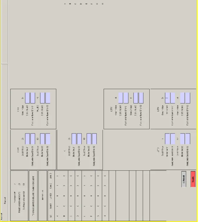
(8) (corresponding to two full lots) in a given auction. For example, a subject who wins three full lots and one good in a joint bid (a total of 7 goods) would get a penalty of 30 deducted from his profits. Figure 1: Participant Information and Bidding Screen. 5.

(9) The final central feature of the auction design is the use of a reserve price with a conditional allocation rule. Specifically, the allocation rule for the auction on each lot is constructed around an unannounced random reserve price drawn from the unannounced uniform integer distribution with support {51, 52,..,60}, and the public starting price of 86 ECU. The reserve price is the absolute minimum at which the seller is willing to sell the lot. However, the two bidder rule states that if the highest bid falls between the reserve and starting prices, the allocation will take place only if at least two bids were received for the lot. The two bidder rule is meant to mimic Quebec’s tendering law which has similar requirements. It is thought to increase the cost of collusion attempts, but also, in combination with the reserve and starting price, to increase the price in thin markets. As they consulted their information screen, participants had the opportunity to copy key data onto a sheet of paper that generically reproduced the basic computer screen (i.e. boxes for all eight possible lots but without any private values printed). They could then stand up and mingle in different parts of the lab in quiet discussions to explore joint bidding opportunities with others. The sheet of paper was added to the design to prevent players from credibly revealing their private values to others and experimenters strictly enforced that all computer displays be turned off during the communication period. Subjects were actively discouraged from showing their sheet of paper to one another but the rule was difficult to enforce perfectly. Thus we also suggested during the instructions that participants did not have to copy exact values (e.g. they could copy their real value minus a constant for instance) and could therefore be deceived if shown another participant’s sheet. This was done to further reduce the credibility of information about values that was divulged in conversations, since such information cannot be verified in real auctions. At the conclusion of each communication period, participants were asked to return to their workstation and enter their bids. Fields left blank were recorded as no bids (zeros in the data) and had no chance of winning. In the case of joint bids, the two bids for Good 1(by one player) and Good 2 (by the other) had to be entered by both players. These were binding agreements and bids could not be accepted by the computer system until the participants who agreed to bid jointly entered identical bidding amounts on their respective data entry screens. Absent a perfect match of these four data fields, the server returned an error message indicating a mismatch.3 Once all bids were acceptable, the server allocated lots to the highest bid above zero (based on the sum of the bids for Goods 1 and 2) and returned the results to players. At the conclusion of an auction, all players received a table indicating the lots they won and their profits, as well as whether or not each of the Experimenters monitored the data entry from the back of the lab and helped reconcile those errors. This prevented subjects from having to stand up at this stage of the round and possibly glance at other player’s information. It also ensured that players could not reveal that a lot was being subject to a joint bid. 3. 6.

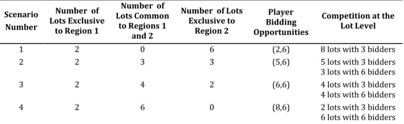
(10) other lots sold. Thus, the bid data from subjects remained private and no feedback other than "sold" or "did not sell" was given to a subject who did not win the lot. Each auction implements one of four configurations of the lots that players can bid on (information displayed on the table on right hand side of Figure 1). These four configurations presented in Table 1 are meant to artificially represent different regional and inter-regional competitiveness scenarios.4 Competitiveness is constant in region 1 (Column 2) but varies for interregional lots (Column 3) and in region 2(Colunm4). Although there are 8 lots and 6 bidders in each scenario, competitiveness varies greatly at the lot level (Column 6). Participants were reassigned at random to region 1 and region 2 with each new auction. As such participants did not have a perfect ability to form stable coalitions since they could not count on the next offering to assemble the same subgroup of players. Though the reality in the field could allow more stable coalitions, it is also true that outside firms have been observed bidding where they would not be expected to do so regularly, thus making effective coalition formation more difficult. Table 1: “Regional Distributions” of Auctioned Lots Scenario Number. Number of Lots Exclusive to Region 1. Number of Lots Common to Regions 1 and 2. Number of Lots Exclusive to Region 2. Player Bidding Opportunities. Competition at the Lot Level. 1 2. 2 2. 0 3. 6 3. (2,6) (5,6). 3. 2. 4. 2. (6,6). 4. 2. 6. 0. (8,6). 8 lots with 3 bidders 5 lots with 3 bidders 3 lots with 6 bidders 4 lots with 3 bidders 4 lots with 6 bidders 2 lots with 3 bidders 6 lots with 6 bidders. Note: The first (second) number in column 5 denote the number of lots that the three bidders in region 1 (2) can bid on. The array of regional distribution scenarios replicates the decentralized timber management regime implemented in many jurisdictions, including Canadian provinces and in One can think of the regional distributions as various spatial representations of the lots offered at auction with 3 bidders located in each of two regions. Lots offered can generate an interest from bidders in either one of the regions, or in both (i.e. when they are located near the edge or between the two regions). For instance, scenario 1 has three bidders vying only for 2 lots located in Region 1, while three bidders compete for 6 lots offered in Region 2. No lot is offered that is of interest simultaneously to bidders in both regions. If we look at this auction from the perspective of competition for lots (the last column), we observe that all eight lots offered have 3 potential bidders. At the other extreme, 2 lots are offered exclusively to the three bidders of Region 1 and the other six are of interest to everyone. As a result, the two lots of region 1 can be bid on by 3 players, while the six lots of the inter region can be bid on by all six players. 4. 7.

(11) auctions conducted by the U.S. National Forest Service. The four scenarios reflect heterogeneity in the degree of competitiveness that is due to a geographically diverse offering. While such scenarios help us make the design more policy relevant, they also introduce data limitations. The variation in the offering across the four scenarios inevitably modifies both the menu of lots that individuals can bid on and the degree of competition for the lots in ways that cannot readily be disentangled because of the systematic correlations that exists between these two variables. For this reason and others (e.g. endogenous joint bidding decisions, discontinuous penalties), the data is ill-suited to a fine analysis of bidding strategies at the individual level. Rather, it is built to gain an overall understanding of the effects of the various treatments and to analyze whether the treatments perform differently when deployed under different regional configuration scenarios. As such, the regional configurations can be viewed as an enhanced stress-test for the auction rules and environmental conditions of each treatment. All the analysis is conducted by comparing moments of distributions across all auctions in a given regional distribution and across regional distributions. This is made possible by the fact that for all sessions, each regional configuration was played once (in random order) in the first four rounds, and once again in random order in rounds 5 to 8. Finally, scenarios 1 and 3 were played again in a random order in rounds 9 and 10. This keeps constant across all groups the number of repetitions of each scenario, the total number of lots offered to individuals, and the overall level of competition for lots. The randomization of each scenario’s order of appearance should eliminate possible order effects. However, given the relatively small number of sessions over which we randomized, we chose to force each scenario to appear once in the first and second groups of four auctions in order to ensure that all groups faced all possible scenarios in the early part of their experiment. The analysis we perform, therefore, does not discuss the variations in regional scenarios other than in the robustness section where we show that the aggregate results hold when we look at the four regional distributions separately. We conducted two main treatments to study the effect of joint bidding and three robustness treatments. The base treatment is the joint bid treatment [T0]. It corresponds most closely to the field conditions envisioned by the agency responsible for the management and sale of Quebec’s public forests. All other treatments modify a single design component from [T0] and should be compared against it: Joint Bid Treatment [T0]. Complete package of auction rules: (a) Eight lots are offered; (b) Joint bidding is permitted; (c) A penalty of 10 experimental currency units is billed for each good won in excess of four goods; (d) The two bidder rule applies. No Joint Bid Treatment [T1]. Joint bidding is not allowed. 8.

(12) Robustness Treatment [R1]: No Two-Bidder Rule. Lots are allocated to the highest bid greater than the random reserve price irrespective of the total number of bids. Robustness Treatment [R2]: Excess Supply. 16 lots rather than 8 are offered in each auction and these sessions allow for 6.5 minutes of communication instead of 3.5. We will compare R2 both with T0 and to another treatment identical to T0 but with 6.5 minutes session length. In doing so, we can separately measure the impact of excess supply. Robustness Treatment [R3]: Dominant Players. Two of the six players have unlimited capacity and therefore do not face a penalty if they purchase more than 2 lots (4 goods). 3. Observations on Joint Bidding Allowing joint bidding may change the auction outcomes through multiple channels. The experimental design allows players to interact, exchange information, and make both explicit joint bidding agreement and implicit collusive agreements. Unstructured interactions change bidder’s information sets and influence bidding in ways that are difficult to capture with simple models. While the complex set of rules implemented in our experiments make the derivation of formal equilibrium bidding predictions impossible, we make, in this section, general remarks on the impact of allowing joint bidding. 3.1. Efficiency Effect: Value Distributions. As we alluded to earlier, allowing joint bids could result in substantial efficiency gains by allowing two potential bidders to combine their high values for the two species growing on a lot. Here, we illustrate for our experiment the underlying distributions of value that single and joint bidders bring to an auction. To keep the focus on bidding strategies, we assume that joint bidders randomly match. In our experiment, the private value of the lot to player i is the sum Vi  vi1  vi 2 where each of. vi1 and vi 2 is an iid random variable drawn from the interval [vmin, vmax]=[1,80]. In what follows, we drop the player index i without loss of generality. With each of v1 and v2 is a uniformly distributed variable, the sum V  v1  v2 takes on a triangular distribution with cumulative distribution function (CDF) of the form. 9.

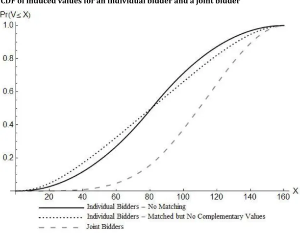
(13) 0  2  ( x  2vmin )  2(vmax  vmin ) 2 Pr(V  x)  F  x    2 1  (2vmax  x)  2(vmax  vmin ) 2  1. x  2vmin 2vmin  x  vmax  vmin. (1). vmax  vmin  x  2vmax 2vmax  x. Now consider two players who meet randomly. If they find that they have complementary values ( vi1  v j1 and vi 2  v j 2 or with both inequalities inverted), they form a joint bid selecting the two high values as the basis of their bid. The resulting distribution of V  v1  v2 for these joint bids is then given by:. 0  4  ( x  2vmin )  6(vmax  vmin ) 4 Pr(V  x)  F  x    2 1   x  2vmax   x  2vmin  (4vmax  6vmin  x)  6(vmax  vmin ) 4  1. x  2vmin 2vmin  x  (vmax  vmin ). (2). (vmax  vmin )  x  2vmax 2vmax  x. This distribution has a mean of 107.33 and a median at 109.27. Figure 2 provides one possible illustration of the advantage that a joint venture holds over a single bidder by plotting the CDF for an individual bidder (solid line), for randomly matched players who have complementary values resulting in a joint bid (long dashes), and for randomly matched pairs who do not have complementary values (short dashes).. 10.

(14) Figure 2: CDF of induced values for an individual bidder and a joint bidder. Of course, one could also construct other distributions. For instance, we could consider a group of three or six players and consider the joint values of the best possible match(es) among those players. Such distributions would stochastically dominate the joint bidder distribution in Figure 2. As such, the joint bidder distribution of Figure 2 should be viewed as the minimum shift in value that can occur when joint bids form endogenously. The joint bidder distribution can also be viewed as a partial representation of the potential efficiency gains from joint bidding. If one assumes that there is no pre or post auction trading of timber resources, and therefore that joint bidding is the only mechanism that allows the best allocation of the two species found on a lot, the rightward shift of the distribution is representative of the higher values brought about by the partnership. It is only a partial indication of potential gains since individuals may form better matches on average than random encounters would. 3.2. Strategic Effects: Decrease in the Number of Bidders. Joint bidding reduces the number of bidders and, everything else equal, bidders bid less aggressively when there are fewer bidders. To illustrate, assume valuations are uniform and i.i.d. on [0,1] in a standard first price sealed bid auction (i.e. one without all of the rules added to our experiment). This distribution of valuations is convenient because (contrary to the triangular 11.

(15) distribution used in the experiment) it delivers a closed form solution of the individual expected profit. In a first price sealed bid auction with n symmetric bidders, a bidder with valuation v earns expected profits. U  v, n .  n  n  1  . n 1. vn. n. .. Now assume that two bidders with identical valuations make a joint bid and split the profits evenly. The number of bids decreases from n to n-1. Clearly, the bidders who do not make a joint bid benefit. However, bidders who make the joint bid also benefit if. U  v, n   U  v, n  1 2 . For n=3 the inequality holds if v<2/3. For n=6, this inequality holds for any v   0,1 . Keeping in mind that the distribution of valuations in the experiment is different, this nonetheless illustrates that reducing competition can be a motivation for joint bidding regardless of the degree of complementarity between bidders' valuations. 3.3. Overall Effect on Bidding Strategies. Let’s return to the point that joint bidders have higher distributions of valuation than individual bidders. By virtue of their stochastically dominant value distribution, joint bidders become dominant bidders relative to individual bidders. Chermonaz (2012) derives the net impact of the two effects discussed above for simpler distributions: (a) a reduction in the number of bidders as discussed above and (b) an asymmetry in bidders’ valuations. He considers joint bidding with three bidders. As in our experiment, joint bidding reduces the number of bidders to two. He leverages previous work by Lebrun (1999) and Maskin and Riley (2000) to show that (under general assumptions) the strong bidder (producing the joint bid) always bids a smaller fraction of her valuation than the weak (individual) bidder. In one example based on a different distribution of valuation than the one used in our experiment, Chermonaz shows that the bidding functions of the weak and strong bidders lie between the bidding functions used by two and three symmetric bidders. Thus, a joint bidder against an individual bidder bids less aggressively than three individual bidders but more aggressively than two individual bidders. 3.4. Collusion, The Two Bidder Rule, and Low Bids An important concern with joint bidding is that communication may be used to a collusive. end. There are many ways players could collude but a simple way to do so is to split the eight lots offered in an auction between the six players. An important issue, thus, is whether allowing joint bidding changes the incentive to collude. Note that communication is possible even in the absence of joint bidding, both in our experiment and in real life. While we could have prohibited 12.

(16) communication in our no-joint bidding treatments, the impossibility of controlling interactions between bidders in a small industry led us to study the impact of joint bidding holding communication constant. The two bidder rule was put in place both to limit low bids (e.g. when a firm suspects it might be the only bidder) and to make collusive agreements more difficult and costly. In the experimental auctions, the rule states that for a lot to be sold, at least two bids must be received in the event the highest bid is lower than the starting price of 86 ECU but above the secret reserve price. The minimum acceptable bid is 2 ECU, that is, 1 ECU for each good in a lot. (Not bidding was allowed but actually entering 0+0 or 0+1 were not allowed). With the two bidder rule, collusive bids lower than the starting price requires having another player making a low ‘sham’ bid. While there is no explicit cost of doing so in the experiment, organizing these sham bids could be viewed as having an opportunity cost in the form of time away from negotiating valuable joint ventures. In the course of laboratory experiments, we noticed many agreements leading to sham bids of 1+1=2.5 These observations are confirmed in the data. Thus, the two bidder rule can help us detect some collusive behavior. Clearly, low bids can also be genuine attempts at scooping a lot in the event that both the demand and secret reserve price are very low. If low bids are collusive, however, we would expect that their presence on a lot would lead to other bids being lower than for similar lots where no collusive low bids have been submitted. This prediction differentiates the collusion and ‘market scooping’ hypothesis. Thus, the two bidder rule might leave a positive trace of market splitting collusion in the data, something rarely seen in experiments or field data. 4. Results The dataset is made up of 23 groups of six students each participating in 10 auctions. Table 2 provides a breakdown of the data by treatment. A total of 2,160 (8x10x19+16x10x4) lots were offered at auction for a total of 8,910 lot-persons. In other words, if every subject had submitted an individual bid on every lot they could bid on, a total of 8,910 bids would have been made ( we drew a total of 17,820 random values in our experiment). We report Tables and Figures that aggregate the data at the treatment level (i.e. aggregated across all auctions and all four regional scenarios). Similar data broken down by regional scenarios (see Table 1) are presented in the Appendix (when the number of observations warrants this. 5. While it is possible that colluding bidders could enter sham bids above two, we find many bids equal to two and few low bids above. Being conservative, we use the number of bids equal to two as a proxy in our tests of collusion. We also do so because a bid of two is most likely a sign of collusion when the two bidder rule is present. This is because a bid of two can win the good with at most probability half. This will happen when another player has also entered a bid of two. A bid of three dominates a bid of two for any player with a joint valuation of four or above.. 13.

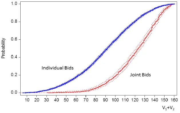
(17) breakdown). Aggregate results and results at the regional scenario level show a high degree of conformity. For this reason, we provide the disaggregated data for the interested reader, but only briefly discuss them in the robustness section. We begin by comparing the base treatment with joint bids (T0) to the treatment without joint bids (T1) corresponding to the first two columns in Tables 2-7. In the robustness section, we discuss three additional treatments (last three columns in Tables 2-7). We start by describing bidding behavior and follow with an analysis of winning bids and their effect on auction revenue and efficiency. 4.1. General Bidding Patterns. When comparing columns one and two in Table 2, a couple of preliminary observations are worth making. When joint bidding is allowed, about one out of five bids are joint. This demonstrates that players make extensive use of joint bids. Recall that joint bidders have to overcome two hurdles: (a) non-trivial search to find a player with ‘strategically attractive’ valuations in order to increase the gains from joint bidding (b) bargaining under asymmetric information in order to share the joint surplus. As a benchmark, note that if all possible joint bid opportunities were exploited, a session of ten auctions would produce 140 joint bids and 50 single bids (lots with three potential bidders necessarily force single bids). Thus, the maximum possible proportion of joint bids in the data is 73.7%. It is difficult to say whether the observation that 19,4% of bids submitted in T0 is high or low relative to that upper bound. What is important, however, is that this figure is large enough to have an economically significant impact on revenue and efficiency. As expected, joint bidders have higher combined valuations than individual bidders. Figure 3 plots the empirical cumulative distribution of lots valuations for individual and joint bidders. The former stochastically dominates the later. Taking averages, joint bidders have valuations that are about 30% higher than individual bidders (120.5 vs. 86.5). Several effects are at play. One effect was illustrated earlier with Figure 2 under the assumption of random matching. That’s not the only effect, however. Joint bids are not drawn from a random sample of valuations. To start, those who enter joint bidding agreements have private lot valuations (prior to agreeing to bid jointly) that are greater than individual bidders (88 versus 76 and the difference is statistically significant). But this is not the only way that the actual matching departs from the random benchmark. Each participant in a joint bid has valuations for the two goods that are more heterogeneous than individual bidders. For example, the absolute difference between the two good values ( v1i  v2i ) for players who make joint bids is 34, while it is only 24 for individual bidders (and the difference is highly significant).. 14.

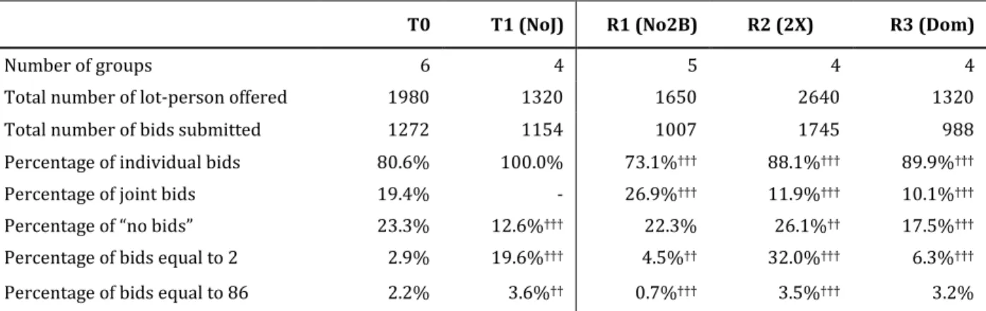
(18) Figure 2: Empirical CDF (with Confidence Intervals) of Individual and Join Bidder Values. Turning to bidding behavior, note that the percentage of lots with no bids is higher in the joint bid treatment (23.3% versus 12.6%) and the percentage of bids equal to two is lower (2.9% against 19.6%). Interestingly, the two effects go in opposite direction. When players cannot make joint bids, they often make bids of two instead of no bid. It could be that collusive bidding significantly increases when joint bids are not allowed. One may question whether the bids of two are indeed a sign of collusion. Under the collusion hypothesis, a bid of two is an umbrella to shield another (higher) collusive bid from the two bidder rule. Thus, if bids of two are collusive, they should happen in conjunction with less aggressive bids on the same lot. This leads to the hypothesis that bids and bid-to-value ratios of bids greater than 2 should be lower when there is a bid of two on a lot. This prediction is unique to the collusion hypothesis. To test this hypothesis, we divide the bids greater than two between those for which another bidder has submitted a bid of two on the same lot, and those for which no bid of two was submitted. When joint bids are allowed (T0), we find that the average bid is 72.5 when there is a bid of two on the same lot and 76.0 when it’s not the case. The difference for bid-to-value ratios is even more pronounced (70.9% versus 79.3%). When joint bids are not allowed (T1) the same pattern emerges. Bids average 64.4 when a bid of two is submitted and 68.9 otherwise; the bid-tovalue ratios are 68.5% and 76.7% respectively. As expected, there is less competition on lots for which a bid of two is made. This offers some evidence in support of the collusion hypothesis. 15.

(19) Third, the proportion of bids equal to the announced starting price of 86 is slightly higher when joint bids are not allowed. Bidders bid 86 to ensure that they are not subject to the two bidder rule. Thus, it would appear that prohibiting joint bidding increases the frequency of collusive behavior, but also leads to a greater number of bids where individuals without a market splitting agreement feel compelled to bid 86 to avoid the risk of being disqualified if no other player submitted a bid. Table 2: Summary of Observations and Bid Types Per Treatment T0. T1 (NoJ). R1 (No2B). 6. 4. 5. 4. 4. Total number of lot-person offered. 1980. 1320. 1650. 2640. 1320. Total number of bids submitted. 1272. 1154. 1007. 1745. 988. 88.1%†††. 89.9%†††. Number of groups. R2 (2X). R3 (Dom). Percentage of individual bids. 80.6%. 100.0%. 73.1%†††. Percentage of joint bids. 19.4%. -. 26.9%†††. 11.9%†††. 10.1%†††. Percentage of “no bids”. 23.3%. 12.6%†††. 22.3%. 26.1%††. 17.5%†††. Percentage of bids equal to 2. 2.9%. 19.6%†††. 4.5%††. 32.0%†††. 6.3%†††. Percentage of bids equal to 86. 2.2%. 3.6%††. 0.7%†††. 3.5%†††. 3.2%. Note: Levels of statistical significance when compared to T0 are †:p< 0.1; ††:p< 0.05; and. †††:. p<0.01.. 4.2 Bids and bid-to-value ratios We now turn our attention to bid levels across T0 and T1. Figure 3 plots all positive bids as a function of the bidder(s)’ underlying total value for the lot. It allows for a bird’s eye view of the dataset, with individual bids showing in clear dots and joint bids in dark dots. Several interesting patterns emerge. To start, most bids are below the 45 degree line. This shows that bids giving negative expected profits (that could be mistakes due to inattention, for example) are rare. More interestingly, bids are roughly monotone and increasing in valuation with a mild concave shape over high valuations. A monotonically increasing equilibrium bidding function is the norm in auction theory and auction experiments as well. Moreover, the graphs reveal the high number of bids equal to two (horizontal line at two) previously noted. Two further points emerge: there are very few data points between the line at two and the main cloud just below the 45 degree line. This further supports the collusion hypothesis. One would have expected more continuity between these two sets of points under the ‘market scooping’ hypothesis. Moreover, some of the players with very high valuations make bids equal to two and this is particularly pronounced in T1. This is surprising because these lots carry a high probability of a win and therefore high expected profits in a normal auction. Again, it is difficult to rationalize this behavior without appealing to a market splitting argument.. 16.

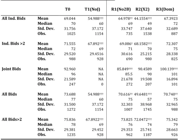
(20) Tables 3 and 4 more precisely describe the difference in bidding behavior between T0 and T1, presenting individual and joint bids together and separately. Averages expressed in experimental dollars are presented in Table 3, while Table 4 is expressed as the bid-to-value ratios. We report statistics on all individual bids as well as those greater than 2 only in order to separate the effects of strategic bids. Table 3 reveals important differences in bidding behavior: (1) Overall bids are much higher when joint bids are allowed (73.7 versus 55.0) and this holds even when we consider only bids above two (75.8 versus 67.9). (2) In the joint bid treatment, joint bids are significantly higher than solo bids (93.0 versus 69.0). (3) Even when we compare individual bids above two, we still find higher bids when joint bid are allowed (71.6 versus 67.9). Allowing joint bids generates an asymmetry where joint bids dominate individual bids and it increases the overall aggressiveness of bids of both joint and individual bidders. Table 4 further establishes this point by looking at bid to value ratios. All bidders bid a larger fraction of their value when joint bids are allowed (79.0% versus 75.6%). Individual bidders also bid a larger fraction of their valuation in the joint bid treatment (they bid 78.7% in T0 versus 75.6 % of their valuation in T1), consistent with standard predictions for weak bidders.. However, joint bids in T0 are also more aggressive than individual bids in T0, a fact not easily reconciled with their dominant bidder position in an auction they know has one fewer potential bidder.. 17.

(21) Figure 3: Individual and Joint Bids by Treatment. No Joint Bid (T1). Bid. Bid. Base Treatment (T0). V1 + V2. V1 + V2. Double Supply – (R2). Bid. Bid. No 2-Bidder Rule (R1). V1 + V2. V1 + V2. Players Without Penalty (R3). V1 + V2. 18.

(22) Table 3: Descriptive Statistics of Bids T0. T1(NoJ). R1(No2B). R2(X2). R3(Dom). All Ind. Bids. Mean Median Std. Dev. Obs.. 69.044 70 31.756 1025. 54.988††† 60 37.172 1154. 64.978†† 44.1554††† 69 49 33.747 37.640 735 1538. 67.3923 72 32.689 887. Ind. Bids >2. Mean Median Std. Dev. Obs.. 71.555 72 29.520 988. 67.892††† 69 29.4516 928. 69.086† 68.1582††† 71 70 30.616 25.215 690 980. 72.307 75 28.338 825. Joint Bids. Mean Median Std. Dev. Obs.. 92.960 96 21.589 247. NA NA NA 0. All Bids. Mean Median Std. Dev. Obs.. 73.688 77 31.500 1272. All Bids>2. Mean Median Std. Dev. Obs.. 75.836 78 29.381 1235. 85.849††† 85.5 21.678 272. 90.4589 90 19.508 207. 100.139††† 101 16.894 101. 54.988††† 60 37.172 1154. 70.616†† 49.6481††† 75 57 32.303 38.968 1007 1745. 70.740†† 75 32.965 988. 67.8922††† 69 29.452 928. 73.825 72.0472††† 76 74 29.353 25.741 962 1187. 75.342 79 28.663 926. Level of statistical confidence when compared to T0: †:p< 0.1; ††:p< 0.05; and. †††. : p<0.01.. Table 4: Descriptive statistics of Bid-to-Value ratios for bids greater than two T0. T1(NoJ). R1(No2B). R2(X2). R3(Dom). Ind. Bids. Mean Median Std. Dev. Obs.. 0.7870 0.8182 0.1448 988. 0.7561††† 0.7924 0.1646 928. 0.7631††† 0.7971 0.1493 690. 0.6901††† 0.7059 0.1306 980. 0.8055††† 0.8333 0.1497 825. Joint Bids. Mean Median Std. Dev. Obs.. 0.8013 0.8130 0.1122 247. NA NA NA 0. 0.7510††† 0.7608 0.0932 272. 0.7176††† 0.7391 0.0992 207. 0.7882 0.7928 0.0879 101. All bids. Mean Median Std. Dev. Obs.. 0.7899 0.8156 0.1389 1235. 0.7561††† 0.7924 0.1646 928. 0.7597††† 0.7813 0.1359 962. 0.6949††† 0.7101 0.1261 1187. 0.8036†† 0.8265 0.1444 926. Level of statistical confidence when compared to T0: †:p< 0.1; ††:p< 0.05; and. 19. †††. : p<0.01..

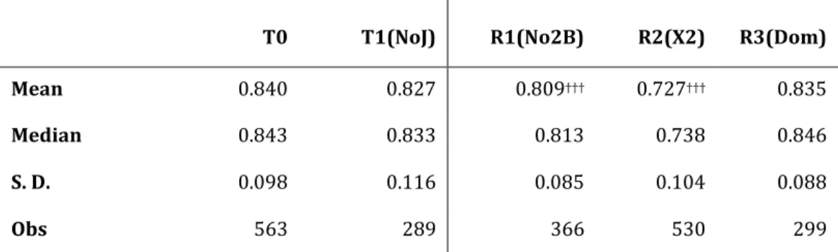
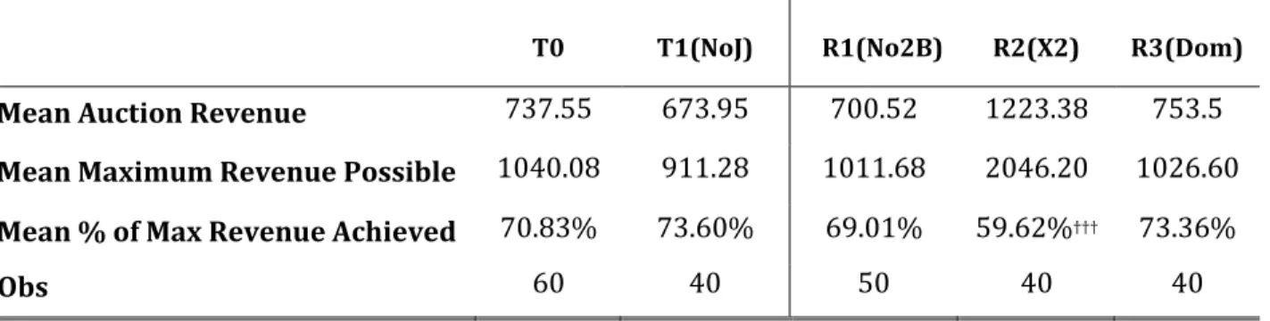
(23) 4.3 Auction Performance: Revenue The bid-to-value ratios identified above provide a representation of the competitive pressure felt by bidders. Ultimately, however, only the winning bids determine the overall performance of the auction in terms of the seller’s revenue. Table 5 reports the bid-to-value ratio of lots won and allocated in the auctions. The data presented are to be interpreted as the descriptive statistics of the proportion of winner’s value that is captured by the seller through the sale price (thus excluding lots not sold). Table 5: Descriptive Statistics; Revenue per lot as a fraction of winner’s value T0. T1(NoJ). R1(No2B). R2(X2). R3(Dom). Mean. 0.840. 0.827. 0.809†††. 0.727†††. 0.835. Median. 0.843. 0.833. 0.813. 0.738. 0.846. S. D.. 0.098. 0.116. 0.085. 0.104. 0.088. Obs. 563. 289. 366. 530. 299. Level of statistical confidence when compared to T0: †:p< 0.1; ††:p< 0.05; and. †††. : p<0.01.. Winners in T1 bid on average the same proportion of value as winners in the base treatment (84% and 82.6% are not statistically different). Recall, however, that the distribution of valuation in T0 stochastically dominates the distribution of valuation in T1. Thus, while the profit margins on the lots are equal, the total revenue in T1 are bound to be lower since no valueenhancing joint bids can be formed. This is confirmed in the first line of Table 6, showing that the absence of joint bids depresses winning bids (the mean auction revenue is 673.9 versus 737.5). The next row in Table 6 shows that the maximum possible mean revenue is 1040.1 for the joint bid treatment but only 911.28 without joint bids. This is computed differently for the no joint bid treatment and all other treatments. For T1 it is computed as the average across all auctions of the sum of the highest individual valuations across all potential bidders. This maximum total revenue, therefore, is simply the revenue the seller would have obtained if the bidder with the highest value won the lot and paid exactly that value. For the other four treatments, the maximum possible revenue is the sum over all lots of the highest possible total value, where the values of the two goods do not have to be from the same bidder (i.e. allowing of the highest values to come from joint bids whenever beneficial). The last line shows the mean over all auctions of the percentage of revenue in an auction divided by the maximum possible revenue (this mean of the ratios is close. 20.

(24) but not exactly the same as the ratio of the means obtained by dividing numbers in line 1by those in line 2). The results confirm that when joint bids are prohibited, a similar proportion of potential revenue is actually achieved, but overall revenue are substantially smaller than when joint bids are allowed. This is the result of the inability of bidders to form welfare enhancing joint bids. Table 6: Average Auction Revenue as a fraction of Maximum Possible Revenue T0. T1(NoJ). Mean Auction Revenue. 737.55. 673.95. Mean Maximum Revenue Possible. 1040.08. Mean % of Max Revenue Achieved. R2(X2). R3(Dom). 700.52. 1223.38. 753.5. 911.28. 1011.68. 2046.20. 1026.60. 70.83%. 73.60%. 69.01%. 59.62%†††. 73.36%. 60. 40. 50. 40. 40. Obs. R1(No2B). Level of statistical confidence when compared to T0: †:p< 0.1; ††:p< 0.05; and. †††. : p<0.01.. 4.4 Auction Performance: Efficiency Of importance to economists and policy makers is the ability of auctions to efficiently allocate the lots being sold. In the case of forestry auctions for bundled goods, one important criterion to judge the different auctions is their ability to allocate each lot and its component parts to the bidder with highest value (allocative efficiency). The benchmark used for computing the level of efficiency realized in our auctions is the optimal allocation of each good for that auction, net of the reserve price of the seller (forest plots are not lost if not sold), and accounting for the penalties imposed by allocating more than four lots per bidder.6 We compare the gains in this benchmark allocation against the gains actually realized empirically by players in each auction. This is equal to the sum of the values realized by buyers for all of the goods sold, minus, once again, the reserve price of sold lots and the penalties assessed on players. To normalize the results across auctions, we take the 6. The optimal allocation for each auction was computed first by allocating each good (i.e. half lot) in the auction to the participant with the highest value for that good. If the sum of the highest two values was lower than the lot’s reserve price, it would be suboptimal to sell it and the lot would remain unsold in the final allocation. Once this initial allocation was computed, each player’s resulting penalties was assessed. Remember that penalties in our design are meant to represent true costs (transactions or otherwise) associated with purchasing stands in excess of capacity. As a result, penalties resulting from the allocation need to be subtracted from the value of stands in the allocation. However, the existence of penalties triggered an algorithm exploring whether any good that marginally triggered a penalty of 10 could be reassigned to the next highest value user. An allocation is superior to the initial allocation if a player can be found who has a value for the good no more than 10 below the value of the initial buyer, and where reallocating the good to this user would eliminate the initial penalty but not trigger one to the new player. Hence, in a two step process, the initial allocation is re-optimized and reallocations made when a penalty can be avoided at a cost of less than 10.. 21.

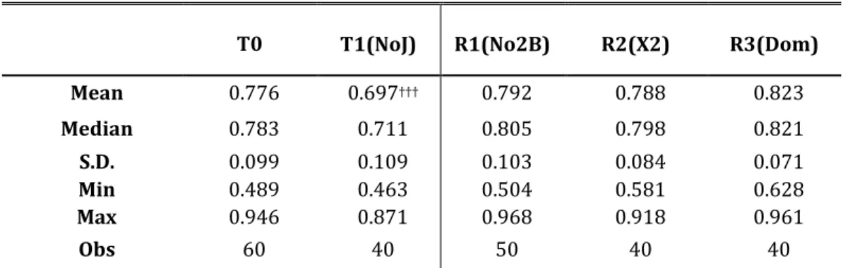
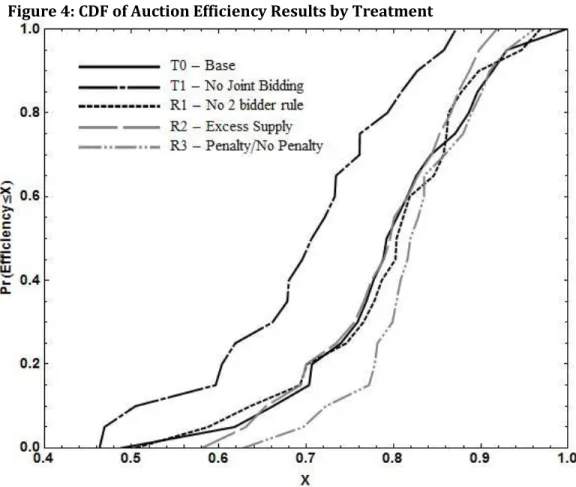
(25) ratio of realized surplus to the surplus in the optimal allocation. The result is an efficiency index between zero and one. Table 7 presents the descriptive statistics and Figure 4 pictures the cumulative distributions of efficiency levels for the different treatments. Inspection of those results reveals a significant drop in efficiency when joint bids are not allowed. Looking at means, for example, reveals an efficiency level of 77.6% with joint bids and 69.7% without joint bids. The baseline level of efficiency of 69.7% is due to the facts that lots are sometimes unallocated, not allocated to the highest bidder, or penalties are imposed. Despite these costs and the complexity or having 8 lots, T1 captures a significant fraction of the potential surplus. The main point, however, is that allowing joint bids increases overall efficiency by more than 10 percentage points, which is an economically significant improvement. Table 7: Efficiency Level per Auction. T0. T1(NoJ). R1(No2B). R2(X2). R3(Dom). Mean. 0.776. 0.697†††. 0.792. 0.788. 0.823. Median. 0.783. 0.711. 0.805. 0.798. 0.821. S.D. Min Max. 0.099 0.489 0.946. 0.109 0.463 0.871. 0.103 0.504 0.968. 0.084 0.581 0.918. 0.071 0.628 0.961. Obs. 60. 40. 50. 40. 40. Level of statistical confidence when compared to T0: †:p< 0.1; ††:p< 0.05; and. 22. †††. : p<0.01..

(26) Figure 4: CDF of Auction Efficiency Results by Treatment. 5. Robustness: No Two Bidder Rule, Excess Supply, and Capacity Constraint As we have seen, joint bidding has a significant and positive impact on bid levels, revenue and efficiency in the experimental setting of our auctions. Are these effects sensitive to the characteristics of the auction environment? Furthermore, it is worth asking whether those results hold across the various regional scenarios. The appendix breaks down the results across the four regional distributions of players and lots. Each distribution has eight lots (sixteen in R2) and six players. When comparing T0 and T1, all of our conclusions hold in each regional scenario in the sense that the direction of the impact of allowing joint bidding remain the same (though in some cases, the smaller sample sizes make the differences not statistically significant). In this section, therefore, we turn to a comparison of the results in three robustness treatments against the baseline treatment (T0). The first robustness looks at the effect of the two-bidder auction rule, while the other two modify the general level of competition between players: R2 doubles the number of lots offered; R3 removes the soft capacity constraint (penalties for buying more than 4 goods) on two players (one in each “region”).. 23.

(27) 5.1 No Two Bidder Rule (R1) Referring back to Table 2, note that removing the two-bidder rule leads to an increase in the propensity to bid jointly (27% versus 19% of joint bids), a decrease in bids at the starting price of 86 and a small increase in the number of bids equal to two. We do not have a solid explanation for the increase in the proportion of bids submitted jointly, although it may be argued that joint bids below 86 for mid-value lots have a relatively small chance of success when there are only three potential bidders and the two-bidder rule is in place. The significant difference in the proportion of bids equal to 86 demonstrates that players understand the strategic value of bidding the starting price of 86 to escape the two bidder rule under T0. More importantly, Tables 4 and 5 show that players bid less aggressively in the absence of the two bidder rule. As a result, auction revenue is lower on average (700.5 versus 737.6 and the difference is not significant but this is partly explained by the fact that the number observations drops dramatically when we aggregate data at the auction level). There is no significant change in efficiency, however. We conclude that the two bidder rule increases bid aggressiveness and auction revenue but does not affect efficiency. 5.1. Excess Supply (R2). R2 differs from T0 in two dimensions: the length of the communication period and the number of lots offered. Thus, we compare R2 both with T0 and with two additional sessions of T0 ran using communication periods that are of the same length as in R2 (not shown here). The main conclusions do not change when we hold constant the length of the communication period. Increasing the supply of lots offered significantly decreases the proportion of bids that are joint and increases significantly the number of bids at two (32% of bids are equal to two against 2.2% in T0).7 Again, we check the collusion hypothesis by comparing the average bid level and bid-to-value ratio for bids that are made on a lot where a bid of two is also entered and for lots where no such bid is made. Although bid levels are similar across the two groups, we find a significant difference in bid-to-value ratios (65.1% versus 71.2%). Again, we find less aggressive bidding on lots for which a bid of two is entered. Taken together, these results hint at a significant lack of competitive bidding and an increase in collusive behavior when there is excess supply. Consistent with this interpretation, Table 5 shows that bidders bid a smaller fraction of their valuation and Table 6 shows a significant decrease in revenue as a fraction of maximum possible revenue. Efficiency levels in this treatment are only marginally lower that in T0 and the difference is not statistically significant. Thus, while collusion significantly affected revenue, it does not affect the auctions’. This difference could be due to the longer communication period, but in the two additional sessions of T0 conducted with equally long communication periods, the proportion of bids at 2 was observed to be 2.7% and thus cannot explain the vast increase observed in R2. 7. 24.

(28) efficiencies. It suggests that despite their anti-competitive nature, the bidding rings formed in this treatment are effective at allocating goods to the player with the highest value. To sum up, a decrease in the overall level of competition caused by excess supply induces more collusion, lower auction revenues, but does not change efficiency. This clearly indicates the importance of maintaining a tight control over the supply of lots in an auction, since excess supply makes it easier for players to divide the market and avoid competition for lots. In the context of field auctions, this makes it more difficult to properly manage public forests. On the one hand, supply must be sufficiently tight to create scarcity and competition on the auction market, but this runs the risk of choking the industry if the supply of timber is accidently set too low to allow proper functioning of the industry. In general, mills should be allowed to maintain private forest reserves or baseline access to public forests, making the auction the source of their marginal supply needs only. Auctions can be used as the instrument of marginal sales from which stumpage fees can be set for the baseline supply as well. 5.2. Unconstrained Players (R3). Unconstrained players do not face a penalty for purchasing more than two lots like other players do. De facto, these players can realize the full face value of a lot while the other players must adjust their bidding to account for expected losses once the two lot capacity has been reached. Much like the formation of joint bids creates strong and weak players, removing the penalties for two players in a group can be thought also as creating strong and weak players. The treatment with unconstrained players has fewer joint bids and slightly more bids of two relative to T0. Efficiency is higher although the difference is not significant. This is likely attributable to the lower overall penalties resulting from removing the capacity constraint on two players. 6. Summary and Conclusions We study the impact of allowing joint bidding in simultaneous multi-units first price sealed bid auctions for bundled goods on bidding behavior, revenue and efficiency. Joint bidding resulted in higher valuations for the lots, and higher bids for them, but overall, winning bids came in as similar proportions of the underlying values. The efficiency gains from joint bidding clearly outweighed the reduction in competition that takes place when two bidders become one or when players collude. When no joint bids are allowed, participants showed a significant increase in the number of collusive bids, and both total revenue and efficiency fell significantly. The fact that students in short experiments managed to collude should give pause to policy makers and point to the need to carefully monitor anomalous bidding patterns in field auctions. Overall, however, the results suggest that permitting joint bidding can result in substantial efficiency gains and increase revenue for the seller. 25.

(29) The research has immediate applications to forest stands that arbor a mixture of species. The auction treatments capture important environmental conditions and auction rules in the complex but policy relevant context of timber auctions implemented in Quebec. Moreover, we explore the robustness of the results to characteristics of the auction environment that are relevant in the timber auctions context. Excess supply produces the most collusion: while efficiency remained high, winning bids and auction revenues were substantially lower when supply was doubled. The removal of capacity constraints and the removal of the two bidder rule have less impact on the results. Overall, the results support the adoption of the set of rules considered by the government of Quebec in its timber auctions. Although there is little evidence that rules requiring a minimum number of bids are effective at discouraging collusion in the laboratory, the results suggest that these rules can help detecting collusive bidding.. 26.

(30) References Athey, S., and J. Levin. 2001. “Competition and Information in US Forest Service Timber Auctions,” Journal of Political Economy 109(2): 375–417 Athey, S., Levin, J., & Seira, E. 2011. Comparing open and Sealed Bid Auctions: Evidence from Timber Auctions. The Quarterly Journal of Economics, 126(1), 207-257. Baldwin, L.H., R.C. Marshall, and J.-F. Richard, 1997. “Bidder Collusion at Forest Service Timber Sales”, Journal of Political Economy 105(4): 657-699. Brannman, L.E., 1996. “Potential Competition and Possible Collusion in Forest Service Timber Auction”, Economic Inquiry 34: 730-745. Burtraw, D., Goeree, J., Holt, C. A., Myers, E., Palmer, K., & Shobe, W. (2009). Collusion in auctions for emission permits: An experimental analysis. Journal of Policy Analysis and Management, 28(4), 672-691. Canada Competition Act. R.S.C., 1985, c. C-34. http://www.laws.justice.gc.ca/eng/acts/C34/index.html Cassiman, B. and R. Veugelers. (2002). R&D cooperation and spillovers: some empirical evidence from Belgium. American Economic Review, 92 (4) (2002), pp. 1169–1184. Chernomaz, K. 2012. On the effects of joint bidding in independent private value auctions: An experimental study. Games and Economic Behavior 76(2):690–710. d'Aspremont, C. and A. Jacquemin. (1988). Cooperative and noncooperative R&D in duopoly with spillovers. American Economic Review, 78 (5) (1988), pp. 1133–1137. Duso, T., Roeller, L., & Seldeslachts, J. (2010). Collusion through Joint R&D: An Empirical Assessment. Tinbergen Institute Discussion Paper 10-112/1. Farrell, J., and Shapiro, C. (1990). Horizontal Mergers: An Equilibrium Analysis. The American Economic Review, 80(1), 107-126. Fischbacher, U. (2007). z-Tree: Zurich toolbox for ready-made economic experiments. Experimental Economics, 10(2), 171-178. Gugler, K., and Siebert, R. (2007). Market Power Efficiency Effects of Mergers and Research Joint Ventures: Evidence from the Semiconductor Industry. The Review of Economics and Statistics, 89(4), 645–659. Gupta, S. (2001). The effect of bid rigging on prices: a study of the highway construction industry. Review of Industrial Organization, 19, 453–467. Gupta, S. (2002). Competition and collusion in a government procurement auction market, Atlantic Economic Journal, 30, 13–25.Haile, P. 2001. “Auctions with Resale Markets: An Application to US Forest Service Timber Sales,” American Economic Review 91: 399–427.. 27.

(31) Hendricks, K., and Porter, R. H. (1989). Collusion in Auctions. Annals of Economics and Statistics, 15/16, 217-230. Isaac, R. M., & Walker, J. M. 1985. Information and conspiracy in sealed bid auctions. Journal of Economic Behavior & Organization, 6(2), 139-159. Kamien, M. and E. Muller, I. Zang. (1992). Research joint ventures and R&D cartels. American Economic Review, 82 (5) (1992), pp. 1293–1306. Kwasnica, A. M. (2000). The choice of cooperative strategies in sealed bid auctions. Journal of Economic Behavior & Organization, 42(3), 323-346. Lebrun, B., 1999. First price auctions in the asymmetric n bidder case. International Economic Review 40, 125–142. Maskin, E., Riley, J., 2000. Asymmetric auctions. Review of Economic Studies 67, 413–438. Moody, C. E. Jr. and Kruvant, W. J. (1988). Joint Bidding, Entry, and the Price of OCS Leases. The RAND Journal of Economics, 19(2), 276-284. Li, T., & Perrigne, I. 2003. Timber sale auctions with random reserve prices. Review of Economics and Statistics, 85(1), 189-200. Mead, W. J. 1967. “Natural Resource Disposition Policy: Oral Auctions vs. Sealed Bids,” Natural Resource Journal 7:194–224. Paarsch, H. 1991. “Empirical Models of Auctions and an Application to British Columbia Timber Sales,” University of British Columbia mimeo. Porter, R. and Zona D. (1993). Detection of bid rigging in procurement auctions. Journal of Political Economy, 101, 518–538. Saphores, J. D., Vincent, J. R., Marochko, V., Abrudan, I., Bouriaud, L., & Zinnes, C. 2007. Detecting Collusion In Timber Auctions: An Application To Romania. World Bank Research Working papers, 1(1), 1-58. Suetens, Sigrid. (2005). Cooperative and non-cooperative R&D in experimental duopoly markets. International Journal of Industrial Organization, 23, 63– 82. Suetens, Sigrid. (2008). Does R&D cooperation facilitate price collusion? An experiment. Journal of Economic Behavior & Organization, 66, 822–836.. 28.

(32) Appendix Table A1 Bids Submitted Jointly. Regional Scenario. T0 (Control) T1(No2B) 0.188 0.202 57 50 304 247. T2(2X) 0.102††† 43 420. T3(NoJ) NA NA 264. T4(Dom) 0.089††† 21 235. 0.282†† 57 202. 0.135† 45 333. NA NA 229. 0.117†† 23 197. 0.216 88 408. 0.302††† 96 318. 0.127††† 72 567. NA NA 374. 0.105††† 33 314. % of bids=joint # of bids=joint Total # of Bids. 0.172 52 302. 0.288††† 69 240. 0.111†† 47 425. NA NA 287. 0.099†† 24 242. % of bids=joint # of bids=joint Total # of Bids. 0.194 247 1272. 0.270††† 272 1007. 0.119††† 207 1745. NA NA 1154. 0.102††† 101 988. 2-0-6. % of bids=joint # of bids=joint Total # of Bids. 2-3-3. % of bids=joint # of bids=joint Total # of Bids. 0.194 50 258. 2-4-2. % of bids=joint # of bids=joint Total # of Bids. 2-6-0. All. Level of statistical confidence when compared to T0: †:p< 0.1; ††:p< 0.05; and. †††:. p<0.01.. Table A2 Data on Bids=2. Regional Scenario. 2-0-6. % of Bids=2 # of Bids=2 Total # of Bids. T0 (Control) 6.58 20 304. T1(No2B) 4.45 11 247. T2(2X) 35.48††† 149 420. T3(NoJ) 26.14††† 69 264. T4(Dom) 16.60††† 39 235. 2-3-3. % of Bids=2 # of Bids=2 Total # of Bids. 3.88 10 258. 3.47 7 202. 28.83††† 96 333. 18.34††† 42 229. 2.54 5 197. 2-4-2. % of Bids=2 # of Bids=2 Total # of Bids. 0.98 4 408. 3.77†† 12 318. 31.22††† 177 567. 16.31††† 61 374. 4.78††† 15 314. 2-6-0. % of Bids=2 # of Bids=2 Total # of Bids. 0.99 3 302. 6.25††† 15 240. 32.00††† 136 425. 18.82††† 54 287. 1.24 3 242. All. % of Bids=2 # of Bids=2 Total # of Bids. 2.91 37 1272. 4.47†† 45 1007. 31.98††† 558 1745. 19.58††† 226 1154. 6.28††† 62 988. Level of statistical confidence when compared to T0: †:p< 0.1; ††:p< 0.05; and. 29. †††:. p<0.01..

(33) Table A3 Data on Bids=86. Regional Scenario. 2-0-6. % of Bids=86 # of Bids=86 Total # of Bids. T0 (Control) 3.29 10 304. T1(No2B) 0.81†† 2 247. T2(2X) 5.24 22 420. T3(NoJ) 3.41 9 264. T4(Dom) 4.68 11 235. 2-3-3. % of Bids=86 # of Bids=86 Total # of Bids. 2.71 7 258. 0.50† 1 202. 3.00 10 333. 4.80 11 229. 4.06 8 197. 2-4-2. % of Bids=86 # of Bids=86 Total # of Bids. 1.96 8 408. 0.63 2 318. 2.65 15 567. 4.01† 15 374. 2.55 8 314. 2-6-0. % of Bids=86 # of Bids=86 Total # of Bids. 0.99 3 302. 0.83 2 240. 3.29†† 14 425. 2.44 7 287. 2.067 5 242. All. % of Bids=86 # of Bids=86 Total # of Bids. 2.20 28 1272. 0.70††† 7 1007. 3.50†† 61 1745. 3.64†† 42 1154. 3.24 32 988. Level of statistical confidence when compared to T0: †:p< 0.1; ††:p< 0.05; and. †††:. p<0.01.. Table A4 Descriptive Statistics All Bids >2 T0 (Control). T1(No2B). T2(2X). T3(NoJ). T4(Dom). 2-0-6. Mean S.D. Obs.. 75.306 28.158 284. 71.805 30.470 236. 69.173 22.933 271. 66.610 28.797 195. 74.066 28.863 196. 2-3-3. Mean S.D. Obs.. 75.875 27.957 248. 69.897 28.821 195. 74.0338 25.956 237. 69.529 28.043 187. 72.432 28.736 192. 2-4-2. Mean S.D. Obs.. 76.606 30.819 404. 75.431 29.252 306. 72.7974 26.120 390. 66.981 30.197 313. 78.027 26.476 299. 2-6-0. Mean S.D. Obs.. 75.264 29.800 299. 77.164 28.380 225. 72.1004 27.390 289. 68.876 30.167 233. 75.368 30.871 239. All. Mean S.D. Obs.. 75.836 29.381 1235. 73.825 29.353 962. 72.047 25.741 1187. 67.892 29.452 928. 75.342 28.663 926. Regional Scenario. Level of statistical confidence when compared to T0: †:p< 0.1; ††:p< 0.05; and. 30. †††:. p<0.01..

(34) Table A5 Descriptive Statistics for Bid/Value WINNING BIDS ONLY T0 (Control) T1(No2B). Regional Scenario. T2(2X). T3(NoJ). T4(Dom). 2-0-6. Mean S.D. Obs.. 0.827 0.121 123. 0.818 0.101 105. 0.714††† 0.1028 143. 0.827 0.099 76. 0.816 0.104 87. 2-3-3. Mean S.D. Obs.. 0.842 0.064 84. 0.814†† 0.083 70. 0.743††† 0.105 103. 0.824 0.121 62. 0.847 0.080 59. 2-4-2. Mean S.D. Obs.. 0.849 0.108 130. 0.803† 0.078 113. 0.721††† 0.105 171. 0.842 0.131 91. 0.841 0.084 93. 2-6-0. Mean S.D. Obs.. 0.846 0.066 86. 0.801††† 0.0745 78. 0.740††† 0.101 113. 0.810††† 0.108 60. 0.844 0.071 60. All. Mean S.D. Obs.. 0.840 0.098 423. 0.809††† 0.085 366. 0.727††† 0.104 530. 0.827 0.116 289. 0.835 0.088 299. Level of statistical confidence when compared to T0: †:p< 0.1; ††:p< 0.05; and. 31. †††:. p<0.01..

(35)