HAL Id: halshs-01074934
https://halshs.archives-ouvertes.fr/halshs-01074934v2
Preprint submitted on 26 Mar 2015HAL is a multi-disciplinary open access archive for the deposit and dissemination of sci-entific research documents, whether they are pub-lished or not. The documents may come from teaching and research institutions in France or abroad, or from public or private research centers.
L’archive ouverte pluridisciplinaire HAL, est destinée au dépôt et à la diffusion de documents scientifiques de niveau recherche, publiés ou non, émanant des établissements d’enseignement et de recherche français ou étrangers, des laboratoires publics ou privés.
Gender Preferences in Africa: A Comparative Analysis
of Fertility Choices
Pauline Rossi, Léa Rouanet
To cite this version:
Pauline Rossi, Léa Rouanet. Gender Preferences in Africa: A Comparative Analysis of Fertility Choices. 2015. �halshs-01074934v2�
WORKING PAPER N° 2014 – 33
Gender Preferences in Africa:
A Comparative Analysis of Fertility Choices
Pauline Rossi
Léa Rouanet
JEL Codes: I1, J13, J16, O55
Keywords: Gender preferences, Fertility, Africa
P
ARIS-
JOURDANS
CIENCESE
CONOMIQUES48, BD JOURDAN – E.N.S. – 75014 PARIS
TÉL. : 33(0) 1 43 13 63 00 – FAX : 33 (0) 1 43 13 63 10
Gender Preferences in Africa:
A Comparative Analysis of Fertility Choices
Pauline Rossi and L´ea Rouanet
∗February 2015
Abstract
This paper proposes a new method to infer gender preferences from birth spacing. We apply it to Africa, where the least is known about gender preferences. We show that son preference is strong and increasing in North Africa. By contrast, most Sub-Saharan African countries display a preference for variety or no preference at all. Further analysis concludes that traditional family systems predict well the nature of gender preferences, while religion does not. Last, the magnitude of preferences is stronger for wealthier and more educated women.
Keywords: Gender preferences, Fertility, Africa. JEL Codes: I1, J13, J16, O55.
∗Both authors are at Paris School of Economics and CREST. Address: Paris School of Economics, 48
Boulevard Jourdan, 75014 Paris, France. Emails: pauline.rossi@ensae.fr; lea.rouanet@ensae.fr. Corresponding author: Pauline Rossi; tel: +33 1 43 13 63 64; fax: +33 1 43 13 63 55. For their careful reading of our paper and their numerous suggestions, we are grateful to Denis Cogneau, Xavier d’Haultfoeuille and Sylvie Lambert. We also benefited from discussions with V´eronique Hertrich and seminar participants at Paris School of Economics and CREST.
In the early 90s, Sen (1990) coined the term « missing women » to draw attention on the excess mortality of women in Asia: he estimated that approximately an extra hundred million women would be there if men and women received similar care in health, medicine, and nutrition. Since then, a large literature focusing mainly on South Asia and East Asia has described the discrimination against girls, mentioning for instance sex-selective abortions (Sen, 2001), differential child mortality (Rose, 1999), or differential health status (Pande,
2003). By contrast, Sub-Saharan Africa appears to do remarkably well. Sex ratios at birth are close to one, and survival rates as well as health outcomes are generally better for girls than for boys (Wamani, Astrom, Peterson, Tumwine, & Tylleskar, 2007; Anderson & Ray,
2010). All this may explain why gender preferences for children in Sub-Saharan Africa are rarely studied.
This paper focuses on fertility behavior as an alternative mechanism generating gender inequality, even when aggregate sex ratios are balanced. In their seminal paper, Ben-Porath and Welch (1976) infer the existence of gender preferences from the correlation between the probability to stop having children and the gender composition of existing ones. The idea has given rise to formal models of differential stopping behavior in favor of sons, predicting that an average girl has more siblings than an average boy1 (Jensen,2005). There might be
important implications for gender inequality because girls would then face more competition for household resources.2
On the other hand, the analysis of differential spacing behavior is of special importance in the African context. Indeed, when couples have many children, gender preferences are more likely to lead to differences in birth intervals rather than in sibship size. Jensen(2005)
1. As a simple example, consider a population in which parents have only one child if the first-born is a boy, and have two children if she is a girl. 50% of couples would have one son, 25% one girl and one son, and 25% two girls. Sex ratio is perfectly balanced at the aggregate level, but at the household level, girls have always one sibling whereas boys have, on average, one third sibling.
2. Differential stopping behavior has been tested and validated by an extensive literature focusing again on Asia: e.g. Clark (2000), Jensen (2005), and D. Basu and Jong (2010) in India, Abrevaya (2009) in the Chinese and Asian Indian populations living in the US, andHatlebakk(2012) in Nepal.
and D. Basu and Jong (2010) advocate looking at birth intervals to find evidence of gender preferences in a high-fertility context. Under son preference, differential spacing behavior implies that an average boy is breastfed longer than an average girl,3 which may translate
into inequality between boys and girls (Jayachandran & Kuziemko, 2011). Another reason to consider birth intervals is to account for health risks related to spacing, and not only to the number of births: according to the medical literature on developing countries, short birth intervals are associated with adverse outcomes for mothers (Conde-Agudelo & Belizan,2000) and children (Conde-Agudelo, Rosas-Bermudez, & Kafury-Goeta, 2006). The authors show that intervals lower than 24 months multiply the risk of infant death by 2.5, and intervals lower than 15 months multiply the risk of maternal death by two. If gender preferences turn out to induce short birth spacing, they could be a significant cause of maternal and infant mortality in Africa.
In this paper, we propose a new method to infer gender preferences from differential birth spacing. We use a duration model of birth intervals to test if the gender composition of previous children influences the duration before the next birth. The main advantage of duration models is to deal properly with right-censored observations, i.e. families that are not yet complete by the time of the survey (Leung,1988,1991). We infer the existence of son (resp. daughter) preference when birth spacing is shorter for couples with fewer sons (resp. fewer daughters) ; and we deduce that preference for variety prevails when couples having a balanced mix of sons and daughters wait longer than couples having same-sex children. The conceptual framework underlying this strategy is a unitary model of the couple4 choosing
3. Again, as a simple example, consider a population in which parents always have two children ; if the first-born is a girl, they try to have another child immediately, while they wait some time if the first-born is a boy. First-born girls, who represent half of the female population, are weaned prematurely while the entire male population is properly breastfed.
4. This is probably a strong assumption given the complexity of marital lives in Africa. In particular, we do not take into account that children might have different fathers, and that those fathers might also have children with other women. We will partly address this issue by comparing polygamous and monogamous women.
optimal spacing and stopping rules. People might have a taste for balance in the gender composition of children, or a girl/boy bias ; then, costs and benefits may differ for sons and daughters. What is labeled as « gender preferences » is the outcome of a decision problem based on tastes and prices. One caveat of this strategy is that preferences are revealed if and only if couples have the means to control birth spacing and/or stopping.5 Using duration
models of birth intervals, son preference has been extensively tested and validated in Asia,6 but not in Africa. To our knowledge, there is no empirical study based on fertility behavior that documents systematically the variation in gender preferences in Africa. We contribute to fill in this gap using Demographic and Health Surveys in 37 African countries.
We find that, in North Africa (Morocco, Tunisia and Egypt), son preference is strong and has increased over time. By contrast, in most Sub-Saharan African countries, behavior is consistent with either preference for variety or no preference. South Africa, in particular, is characterized by a strong taste for balance. There is weak evidence of son preference in Mali, Senegal and in the Great Lakes region, but the impact on fertility patterns is not substantial. We further investigate the role of socioeconomic factors in shaping gender preferences. Wealthier and more educated women display the same type of preferences as the others, but the magnitude of their preferences is much larger. Then, in Sub-Saharan Africa, there is no correlation with religion: Muslims exhibit the same preferences as other religious groups. On the other hand, traditional kinship structure predicts well the nature of preferences: son preference prevails in patrilineal ethnic groups only. Last, gender preferences seem to translate into differential birth spacing mainly through contraception. In North Africa, modern contraceptive users display a significantly stronger son preference than non-users. In Sub-Saharan Africa, contraceptive users exhibit preferences for variety whereas we
5. In Section 4.3, we discuss the different mechanisms through which gender preferences may translate into differential spacing.
6. E.g. in China (Tu, 1991), in Bangladesh (Rahman & DaVanzo., 1993), in the Chinese population of Malaysia (Pong,1994), in Vietnam (Haughton & Haughton,1995), in India (Arnold, Choe, & Roy.,1998), in South Korea (Larsen, Chung, & Gupta,1998), and in Taiwan (Tsay & Chu,2005).
find no evidence of gender preferences among non-users ; for them, we cannot tell whether they have no preferences or are not able to translate them into fertility choices.
The outline of the paper is as follows. Section 1 provides background on theoretical motives for gender preferences and a review of empirical evidence in Africa. Section 2 presents the data and some descriptive statistics. Section 3 discusses the empirical strategy and the identification assumptions. The main results are reported in Section 4, and some robustness tests are described in Section 5. Section 6 concludes.
1
Gender preferences in Africa
1.1
Theoretical motives for gender preferences
The most important motive put forward by the literature on gender preferences is the traditional structure of family systems. In patrilineal7 and patrilocal8 family systems, men are the fixed points in the social order, so that investment in daughters is considered as investment in another family’s daughters-in-law. In Asia, such a system has produced eco-nomic incentives to have sons. For instance, the money spent for a son’s marriage remains in the family while the dowry paid for a daughter’s marriage is a net expense. In the same vein, female labor force participation is only valued once the daughter is adult, hence bene-fiting the family-in-law.9 Last, sons act as old age insurance for their parents, because they are the ones who remain in the family’s house. They also act as widowhood insurance for their mother, because widows’ claims on the late husband’s resources enjoy a higher social legitimacy if they have sons (Agarwal,1994;Das Gupta et al.,2003). Mothers, in particular, really need a son because their status improves substantially when their sons get married:
7. Main assets are passed on through the male line whereas daughters are given movable goods. 8. Upon marriage, wives move to their husbands’ abode.
9. In a context of child labor, son preference decreases when wages increase in the sectors of activity dedicated to girls (e.g.Koolwal(2007) in Nepal).
they can exert their power over daughters-in-law. Ultimately, women play a dramatic role in the perpetuation and reinforcement of patriarchy. Demographers working on Africa have come to similar conclusions (Lesthaeghe, 1989): among the key factors shaping the repro-ductive regime in this region, they mention traditional inheritance patterns. In matrilineal societies, having daughters is necessary to perpetuate the lineage, whereas families need sons in patrilineal societies. But Africa is different from Asia along at least two dimensions. First, the system of brideprice prevails in almost all ethnic groups: the groom has to pay for the bride, contrary to what happens in a system of dowry. Second, the kinship structure is more flexible: adoptions and exceptions to allow daughters to inherit land in the absence of a son are not unusual in African patrilineal societies. Eventually, the imperative to have a biological son is weaker in Africa than in Asia.
Another motive specific to Africa is the depth of Islamic penetration. In North Africa, the influence of the Islamic law is strong. These societies are characterized by property concen-tration, endogamous marriages and women seclusion, which implies that women’s security and status critically depend on their ability to have sons. In Sub-Saharan Africa, traditions and customs have generally advocated common land ownership, exogamous marriages, wo-men labor participation and wowo-men’s societies, which renders wowo-men less dependent on their sons.(Lesthaeghe, 1989)
The last part of the literature focuses on the impact of modernization factors on gender preferences ; female education and labor participation, access to modern contraceptives, urba-nization, economic growth and mass media are the most studied factors. The modernization hypothesis states that socio-economic development would equalize the value of daughters and sons to their parents, leading to preferences for variety. However, modernization also brings about birth control - promoting smaller family size and facilitating sex-selective reproductive behavior - which could intensify, at least in the short run, traditional gender preferences. So far, the debate is still open, since empirical studies have found mixed results, depending on
the context, the indicator, and the empirical specification they look at.10
1.2
Empirical evidence so far
In her review of the empirical evidence on gender preferences,Fuse(2008) concludes that, although North Africa has not been subject to much research compared to East or South Asia, there is evidence of strong gender bias against girls. She further writes that « of all sub-regions in the world, it appears that the least is known about Sub-Saharan Africa ».
Cross-country analyses generally find evidence of son preference in North Africa, but not in the rest of the continent (see Arnold(1992) on declared preferences and fertility behavior and Chakravarty (2012) on breastfeeding duration). Sub-Saharan Africa is characterized by a female advantage in infant mortality (Anderson & Ray, 2010), as well as in nutritional status and health outcomes (Wamani et al.,2007). It does not display any systematic gender differences in breastfeeding and health seeking behavior (Garenne,2003). Regarding declared preferences,11 Fuse(2008) reports that most women in this region have no ideal gender
com-position, or would prefer to have the same number of sons and daughters. As for household resources, Deaton (1987) found no evidence of differential allocation between boys and girls in Ivory Coast.
Still, some studies show that son preference may appear in Sub-Saharan Africa in case of income shocks. For instance,Flato and Kotsadam(2014) find that infant mortality increases more for girls than for boys during a drought ; they further explain that such a difference is due to discrimination, since the effect is larger in communities more likely to discriminate
10. For instance, modernization factors are associated with smaller son preference in studies on India (Bhat & Zavier,2003), Nepal (Barbar & Axinn,2004), China (Arnold & Liu,1986;Poston,2002), or Egypt (Vignoli,
2006). But other studies on India (Das Gupta, 1987; A. Basu, 1999; Rajan, Sudha, & Mohanachandran,
2000; Jayachandran, 2014), South Korea (Edlund & Lee, 2013), Egypt (Yount, Langsten, & Hill, 2000) or Sub-Saharan Africa (Klasen,1996) have questioned this result.
11. Parents are supposed to have an ideal gender composition of children. Son (resp. daughter) preference is then defined as the ideal number of sons being strictly greater (resp. lower) than the ideal number of daughters.
against daughters (strong declared son preference, preference for a small family size and low female employment). In the same vein, Friedman and Schady(2012) find that girls are more exposed than boys to mortality risk in case of aggregate economic shock.
Last, a specific study on Nigeria shows that women with first-born daughters are significantly more likely to end up in a polygynous union, to be divorced, and to be the head of the household ; they also have significantly more children (Milazzo,2014).
Only a few papers estimate duration models of birth intervals in an African context.12
Gangadharan and Maitra (2003) find evidence of son preference in South Africa, but only among the Indian community. Anthropologists working on the Gabbra, a patrilineal and patrilocal society in Kenya, find that women with no son have shorter birth intervals than women with at least one son (Mace & Sear, 1997). Last, Lambert and Rossi (2014) show that, in Senegal, women most at risk in case of widowhood substantially shorten birth spacing until they get a son. They relate son preference to women’s needs for widowhood insurance. Our paper contributes to the literature using duration models of birth intervals to test systematically for son preference in Africa. So far, evidence is quite limited in this region.
2
Data
2.1
Data
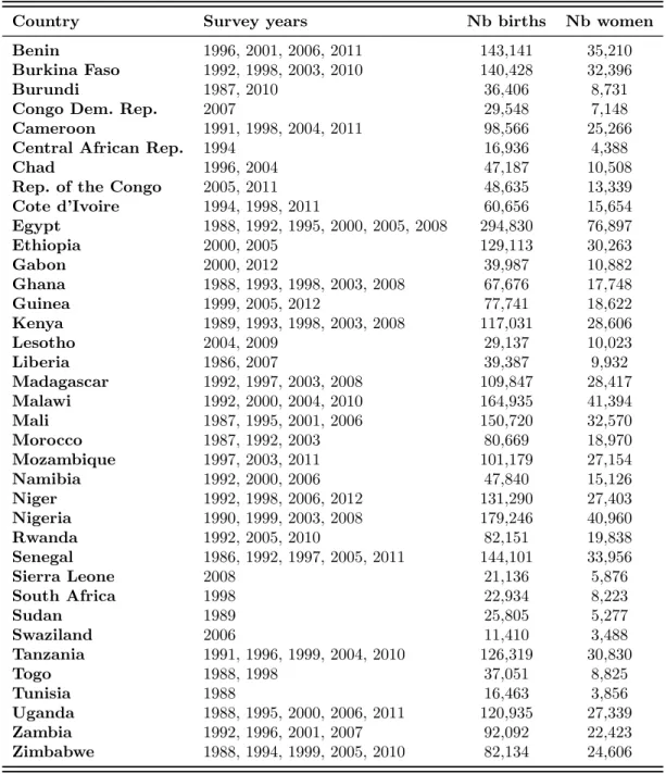
We use DHSsurveys (Demographic and Health Surveys) that were collected from 1986 to
2012 in 37 African countries (surveys listed in Table A.1 in Appendix A). DHSdata contain
stratified samples of mothers aged 15 to 49 who are asked about their reproductive history. DHS data are provided with individual survey weights to ensure that the survey sample is
representative of all mothers at the country level. Nonetheless, sample size of surveys is not
12. Some papers use duration models of birth intervals in Africa, but they are interested in the impact of socio-economic factors (e.g. mother’s characteristics such as birth cohort, age at first marriage and at first birth, residence, education inGhilagaber and Gyimah(2004)), not in son preference.
proportional to population size. To obtain a representative sample of the 37 African countries studied, we reweighed the whole sample.13
The main advantage of these data is that we observe all births, for children either alive or dead at the time of the survey, and we know the year and month of birth of all children, which enables us to measure birth intervals in months. Also, surveys are similar across countries, with a large number of observations (cf. Table A.1 in Appendix A), which allows a comparative analysis.
Nonetheless, the comparative analysis over space and time based on DHS data has two
limits. On the one hand, surveys are not available in all African countries ; notably Algeria, Libya, Mauritania, Eritrea, Somalia, Angola and Botswana are missing. Still, our sample represents 92% of the whole African population in 2009. On the other hand, the surveys took place during a relatively long period of time, so that by pooling the surveys together, we are considering different periods in different countries. In Sub-Saharan Africa, the period of interest is quite homogeneous: in all countries, the majority of mothers are born in the 60s-70s. This is true also in Egypt, but not in other North countries: in Tunisia, Morocco and Sudan, most women are born before 1960.14 We have to keep these caveats in mind
when interpreting cross-country comparisons and time evolutions.
We exploit a second source of data to get information on family systems. We use Mur-dock’s data on African ethnic groups (Murdock, 1959) coded by Gray (1998)15 to define
which women belong to a matrilineal ethnic group. We opted for a conservative definition of matrilinearity, including only those ethnic groups listed by Gray that we found in the DHS
13. Using World Bank population statistics, we compute a sampling rate equal to the number of mothers in the survey implemented in country j and year i, divided by the total population of country j in year i. We also correct for the different number of surveys by country.
14. On the other hand, the fact that we do not observe recent cohorts in Morocco and Tunisia makes our sample more homogeneous: all countries are at a very early stage of the fertility transition.
15. Gray (1998) provides a database that lists the characteristics of African ethnic groups reported by Murdock. Of particular interest for us is the variable Descent : M ajorT ype that indicates whether an ethnic group is patrilineal or matrilineal. Table A.2 in Appendix A gives details of our classification and explains how we matched Gray’s and DHSdata.
data. Patrilinearity is identified by default, and probably includes some matrilineal groups.16
Such a measurement error in our classification of ethnic groups is likely to flatten the dif-ferences between matrilineal and patrilineal groups. So when comparing the two categories, we estimate a lower bound of the difference.
2.2
Descriptive statistics
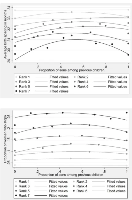
Figure 1 here
Before estimating the duration model, we provide some descriptive statistics of the non-censored durations. The upper graph in Figure 1 represents the average birth spacing by gender composition of the previous children. More precisely, we plot the average duration between births n and (n + 1) as a function of the proportion of boys among the previous n children, for n = 1 to 7. At each rank, birth spacing clearly displays an inverted U-shape:17
it is lower for couples with no son or no daughter, and higher when the sex ratio is balanced. The maximum is reached by couples having slightly more boys than girls.
We find the same pattern when we look at the stopping behavior (cf. lower graph in Figure 1). We plot the proportion of women over 40 years old who stopped having children after the nth birth as a function of the proportion of sons among the previous n children. Here again, women are more likely to stop having children when they already have a balanced mix of boys and girls.
In Appendix A, Table A.3 reports some statistics on fertility stopping and spacing be-haviors, by country. In our sample, women have on average 6.2 children, the average birth
16. We know fromGray(1998) that matrilineal ethnic groups exist in some countries, but the ethnic group variable was missing in DHSdata (e.g. Nigeria, Sudan, Tanzania, Zimbabwe) or DHSdata types were too broad (e.g. DRC) so that we could not identify them.
17. When we regress the non-censored durations on the proportion of boys and the proportion squared, coefficients are significant and of expected sign, whatever rank we consider. We further plot the lines corres-ponding to the quadratic regressions on the graph, and they fit quite well.
interval is 35 months, and one third of birth intervals are shorter than 24 months. But there is a lot of variation across the continent. Southern African countries stand out because of long intervals and relatively low numbers of children: less than one fourth of short birth intervals and approximately four children per woman. The opposite is true for the Sahel region: between seven and eight children per woman, and more than one third of short birth intervals. In North Africa, the proportion of short intervals is over 40%, although the number of children is not that high, between five and six.
3
Empirical Strategy
3.1
A duration model of birth intervals
As explained in the introduction, we are mainly interested in differential spacing rules. We use a duration model of birth intervals to infer the existence of gender preferences. Our variable of interest T is the duration between births n and (n + 1), measured in months, where n ≥ 1. Our coefficients of interest measure the impact of the gender composition of previous children on the subsequent birth interval. We estimate a Cox proportional hazard model (Cox, 1972).
The main reason to prefer duration models to linear models is the issue of censoring: the former allow us to identify the distribution of a duration variable from potentially right-censored observations if the duration and the right-censoring variables are independent. This condition is very likely to be satisfied as the date of the survey is completely unrelated to the latest births.
An alternative strategy would be to estimate, on the one hand, the probability to have another child, and on the other hand, the duration before the next birth. In our strategy, we implicitly assume that the impact of the gender composition on both decisions is the same. The first reason for this choice is parsimony: we want to build a unique indicator of gender
preferences, in order to compare it across countries, periods, socio-economic categories etc. Also, we would have to make some parametric assumptions to separate the stopping and spacing dimensions, while here, we are able to use a semi-parametric method of estimation. More importantly, in our context, it is not clear that fertility choices are a two-step decision process, in which people choose, first, if they want another child, and second, the timing of the birth.Cohen(1998) shows that couples in Sub-Saharan Africa use contraceptive to delay births rather than to limit them. If couples have more control over spacing out births than over stopping them, it may well be the case that they only decide to bring forward or to delay the next birth. The eventual number of births would then be mechanically determined by the successive decisions over timing together with the end of the couple’s reproductive period.18
3.2
Relating durations to the proportion of sons
We want to design a model that exploits the information on all birth ranks, and not only intervals after a given rank. To do so, we create a variable F racn equal to the proportion of
boys among the previous n born children.19 We model the hazard function at each country level – the instantaneous probability to have another child at date t – as follows:
λ(t) = λ0(t) × exp(α1.F racn+ α2.F rac2n+ θ.Xn)
Where λ0(t) is the baseline hazard function, common to all individuals, and Xn is a vector
of mother’s characteristics (birth cohort, age at birth n, age at birth n squared, religion,
18. As a robustness test, we also examine differential stopping rules, and as expected, we find much more scarce evidence of gender preferences (see Appendix B).
19. In Section 5.3, we investigate whether revealed gender preferences differ across ranks. And in Appendix C, we show that our indicator is not only driven by couples wanting at least one son and/or one daughter, and that couples having one child of each gender keep displaying gender preferences.
family system, union type, education, wealth, area of residence, employment status) ;20 it
also includes a dummy for each rank n, to control for potential differences between birth orders. In our specification, the unit of observation is not the mother, but the birth. We reweighed the observations to ensure that each woman counts once, irrespective of her number of children.21We also use robust standard errors clustered at the woman level to account for
the correlation between the error terms related to the different intervals of the same woman. Under the proportional hazard assumption, eα1+α2 measures the hazard ratio at any point
in time between women having only sons vs. only daughters. If α1+ α2 < 0, having only sons
vs. only daughters decreases the hazard rate and hence increases the expected birth interval. In this case, we infer the existence of son preference. Conversely, if α1 + α2 > 0, we infer
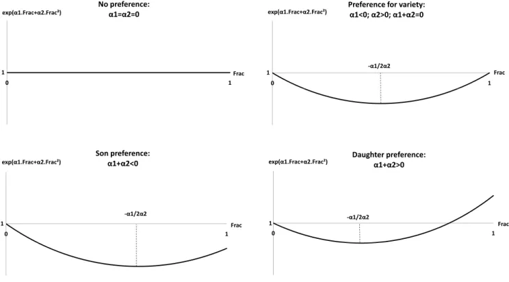
daughter preference. Figure 2 here
We introduce the proportion squared to test for a taste for balance in the gender compo-sition, as illustrated in Figure 2. We plot the multiplier on the baseline hazard as a function of F rac for different values of α1 and α2. On the top left, we plot the trivial case in which
α1 = α2 = 0, meaning that the gender composition of current children has no impact on
subsequent durations. Then, if α1 < 0 and α2 > 0, it implies that the hazard rate is lower for
women having children of each gender. The lowest hazard rate is reached by women having a proportion of boys among their children that is exactly equal to −α1
2α2. Therefore, the longest
duration is predicted to be observed (i) among couples having exactly the same number of boys and girls if α1 + α2 = 0 (graph on the top right) ; (ii) among couples having sons and
daughters, but more sons than daughters, if α1 + α2 < 0 (graph on the bottom left) ; and
20. We introduce some controls to estimate more precisely the baseline hazard for different categories of mothers, thus reducing our standard errors. The magnitude of our estimates is unchanged if we remove the controls.
21. We divide a woman’s individual weight by her number of births. If we do not reweigh the observations, a woman with n births counts n times. So women having more children, meaning women with a taste for large families and older women, are over-represented.
(iii) among couples having sons and daughters, but more daughters than sons, if α1+ α2 > 0
(graph on the bottom right). Our statistic of interest is therefore (α1 + α2).
We define the following classification:22
– No preference: α1 and α2 are not jointly significant.
– Preference for variety: α1 < 0, α2 > 0 and α1+ α2 = 0.
– Preference for boys: α1+ α2 < 0.
– Preference for girls: α1+ α2 > 0.
3.3
Identification assumptions
The main threat to identification is the prevalence of child mortality. In our sample, 15.7% of children died before turning five years old. In this context, when we analyse fertility choices, shall we consider the gender composition of the previous births or the gender com-position of children alive at the time of the decision? There is a trade-off between exogeneity and relevance. The composition that matters to parents is probably among children who survived ; but it is correlated to parents’ choices regarding breastfeeding, nutrition and ca-ring. Indeed, the proportion of sons among survivors could be an outcome of parents’ gender preferences. That is why we consider the proportion among all births. Our strategy is close to an instrumental variable framework: we use the composition among births as an instrument for the composition among survivors, and estimate the reduced form.23
The first key identification assumption is that there is no sex-selective abortion. We believe that it is likely to hold because sex ratio at birth in our sample is equal to 51.2%, which is the ratio observed in Western countries (Brian and Jaisson(2007),Ben-Porath and
22. We do not consider the case α1 > 0, α2 < 0 and α1+ α2 = 0 because we never observe it in our
estimations.
23. Note that we cannot apply a 2SLS procedure because the outcome does not depend linearly on the instrumented variable. As a robustness check, we do the same analysis using the fraction of sons among survivors at the time of conception. We compare the indicator α1+ α2 obtained from this analysis to our
main indicator, and we find a very high correlation between the two (0.97). Our conclusion regarding spatial heterogeneity is unchanged.
Welch (1976) in the US,Jacobsen, Moller, and Mouritsen (1999) in Denmark) and generally considered as the natural level. Moreover, abortions are rare in Africa. Abortion is allowed without restriction only in Tunisia and in South Africa (United Nations,2011b). According to recent estimations including illegal abortions, the number of abortions per 100 live births is 17 in Africa, compared to 34 in Asia and 59 in Europe (Sedgh, Henshaw, Singh, Ahman, & Shah, 2007). Last, sex-selective abortions are even less likely in our context, as obstetric ultrasound is not so common. Today, only 30% of women in cities, and 6% of women in rural areas have access to ultrasound during their pregnancy in Sub-Saharan Africa (Carrera,
2011).
The second identification assumption is that there is no sex-selective child mortality.24
Otherwise, the coefficients in the reduced form capture both the reaction to the death of a child and the « true » impact of gender composition on the next birth. In our sample, boys tend to die more than girls: for 100 girls dying before age five, 111 under-five boys die. This figure is 112 in Sub-Saharan Africa, 105 in North Africa, and it is above 100 in every country.25 Consequently, families with more sons at birth are more likely to have lost one child. If parents intensify fertility after the death of a child, we would observe that families with more sons have shorter birth intervals. So we would tend to underestimate son preference and to overestimate daughter preference everywhere.26 If we find evidence of
son preference, it has to be driven by fertility choices. Sex-selective mortality alone could explain our results only if we conclude that daughter preference prevails. Another question is whether the variation across countries arises mainly from the variation in sex-selective
24. Sex-selective adult mortality could also bias our estimates if parents form beliefs about the survival probability of their sons and daughters at adult age, and take fertility decisions according to these beliefs. However, qualitative evidence provided by demographers do not support the idea that people make such calculations about child loss (Randall & LeGrand,2003).
25. Such a female advantage in mortality is observed in most countries in the world, with the notable exception of India and China. The average world ratio excluding India and China was around 111 during the last decades (United Nations,2011a).
26. Since differential mortality is the lowest in North Africa, it is the region in which son preference would be less underestimated.
mortality. In Section 5.1, we test if our sorting of countries is robust to a potential mortality bias by focusing on parents who lost no child.
Another threat to our strategy is that the prevalence of maternal mortality could lead to sample selection. In particular, if mothers exhibiting specific gender preferences are more likely to die, surviving women would be selected. For instance, suppose that mothers with the strongest son preference shorten birth intervals when they have only girls, increasing their exposure to maternal mortality risk. These women would be under-represented, and our estimate of son preference for surviving mothers would underestimate son preference in the whole population. Conversely, in a daughter preference setting, we would underestimate daughter preference. So selective maternal mortality might lead to underestimating gender preferences.27 In our data, we can get indirect evidence of selective maternal mortality by
looking at the sex ratio of the first born child. In our sample, the ratio is around 0.51 in all countries, but we do find that in some countries, it increases (up to 0.57 in Nigeria), or decreases (down to 0.45 in Sudan) for older women. This is a hint that maternal mortality may be linked to gender preferences in different ways for different countries. We estimate an order of magnitude of the selection bias in Section 5.2.
4
Results
4.1
Comparative descriptive analysis
4.1.1 Heterogeneity over space
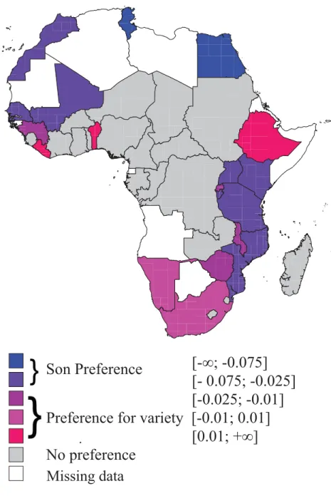
Figure 3 here
Figure 3 maps the magnitude of our indicator of gender preferences (α1+α2) for countries
27. Note that another mechanism could lead to the same bias: if mothers having preferences for sons are more likely to forget first-born girls who died in their first days of life than first-born boys, this sex-selective recall would also lead to an underestimation of gender preferences.
in which α1 and α2 are jointly significant. Otherwise, countries are classified as « no
prefe-rence ».28 We find evidence of son preference in North Africa (Morocco, Tunisia, Egypt),
Mali and Senegal, and also in the Great Lakes region (Burundi, Kenya, Uganda, Mozam-bique, Tanzania). Then, Southern Africa (Namibia and South Africa) is characterized by a preference for variety, and Central Africa (Cameroon, Chad, Congo, Congo DRC, Gabon, Central African Republic) by the absence of revealed gender preferences. In the rest of the continent, countries are divided into no gender preferences (Swaziland, Nigeria, Sierra Leone, Burkina Faso, Ghana, Togo, Niger, Sudan, Zambia, Lesotho and Madagascar, Cote d’Ivoire) and a taste for balance (Guinea, Liberia, Benin, Ethiopia, Rwanda, Malawi and Zimbabwe). No country displays daughter preference.
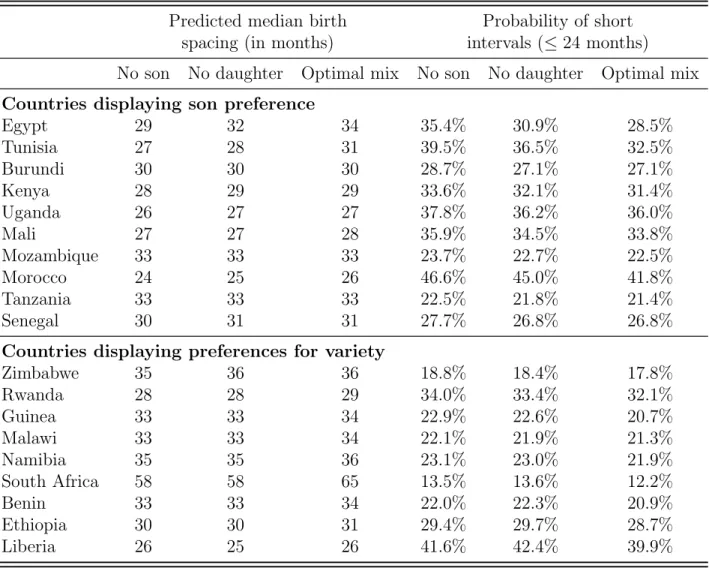
Such a simple sorting fails to give a sense of magnitude. When we predict the size of our coefficients α1 and α2 in a cross-country regression, they increase with the proportion
of Muslims and with the prevalence of contraception.29 Then, we want to estimate by how much gender preferences impact fertility choices. We compute the predicted median birth spacing and the probability of short birth spacing (≤ 24 months)30 for (i) couples with no son ; (ii) couples with no daughter ; and (iii) couples having the optimal mix of sons and daughters.31 Estimations are reported in Table 1 for countries in which we found evidence
of gender preferences ; examining the magnitude is indeed meaningless when the proportion of sons has no significant impact on subsequent births.
Table 1 here
North African countries stand out because they display the largest magnitudes: for ins-tance, in Egypt, having no son is predicted to reduce the median birth spacing by three
28. The classification of countries can also be found in Appendix D in Table A.6.
29. Since contraceptive use is correlated with wealth and total fertility, we also find that the magnitude of preferences increases in wealth and decreases in the number of children per woman.
30. In the Cox model, one can derive an estimate of the survival function bS(t) (Box-Steffensmeier and Jones, 2004). The predicted median birth spacing is τ s.t. bS(τ ) = 0.5 and the probability of short birth spacing is bS(24).
31. The optimal mix is the fraction of sons corresponding to the lowest hazard rate ; it is equal to −2αα1
months as compared to having no daughter, and by five months as compared to the opti-mal mix of sons and daughters. Having no daughter (respectively having the optiopti-mal mix) decreases by 13% (respectively by 20%) the probability to have short birth intervals, compa-red to having no son. There, son preference has a strong impact on fertility patterns. Large magnitudes are also observed in South Africa. When the gender composition is perfectly balanced, couples are predicted to wait seven months more than couples having only boys or only girls. The taste for balance therefore translates into sizeable differences between families. In the rest of Africa, gender preferences have a much weaker impact. Should they display preferences for boys or for variety, all countries exhibit very small differences in predicted birth spacing across our three categories of interest (zero or one month). In case of son pre-ference, having only sons decreases by roughly 4% the probability of short birth spacing as compared to having only daughters.
4.1.2 Heterogeneity over time
To study the evolution of gender preferences over time, we interact our variables of interest with the mother’s birth cohort in the general model:
λ(t) = λ0(t) × exp(λ1.cohort + λ2.cohort2+ ζ1.F racn+ ζ2.F rac2n+ φ1.cohort.F racn+
φ2.cohort2.F racn+ ω1.cohort.F racn2 + ω2.cohort2.F rac2n+ θ.Xn+ κ.C)
We pool all the surveys together, adding a vector of dummies for each country (C) to our main specification. From the estimates, we compute an indicator of cohort-by-cohort gender preference:
[
P ref = bζ1+ bζ2+ bφ1.cohort + bφ2.cohort2+cω1.cohort +cω2.cohort
Considering birth spacing rather than completed fertility allows us to look at contemporary cohorts, because we already have information about the behavior of women born in the 70s and 80s.
Figure 4 here
In Figure 4 we plot [P ref against the birth cohort, together with its 5% confidence intervals, in North Africa and in Sub-Saharan Africa. Our indicator is more and more negative over time in North Africa, meaning that son preference increases. When we break down this trend by country, we find that it is mainly driven by Egypt, especially in the most recent years. As explained in Section 2.1, we have few mothers born after 1970 in Morocco and Tunisia. Before that date, the trend observed in Morocco is similar to the Egyptian one, whereas it is rather flat in Tunisia – if anything, son preference tends to decrease. The reinforcement of son preference in North Africa coincide with fertility transitions, supporting the idea that a reduction in family size exacerbates gender preferences.
In Sub-Saharan Africa, there is not much variation: our indicator is fairly stable across the period. It is slightly increasing during the first decades, but the magnitude of the change is small and imprecisely estimated. For most cohorts, [P ref is not significantly different from zero, so there is no evidence of son preference.
4.2
Key drivers of gender preferences
Now that we have underscored different patterns in Sub-Saharan and in North Africa, one may wonder if socio-economic factors drive some heterogeneity within these areas. In this section, we examine whether preferences vary across categories of women (e.g. educated vs. non-educated, rural vs. urban, matrilineal vs. patrilineal etc.).
4.2.1 Empirical strategy
We introduce interaction terms in our specification:
λ(t) = λ0(t) × exp(γ0.Alter + γ1.F racn+ γ2.F rac2n+ δ1.F racn.Alter + δ2.F rac2n.Alter + θ.Xn+ κ.C)
Where Alter is a dummy equal to 0 if women belong to the reference category, and 1 if they belong to the alternative category. Again, we pool all the surveys together, and we add country and cohort dummies. Then, for each category, we compute our indicator of gender preference (using the notations of the general specification, it corresponds to α1+ α2):
– Reference category: we test if γ1+ γ2 = 0
– Alternative category: we test if γ1+ γ2+ δ1+ δ2 = 0
We can conclude that gender preferences are different between the two categories if δ1 + δ2 is significantly different from 0.
4.2.2 Are religion and family systems shaping preferences?
We start by considering two structural factors that appeared in the literature review as potential drivers of gender preferences: Islamic influence and traditional kinship structure. We can only perform this analysis in Sub-Saharan Africa, because the number of Christians and matrilineal group members is too low in North Africa.
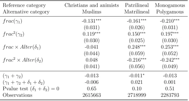
Table 2 here
The first hypothesis we want to test is whether son preference is stronger among Muslims. The depth of Islamic penetration is indeed one way to explain the difference between North and Sub-Saharan African countries. The next question is whether, in Sub-Sub-Saharan Africa, Muslims and other religious groups have different preferences. In the first column of Table 2, we show that Muslims exhibit the same taste for balance as Christians and animists. Coefficients on the interaction terms are not significant, and the indicator of gender preferences is the same in both categories. So religion may play a role at the macro level, by influencing family law, property rights, social norms etc., but in a given institutional setting, it does not seem to drive individual gender preferences.
The second hypothesis is that son preference would prevail in patrilineal ethnic groups, while daughter preference should be observed in matrilineal groups. As shown in Table 2, column 2, this hypothesis is validated: we find that our indicator of gender preferences is negative in patrilineal groups, which means son preference ; whereas it is positive in matrilineal groups, although not significant. Given the small proportion of the sample belonging to a matrilineal group (5.7%), we lack some power to take a definitive stance, but matrilineal groups seem to exhibit daughter preference. In any case, their preferences are significantly different from the ones in patrilineal groups.
When we further split the sample on the median wealth index, we find that our result on kinship structure is driven by relatively rich people. In the poorest half of the sample, couples in patrilineal and matrilineal groups exhibit the same preferences. One interpretation might be that inheritance rules impact gender preferences only when families have enough assets to bequest.
In the third column of Table 2, we test if gender preferences differ across union types: polygamous vs. monogamous. We find preference for variety in monogamous unions, but no evidence of gender preferences in polygamous unions. For them, the coefficients on F rac and F rac2 are very close to zero. Given the caveat that we mentioned in the introduction, this result is not surprising: our unitary model is well-suited to monogamous households, but it is less adequate to describe choices in more complex household structures.
4.2.3 How do preferences relate to modernization?
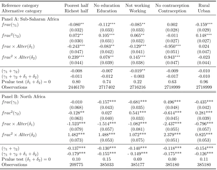
Now, we turn to the modernization hypothesis, and examine individual indicators of develop-ment. Table 3 reports the results for Sub-Saharan Africa in the upper part, and for North Africa in the lower part. More precisely, we compare the poorest half and the richest half of the sample (column 1) ; non-working and working women (column 2) ; women who do and do not use contracep-tion (column 3) ; non-educated and educated women (column 4) ; rural and urban women (column 5) ; each time controlling for all other socioeconomic variables.
Table 3 here
has no impact on the preferred proportion of sons. In the richest half of the sample, coefficients on F rac and F rac2 are both significantly larger in absolute terms than in the poorest half ; but the indicator of preferences for boys vs. girls is the same and reveals preferences for variety. Wealth seems to strengthen the taste for balance, modifying the magnitude, but not the nature of gender preferences. While the same findings hold, to a smaller extent, for education, we find no correlation between gender preferences and the area of residence controlling for education, wealth, employment status and contraceptive use.
The second result is that son preference is very strong for women who do not work, whereas working mothers exhibit preferences for variety. One explanation emphasizes insurance motives for the mother: non-working women are heavily dependent on their husband, and in case of widowhood, on their sons. The prevalence of son preference among non-working mothers also holds in matrilineal groups, suggesting that the insurance motive might prevail over the lineage motive.
Last, the correlation with contraceptive use is in line with expectations. Here, the variable Contraception is equal to one if the woman uses a modern method of contraception at the time of the survey. It does not imply that she was using it during her whole birth history, but it is a good proxy for how much control she has over fertility choices. For women who do not use modern contraceptives, coefficients on F rac and F rac2 are close to zero: the gender composition of previous children does not influence subsequent birth intervals. Either they have no gender preferences, or they lack control over fertility to translate their preferences into actions.
Turning to North Africa, we find evidence of a strong son preference in every category we consider. Here again, the magnitude of preferences is much larger in more ”modern” categories. But the nature of preferences is not substantially affected. The only difference arises with contraception: modern contraceptive users display a significantly stronger son preference than non-users.
4.3
Mechanisms: individual choices or social norms?
The fact that contraceptive use is correlated with revealed preferences raises the question of the mechanisms: how may gender preferences translate into differential spacing behavior? The first
channel we have in mind is a conscious choice made by the couple to bring forward or to delay the next birth in order to reach an ideal gender composition. This requires that couples use birth control methods, be it modern contraceptives or more traditional methods such as varying breastfeeding duration. Another channel deserves attention: there might be social norms surrounding birth spacing practices that produce differential spacing. We think in particular of breastfeeding norms that require children of one gender to be fed longer than others.32 Such norms might reveal gender preferences at the society level. But in an evolutionary perspective, they might also simply reflect the greater biological vulnerability of one gender in the first years of life, and the attempt to reach a balanced sex ratio at reproductive ages.
In Sub-Saharan Africa, the modern contraceptive channel affects a limited fraction of the popu-lation. According to the United Nations, the contraception prevalence in Sub-Saharan Africa was 25% in 2011, and 20% if we focus on modern contraceptive methods. As a comparison, the same fi-gures in Asia were 67% and 61% (United Nations,2012). The limited contraception prevalence may partly explain why we find no differential spacing in most Sub-Saharan countries. Those women who have access to contraception clearly reveal preferences for variety, as shown by Table 3. This result points to a deliberate manipulation of birth intervals. Regarding breastfeeding practices, as already mentioned in the literature review, they do not differ by gender (Chakravarty, 2012; Ga-renne,2003). The equal treatment in breastfeeding might reflect the absence of gender preferences at both individual and social levels.
In North Africa, a larger share of the population uses modern contraceptive methods: the contraception prevalence was 48% in 2011 (United Nations, 2012). As already shown in earlier studies (Yount et al.,2000), contraceptive use depends on the gender composition of earlier births. In our sample, the proportion of women using modern birth control methods is significantly lower (by 1.7 percentage points) after the birth of a girl as compared to a boy. Therefore, the shorter birth intervals observed in families with more daughters are partly generated by different contraceptive choices. This is a first hint that our strategy captures intentional choices. As for breastfeeding
32. Since breastfeeding duration is correlated to the duration of postpartum insusceptibility, such norms may generate systematic differences in birth intervals after the birth of a son vs. a girl (Jayachandran & Kuziemko,2011).
practices, they differ by gender only in Egypt, where we find that boys are significantly more likely than girls to be breastfed longer than 15 months (by two percentage points). This result is in line with Chakravarty (2012) and may originate from individual choices as well as from social norms. We attempt to disentangle both dimensions by decomposing our variable F racn into F racn−1: the proportion of sons among the previous (n−1) births, and Boyn: a dummy indicating whether the nth birth is a boy. Results for North Africa are reported in Table A.7 in Appendix E. The proportion of sons among the previous (n − 1) births has an impact on the duration between births n and (n + 1): we find the same asymmetric U-shape as with F racn. It indicates that parents take into account the gender composition of their whole family. Parents also react to the gender of the latest born: the coefficient on Boysn is negative and significant, which may reflect conscious or less conscious choices. One argument in favor of conscious choices is that the impact of Boysndiffers across birth orders: it is stronger at ranks three and four than at other ranks. Such a pattern is difficult to reconcile with a breastfeeding norm. All in all, we believe that differential spacing should be mainly interpreted as a reflection of conscious, individual choices. Social norms surrounding breastfeeding may also play a role, but the body of evidence seems to indicate that it is limited.
5
Robustness Tests
5.1
Testing the child mortality bias
As mentioned in Section 3.3, we test if sex-selective mortality introduces a bias in our estimates. The idea is to isolate couples who lost at least one child among the previous n births, and to focus on couples who lost no child. If we find evidence of gender preferences for the latter, they cannot be driven by differential mortality, they have to be driven by differential fertility rules. In Table A.8 in Appendix E, we interact F rac and F rac2 with a dummy equal to one if at least one of the previous n children died. As expected, we find that the sex-selective mortality leads us to underestimate the extent of son preference in Africa: our indicator (α1+ α2) is more negative among women who did not lose any children than in the baseline. However, the difference is small, around 10%. Then, we
check if our baseline classification of countries into the « son preference group » and the « preference for variety group » remains valid. In Table A.9 in Appendix E, we find, again, that focusing on couples who lost no child slightly shifts our results towards more son preference. However, (α1+ α2) remains not significantly different from zero in the group classified as « preferences for variety », implying that our findings are robust.
To better understand the magnitude of the bias, we compute the predicted median birth spacing and the probability of stopping for couples who did not lose a child. In absolute values, birth spacing increases by one month, and the probability of stopping by roughly one percentage point, compared to the magnitudes discussed in section 4.1. But in relative terms, the differences across categories remain very stable.
The last test is to look how our sorting of countries is affected by mortality. Going on with same specification, we compute (α1+ α2) among people who lost no child in each country, and compare it to our baseline (α1 + α2). The correlation between both indicators is 0.97. Then, we sort the countries according to each indicator, and the rank correlation is equal to 0.95. In the end, the variation in sex-selective mortality across countries does not seem to drive the variation we observe.33
5.2
Testing the sample selection of mothers
We further deal with a potential selection bias. We run our model on mothers below 40 years old who are less likely to have died or forgotten their earlier-born children.34For this sample of younger mothers, we find that the gender of the first born is exogenous to socioeconomic characteristics, which supports the assumption that the sample is not selected. We find that the correlation between the indicator computed on younger mothers and our baseline indicator is 0.94. Furthermore, the rank correlation between both classifications is 0.88. These strong correlations supports the idea that our results are not driven by differences between countries in maternal mortality or recall bias.
33. Another piece of evidence is given by the low rank correlation (0.16) between our sorting and the sorting of countries on the child mortality ratio between girls and boys.
Last, we checked, as in Table A.9, that our classification of countries into « preference for son » and « preference for variety » remains robust once we restrict our sample to younger mothers.
One limit if this strategy is that maternal mortality affects also young women. In particular, one can fear that when we find no gender preferences in some countries, it might be due to the fact that women having stronger son preference massively died before 40 years old. Let us consider simple back of the envelope calculations to get an order of magnitude of such a downward bias. In countries classified as « no preference », let us assume that there are in fact two groups of women. The first one, accounting for M % of the population, has very strong son preference ; we attribute to them the largest magnitude found in our sample (α1+ α2= −0.17 in Egypt). The second group has no gender preference ; for them, α1 = α2= 0. The scenario that would lead to the most extreme selection bias is that all women having a son preference die, while all women having no preference survive. In this case, M represents the mortality rate. Following our baseline strategy, we would only observe surviving women and compute an indicator of gender preferences equal to 0, whereas the true indicator for the whole population would be around −0.17 × M .35 These countries could therefore reach the lowest magnitude of son preference observed in our sample (α1+ α2= −0.04 in Senegal) if they had a maternal mortality rate at least equal to M = 0.040.17 = 23.5%. It amounts to a lifetime risk of one out of four, a magnitude never reached in Sub-Saharan Africa.36 To conclude, maternal mortality would need to reach unlikely high levels in order to drive our « no preference » results.
5.3
Investigating heterogenous effects across birth ranks
In our model, we pooled all birth ranks together to have more power and to build a single indicator of gender preferences. But some papers in the literature on India have discussed the hete-rogeneous effect of gender preferences across birth ranks. For instance,Jayachandran and Kuziemko
35. Under the technical assumption that the weighted average of our indicator in both groups is a good proxy for the global indicator.
36. By comparison, it is almost ten times higher than the average risk in Sub-Saharan Africa in 2013 (one out of 38), and four times larger than the largest risk (one out of 15 in Chad) (WHO, UNICEF, UNFPA and The World Bank,2014).
(2011) show that the impact of son preference is stronger at higher ranks, when parents get closer to their ideal family size. On the other hand, family size itself may influence preferences:Jayachandran
(2014) finds that son preference increases when families get smaller.
Our strategy might easily be modified to investigate whether the impact of gender preferences differs across birth ranks in Africa.37 We estimate a model similar to Section 4.1.2: we interact our variables of interest with the child’s birth rank, and we compute a rank-by-rank indicator. In Figure A.1, in Appendix E, we plot this indicator together with its 5% confidence intervals in North Africa and in Sub-Saharan Africa. Both graphs display a U-shape, meaning that son preference is the strongest between ranks three and six. At lower and higher ranks, it is much weaker in North Africa, and disappears in Sub-Saharan Africa.
There are three ways to explain this pattern. First, the intensity of gender preferences, for the same couple, may vary across birth orders. It could be low at lowest ranks, because parents still have time for other tries in the future. Then the intensity could increase as time passes by, and parents start worrying about the eventual gender composition of their children. Last, the trend could revert at highest ranks if parents can already count on their eldest children. Second, the ability to control fertility, and hence to translate preferences into differential spacing, may be higher at intermediary ranks. Indeed, at lowest ranks, contraceptive use is less widespread ; and at highest ranks, biological fecundity is lower, which reduces women’s leeway. The last explanation is that gender preferences may be heterogenous across couples depending on the family size. Such a U-shape is consistent with (i) preference for variety in small size families, (ii) son preference in middle size families, and (iii) no preference in large size families.38
These results raise some concern about the implicit assumption in our model that birth orders have a multiplicative effect on the baseline hazard. To remove any doubt, we estimated our model rank by rank, for each country. We retrieved coefficients α1and α2 for each rank, and we computed a weighted average, taking into account the number of observations at each rank. We were thus able to build a new indicator of gender preferences for each country, and we checked that it was
37. In Appendix F, we focus on the situation after the second birth.
38. When we interact F rac and F rac2 with family size instead of birth order (using the subsample of
strongly correlated to our baseline indicator (0.86). The restriction we made on birth order effects in our main specification does not change qualitatively our results.
6
Conclusion
All in all, we find robust evidence that son preference influences fertility patterns in North Africa: people tend to shorten birth spacing and to have additional children as long as they have not had enough sons. This has strong implications for gender inequality: an average girl would be weaned sooner, and would face more competition from her siblings, than an average boy. Moreover, women, as mothers, would put their own lives in jeopardy to ensure that enough sons are born. Policies aiming at reducing women’s reliance on sons, or equalizing the value of sons and daughters to their parents, could weaken the motives for son preference. Ultimately, they could help lengthening birth intervals and improving maternal and child health in North Africa.
We cannot draw the same conclusion for Sub-Saharan Africa: son preference exists in some countries, but it is weak. Overall, fertility behavior is rather consistent with a preference for variety or no preference at all. The impact of gender preferences on fertility patterns is not substantial enough to induce gender inequality. In this context, policies combating son preference will not be enough to curb fertility.
We also showed that differential spacing mainly reflects conscious choices, implemented through contraception, rather than social norms related to breastfeeding. In the likely scenario that some women still have unmet needs for family planning, our results suggest that gender preferences may deepen in the short run. The rise in contraceptive use might exacerbate son preference in North Africa and preference for variety in Sub-Saharan Africa, provided that current contraceptive users reveal preferences that are shared by the whole population. In the longer run, the evolution of gender preferences depends on more structural changes that could impact the nature of preferences, for instance through women empowerment.
The dissimilarity between North Africa and Sub-Saharan Africa can certainly be explained by structural differences in women’s role in society. Yet, we are not claiming that gender inequality
is only an issue in North Africa, but not in Sub-Saharan Africa. There are plenty of mechanisms by which gender preferences prevailing in a society may translate into inequality, beginning with family law and property rights. On many dimensions, it might be argued that women do have a subordinate status in Sub-Saharan Africa. Anderson and Ray (2010) show that, in this region, there are « missing women », too. But contrary to India and China, they are in majority of adult age ; HIV/AIDS and maternal deaths are the two main sources of female excess mortality. The discrimination against women would appear later in life: at puberty? At marriage? At motherhood? At widowhood? Understanding when and why remains an open question.
References
Abrevaya, J. (2009). Are there missing girls in the united states? evidence from birth data. American Economic Journal: Applied Economics, 1(2), 1-34.
Agarwal, B. (1994). A field of one’s own: Gender and land rights in south asia. Cambridge: Cambridge University Press.
Anderson, S., & Ray, D. (2010). Missing women: Age and diseases. Review of Economic Studies, 77 , 1262-1300.
Arnold, F. (1992). Sex preference and its demographic and health implications. International Family Planning Perspectives, 18 , 93-101.
Arnold, F., Choe, M., & Roy., T. (1998). Son preference, the family-building process and child mortality in india. Population Studies, 52(3), 301–315.
Arnold, F., & Liu, Z. (1986). Sex preference, fertility, and family planning in china. Popu-lation and Development Review , 12 , 221-246.
Barbar, J., & Axinn, W. (2004). New ideals and fertility limitation: The role of mass media. Journal of Marriage and Family, 66 , 1180-1200.
Basu, A. (1999). Fertility decline and increasing gender imbalance in india, including a possible south indian turnaround. Development and Change, 30 , 237-263.
Basu, D., & Jong, R. de. (2010). Son targeting fertility behavior: Some consequences and determinants. Demography, 472 , 521-536.
Ben-Porath, Y., & Welch, F. (1976). Do sex preferences really matter? Quarterly Journal of Economics, 90 , 285-307.
Bhat, P., & Zavier, A. (2003). Fertility decline and gender bias in northern india. Demogra-phy, 40 , 637-657.
Brian, E., & Jaisson, M. (2007). Le sexisme de la premi`ere heure. hasard et sociologie. Raisons d’agir, Paris.
Carrera, J. (2011). Obsetric ultrasounds in africa: Is it necessary to promote their appropriate use? Donald School Journal of Ultrasound in Obsetrics and Gynaecology, 5 , 289-296. Chakravarty, A. (2012). Child health and policy implications: Three essays on india and
africa. Doctoral thesis, UCL.
Clark, S. (2000). Son preference and sex composition of children: Evidence from india. Demography, 37(1), 95-108.
Cohen, B. (1998). The emerging fertility transition in sub-saharan africa. World Develop-ment , 26(8), 1431-1461.
Conde-Agudelo, A., & Belizan, J. (2000). Maternal morbidity and mortality associated with interpregnancy interval: Cross sectional study. British Medical Journal , 321(7271), 1255-1259.
Conde-Agudelo, A., Rosas-Bermudez, A., & Kafury-Goeta, A. (2006). Birth spacing and risk of adverse perinatal outcomes : A meta-analysis. The Journal of the American Medical Association, 295(15), 1809-1823.
Cox, D. R. (1972). Regression models and life-tables (with discussion). Journal of the Royal Statistical Society Series B , 34 , 187-220.
Das Gupta, M. (1987). Selective discrimination against female children in rural punjab, india. Population and Development Review , 13 , 77-100.
Das Gupta, M., Zhenghua, J., Bohua, L., Zhenming, X., Chung, W., & Hwa-Ok, B. (2003). Why is son preference so persistent in east and south asia? a cross-country study of china, india and the republic of korea. The Journal of Development Studies, 40(2), 153-187.
Deaton, A. (1987). Allocation of goods within the household: Adults, children, and gender. Research Program in Development Studies, Princeton University, and LSMS, World Bank .
Edlund, L., & Lee, C. (2013). Son preference, sex selection and economic development: The case of south korea. NBER Working Paper .
Flato, M., & Kotsadam, A. (2014). Droughts and gender bias in infant mortality in sub-saharan africa. WP University of Oslo.
Friedman, J., & Schady, N. (2012). How many infants likely died in africa as a result of the 2008-09 global financial crisis? WP World Bank Policy Research.
Fuse, K. (2008). Gender preferences for children: a multi-country study. Dissertation, Graduate School of The Ohio State University.
Gangadharan, L., & Maitra, P. (2003). Testing for son preference in south africa. Journal of African Economies, 12(3), 371-416.
Garenne, M. (2003). Sex differences in health indicators among children in african dhs. Journal of Biosocial Science, 35(4), 601-614.
Ghilagaber, G., & Gyimah, S. O. (2004). A family of flexible parametric duration functions and their applications to modelling child-spacing in sub-saharan africa. PSC Discussion Papers Series, 18(1).
Gray, J. P. (1998). Ethnographic atlas codebook. World Culture, 10(1), 86-136.
Hatlebakk, M. (2012). Son-preference, number of children, education and occupational choice in rural nepal. CMI Working Paper .
Plan-ning, 26(6), 325-337.
Jacobsen, R., Moller, H., & Mouritsen, A. (1999). Natural variation in the human sex ratio. Human Reproduction, 14(12), 3120-3125.
Jayachandran, S. (2014). Fertility decline and missing women. NBER Working Papers. Jayachandran, S., & Kuziemko, I. (2011). Why do mothers breastfeed girls less than boys?
evidence and implications for child health in india. The Quarterly Journal of Econo-mics, 126 , 1485-1538.
Jensen, R. (2005). Equal treatment, unequal outcomes? generating sex inequality through fertility behavior. Unpublished document. JFK School of Government, Harvard Uni-versity..
Klasen, S. (1996). Nutrition, health and mortality in sub-saharan africa: Is there a gender bias? Journal of Development Studies, 32 , 913-943.
Koolwal, G. (2007). Son preference and child labor in nepal: The household impact of sending girls to work. World Development , 35(5), 881-903.
Lambert, S., & Rossi, P. (2014). Sons as widowhood insurance: Evidence from senegal. PSE Working Papers.
Larsen, U., Chung, W., & Gupta, M. D. (1998). Fertility and son preference in korea. Population Studies, 52 , 317-325.
Lesthaeghe, R. (1989). Reproduction and social organization in sub-saharan africa. Berkeley: University of California Press.
Leung, S. (1988). On tests for sex preferences. Journal of Population Economics, 1 , 95-114. Leung, S. (1991). A stochastic dynamic analysis of parental sex preferences and fertility.
Quarterly Journal of Economics, 106(4), 1063-1088.
Mace, R., & Sear, R. (1997). Birth interval and the sex of children in a traditional african population: An evolutionary analysis. Journal of Biosocial Science, 29(4), 499-507. Milazzo, A. (2014). Son preference, fertility and family structure: Evidence from reproductive
behavior among nigerian women. WP World Bank Policy Research.
Murdock, G. P. (1959). Africa: Its peoples and their culture history. New York: McGraw-Hill Book Company.
Pande, R. (2003). Selective gender differentials in childhood nutrition and immunization in rural india: The role of siblings. Demography, 40(3), 395-418.
Pong, S. (1994). Sex preference and fertility in peninsular malaysia. Studies in Family Planning, 25(3), 137-148.
Poston, D. (2002). Son preference and fertility in china. Journal of Biosocial Science, 34 , 333-347.
Rahman, M., & DaVanzo., J. (1993). Gender preference and birth spacing in matlab, bangladesh. Demography, 30(3), 315-332.
Rajan, S., Sudha, S., & Mohanachandran, P. (2000). Fertility decline and worsening gender bias in india: Is kerala no longer an exception? Development and Change, 31 , 1085-1092.
Randall, S., & LeGrand, T. (2003). Reproductive strategies and decisions in senegal: the role of child mortality. Population, 58(6), 687-715.
Rose, E. (1999). Consumption smoothing and excess female mortality in rural india. Review of Economics and Statistics, 81 (1), 41-49.
Sedgh, G., Henshaw, S., Singh, S., Ahman, E., & Shah, I. (2007). Induced abortion: Esti-mated rates and trends worldwide. The Lancet , 370 , 1338-1345.
Sen, A. (1990). More than 100 million women are missing. New York Review of Books. Sen, A. (2001). The many faces of gender inequality. Frontline, 18(22).
Tsay, W., & Chu, C. C. (2005). The pattern of birth spacing during taiwan’s demographic transition. Journal of Population Economics, 18 , 323.
Tu, P. (1991). Birth spacing patterns and correlates in shaanxi, china. Studies in Family Planning, 22(4), 255-263.