HAL Id: hal-00302884
https://hal.archives-ouvertes.fr/hal-00302884
Submitted on 19 Jul 2007
HAL is a multi-disciplinary open access
archive for the deposit and dissemination of
sci-entific research documents, whether they are
pub-lished or not. The documents may come from
teaching and research institutions in France or
abroad, or from public or private research centers.
L’archive ouverte pluridisciplinaire HAL, est
destinée au dépôt et à la diffusion de documents
scientifiques de niveau recherche, publiés ou non,
émanant des établissements d’enseignement et de
recherche français ou étrangers, des laboratoires
publics ou privés.
grassland ecosystem to finite-amplitude perturbations
M. Mu, Biao Wang
To cite this version:
M. Mu, Biao Wang. Nonlinear instability and sensitivity of a theoretical grassland ecosystem to
finite-amplitude perturbations. Nonlinear Processes in Geophysics, European Geosciences Union (EGU),
2007, 14 (4), pp.409-423. �hal-00302884�
www.nonlin-processes-geophys.net/14/409/2007/ © Author(s) 2007. This work is licensed
under a Creative Commons License.
Nonlinear Processes
in Geophysics
Nonlinear instability and sensitivity of a theoretical grassland
ecosystem to finite-amplitude perturbations
M. Mu1and B. Wang1,2
1LASG, Institute of Atmospheric Physics, Chinese Academy of Sciences, Beijing 100029, China 2College of Math. and Information Science, Henan Univ., Kaifeng 475001, China
Received: 12 October 2006 – Revised: 29 June 2007 – Accepted: 6 July 2007 – Published: 19 July 2007
Abstract. Within a theoretical model context, the sensitivity
and instability of the grassland ecosystem to finite-amplitude perturbations are studied. A new approach of conditional nonlinear optimal perturbations (CNOPs) is adopted to inves-tigate this nonlinear problem. It is shown that the linearly sta-ble grassland (desert) states can be nonlinearly unstasta-ble with finite-amplitude initial perturbations, which represent the hu-man activities and natural factors on the ecosystem. When the moisture index is between the two bifurcation points, a large enough finite amplitude perturbation can induce a tran-sition from the grassland (desert) state to the desert (grass-land) state. The thresholds of such transition along the bifur-cation diagram of the moisture index are also given by the CNOPs approach. The results also support the viewpoint of Zeng et al., whose emphasis is on the shading effect of wilted grass on the grassland ecosystem. Comparisons between the results obtained by approach of CNOPs and linear singular vectors are made, which demonstrates that CNOPs is a use-ful tool to explore the nonlinear features of the ecosystem.
1 Introduction
In semi-arid areas, it is of importance to study the biosphere-geosphere interaction and ecosystem transition. The ecosys-tem equilibria could coexist with favorable climate condi-tion (Klausmeier, 1999). The transicondi-tion between different ecosystem equilibria often occurs due to the change of cli-mate conditions (Brovkin et al., 1998). UNEP (1992) showed that transitions between desert and humid climates occur for a ratio of precipitation to potential evapotranspiration, i.e.,
µ, the “moisture index”, from 0.2 to 0.5. Over this range,
the sunlight and temperature are usually sufficient to sup-port grasses, but the irregularity and the lack of precipitation
Correspondence to: M. Mu
make the soil water budget become the most important factor in influencing the growth of vegetation. For this reason, the existence of vegetation in such region is fragile. Claussen et al. (1999) and Zeng et al. (2000, 2002) studied the transi-tions in the Sahel/Sahara region with CLIMBER-2 and Zeng-Neelin models respectively. To study the phenomenon of the coexistence of grassland and desert, and to investigate whether and how human activities and natural factors in-duce the transitions between them, Zeng et al. (1994, 2004) and Zeng and Zeng (1996) established simple prognostic models with two- and three-variable grassland ecosystem. Both of the models demonstrate successfully the coexistence of grassland and desert. There are quite a few ecosystem models in which there exist multiple equilibrium regimes. Among these models, the models established by Zeng and his colleagues are remarkable, since they are mathematically simple, possess essential processes, and have shown poten-tial applicability in theoretical research and in deepening the understanding of the mechanism of the ecosystem evolution. Using linear stability analysis approach and the three-variable model, Zeng et al. (2004) find that the model has multiple equilibrium states for certain parameter values and there exist two bifurcation points: µ1and µ2. Figure 1 shows
the equilibrium states under different values of the moisture index µ. When µ<µ1, there is only one linearly stable desert
equilibrium state (DES, solid line). For µ1<µ<µ2, there
exist one linearly unstable grassland equilibrium state (GES, dashed line), and two linearly stable states, one is GES and another is DES (solid lines). When µ>µ2, there are one
lin-early stable GES (solid line) and one linlin-early unstable DES (dashed line). In linear analysis, the definition of linearly stable equilibrium state is as follows. For the linearized sys-tem around an equilibrium state, if there is a normal-mode perturbation growing exponentially, the equilibrium state is called linearly unstable. Otherwise, it is referred as lin-early stable. But this model is a nonlinear ecosystem, to study the effects of human activities and natural variations
0.2 0.25 0.3 0.35 0.4 0.45 0.5 −0.2 0 0.2 0.4 0.6 0.8 1 1.2 1.4 1.6
µ(moisture index)
x (living grass)
µ 1 µ2 A (µ=0.32)(a)
D (µ=0.38) B (µ=0.32) C (µ=0.30) 0.2 0.25 0.3 0.35 0.4 0.45 0.5 0.2 0.4 0.6 0.8 1 1.2 1.4 1.6 µ(moisture index) y (soil wetness) µ 1 µ2 (b) A (µ=0.32) D (µ=0.38) B (µ=0.32) C (µ=0.30) 0.2 0.25 0.3 0.35 0.4 0.45 0.5 −0.2 0 0.2 0.4 0.6 0.8 1 1.2 1.4 µ(moisture index) z (wilted grass) µ1 µ 2 A (µ=0.32) (c) D (µ=0.38) B (µ=0.32) C (µ=0.30)Fig. 1. The equilibrium states vs. the moisture index µ (a) living
grass ¯x, (b) soil wetness ¯y, and (c) wilted grass ¯z . The bifurcation points are indicated as µ1and µ2. Solid and dashed lines refer to linearly stable and unstable equilibrium states, respectively.
on the ecosystem, we should consider its nonlinear instabil-ity and sensitivinstabil-ity. In this paper, we use the model of Zeng et al. (2004) to study whether and how transitions between the different equilibrium states occur and the sensitivity and sta-bility of the model to finite amplitude initial perturbations, which represent the human activities and natural factors on the ecosystem.
To deal with this nonlinear problem, a new approach of conditional nonlinear optimal perturbations (CNOPs) is adopted. CNOPs is proposed by Mu et al. (2003a), and has been utilized to study ENSO by Mu et al. (2003b, 2007a, b) and Duan et al. (2004, 2006), and the ocean’s thermo-haline circulation problems by Mu et al.(2004) and Sun et al. (2005). Their work shows that CNOPs is a useful tool in the studies of predictability, sensitivity and nonlinear stabil-ity analysis.
In the next section, the model and the method of CNOPs are described. Section 3 is concerned with the instability and sensitivity analysis of the grassland ecosystem by us-ing CNOPs and linear sus-ingular vectors methods. The final section is the conclusion and discussion.
2 The model and the CNOPs
2.1 Model
We consider the dynamical ecosystem model of Zeng et al. (2004). This model considers a single vertical column of soil and one species of grass, and has three dimension-less state variables: x, the mass density of living grass, y, the available soil wetness, and z, the mass density of wilted grass, where ˜x=xx∗, ˜y=yy∗, and ˜z=zz∗with ( ˜x, ˜y, ˜z) and
(x∗, y∗, z∗) being dimensional variables and corresponding characteristic values. The model is as following
d ˜x dt = x∗dx dt = F1= G(x, y) − D(x, y) − C(x), (1a) d ˜y dt= y∗dy
dt =F2=P −Es(x, y, z)−Er(x, y)−R(x, y, z), (1b) d ˜z
dt = z∗dz
dt = F3= Gz(x, y) − Dz(z) − Cz(x, y, z), (1c)
where terms G, D, and C are the growth (photosynthesis sub-tracts plant respiration), wilting, and consumption (grazing) of the living leaves, P is the atmospheric precipitation (sys-tem input), Es is the evaporation from the soil surface, Er is the transpiration, and R is runoff, Gz, Dz, and Czare the accumulation, decomposition and consumption of the wilted grass. Readers can refer to Appendix A or Zeng et al. (2004) for detailed description of the model. The parameters and coefficients in model (1) are given in Table A1. It is clear from Appendix that Eq. (1) is a nonlinear model. Also note that in Eq. (1) time is a dimensional variable (units: year).
In this paper, we fix the two parameters: κ1=0.3, which
is the correction due to the non-opaque cover of the liv-ing grass for the diffusive radiation, and ϕrs=0.7 (see Ap-pendix), which stands for the ratio of potential transpiration to potential evaporation, and let the soil moisture index µ be the control parameter. In the following, we need the exact values of the bifurcation points, which is not given in Zeng et al. (2004). Hence, we repeat their work and find the bi-furcation points are µ1=0.3104 and µ2=0.3745, which are
plotted in Fig. 1.
2.2 Conditional nonlinear optimal perturbations
Now let us give a brief introduction to the method of CNOPs. Through this paper, variables with a bar stand for unperturbed ones, and primed variables denote the perturba-tions. Let the vectors ¯U0=( ¯x0, ¯y0, ¯z0) be the initial values,
u′0=(x0′, y′0, z′0) be the initial perturbations to ¯U0. The
vec-tors ¯U(t )=( ¯x(t ), ¯y(t ), ¯z(t )) and ¯U(t )+u′(t ) are the solutions
of model (1) with initial values ¯U0and ¯U0+u′0, i.e., ¯
U(t ) = Mt( ¯U0), U(t ) + u¯ ′(t ) = Mt( ¯U0+ u′0) (2)
where the nonlinear propagator Mt is de-fined as the evolution operator of model (1),
u′(t )=(x′(t ), y′(t ), z′(t )) is the nonlinear evolution of u′0, and (x(t ), y(t ), z(t ))=( ¯x+x′(t ), ¯y+y′(t ), ¯z+z′(t )).
For a chosen norm k · k measuring ¯U(t ), the initial
per-turbation u′0δis called the conditional nonlinear optimal per-turbation with constraint condition, ku′0k≤δ and T >0, if and
only if J (u′0δ) = max ku′ 0k≤δ J (u′0), (3) where J (u′0) = kMT( ¯U0+ u′0) − MT( ¯U0)k, (4)
and δ>0 is a predesignated constant which represents the magnitude of initial perturbations.
The CNOP is the initial perturbation whose nonlinear evo-lution attains the maximal value of the cost function J , which is constructed according to the problems of interests at a specified time T with physical constraint conditions; in this sense it is called “optimal”. The CNOP can be regarded as the most nonlinearly unstable (or most sensitive) initial per-turbation superposed on the basic state. Under a constraint condition, the CNOP drives the ecosystem drifting the far-thest away from the basic state at the specified time. In gen-eral, it is difficult to obtain an analytical expression of the CNOP, so we look for the numerical solution by solving a constraint nonlinear optimization problem.
In this paper, the norm
ku′0k = q (x0′)2+ (y′ 0)2+ (z ′ 0)2 (5) is adopted.
Using a fourth-order-Runge-Kutta method with a time step dt=0.1, and integrating the model (1) with the ini-tial values ¯U0and ¯U0+u′0 to time T , perturbation solutions (x′(t ), y′(t ), z′(t )) are obtained numerically. The Spectral
Projected Gradient (SPG) method is applied to obtain the CNOP numerically. A detailed description of the algorithms can be found in Birgin et al. (2000, 2001, 2003).
3 Nonlinear stability and sensitivity analysis
It follows from above section that bifurcation points µ1and µ2 separate the parameter interval into three parts: µ<µ1, µ1<µ<µ2 and µ>µ2. In this section, we investigate the
nonlinear stability and instability of the equilibrium states in these three intervals respectively. To this end, we compute the CNOPs and investigate their nonlinear evolutions. Two problems are addressed: (i) whether a linearly stable grass-land (desert) state could be nonlinearly unstable, i.e., there exists at least a finite-amplitude perturbation which induces a transition from grassland (desert) to desert (grassland) state; and (ii) the role of moisture index in the sensitivity and insta-bility of the ecosystem.
3.1 Nonlinear instability and evolution of finite-amplitude perturbations represented by CNOPs
Firstly, our attention is paid to the bifurcation interval
(µ1, µ2). In this case, GESs represented by the dashed
line in Fig. 1 are linearly unstable, so we only need to in-vestigate the linearly stable GESs and DESs (solid lines in Fig. 1). To this purpose, a number of values of µ in
(µ1, µ2) and the corresponding GESs and DESs are
cho-sen to calculate their CNOPs. Here we show the results of GES A (Fig. 1): ¯x=0.638139, ¯y=0.669322, ¯z=0.649726
with δ=0.2, 0.4, 0.5 and 0.6; and the results of DES B:
¯
x=0.0, ¯y=0.382380, ¯z=0.0 with δ=0.2, 0.3 and 0.5. In the
calculation, µ=0.32, T =10.0, i.e. 10 years, is the time in-terval, over which CNOPs are derived, and the time step
dt =0.1, which is 0.1 year.
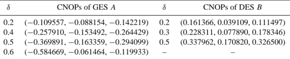
With the Spectral Projected Gradient (SPG) method, we obtain the CNOPs of these two basic states. The components of CNOPs are given in Table 1.
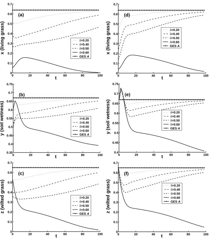
Then we investigate the nonlinear evolution of the ecosys-tem by integrating model (1) with the CNOPs plus GES A as initial values. In Figs. 2a–c, the three components of the non-linear evolutions of the ecosystem are represented by curves. For the convenience of illustrating the results, the compo-nents of GES A are also plotted, which are straight lines there. In cases of δ=0.2, 0.4 and 0.5, the CNOPs causes the ecosystem to evolve to GES A. The three variables recover to GES A shortly after being disturbed with a small-amplitude CNOP (δ=0.2). It takes much longer time to recover to GES
A for a larger amplitude CNOP (δ=0.5). For δ=0.6, the
Table 1. CNOPs of GES A and DES B (µ=0.32, T =10.0).
δ CNOPs of GES A δ CNOPs of DES B
0.2 (−0.109557, −0.088154, −0.142219) 0.2 (0.161366, 0.039109, 0.111497) 0.4 (−0.257910, −0.153492, −0.264429) 0.3 (0.228311, 0.077890, 0.178346) 0.5 (−0.369891, −0.163359, −0.294099) 0.5 (0.337962, 0.170820, 0.326500)
0.6 (−0.584669, −0.061464, −0.119933) – –
the example of δ=0.6 to give the physical mechanism of the evolution of ecosystem. Figure 2a–c shows that in this case, the initial values satisfy that dx/dt and dy/dt are positive and dz/dt is negative, so the mass density of living grass x and the soil wetness y increase, and the mass density of dead grass z decrease at first. But x is very small and z decreases rapidly for about ten years, it causes the evaporation of the soil water increasing, after increasing for about three years,
y decreases suddenly. It induces the living grass lose its
liv-ing condition and viability, after increasliv-ing a little for about twelve years, x decrease in the end, and the grassland ecosys-tem becomes a DES irreversibly. When δ=0.2, 0.3 and 0.5, the physical mechanism of the ecosystem can also be given to explain why the mass density of living grass decreases for few years at first, and increases to be GES in the end. Here, details are omitted.
Zeng et al. (2004) pointed that, in the ecosystem with soil surface shaded by plenty of wilted grass, soil evaporation is reduced significantly, and hence the soil wetness is con-served. Thus, this shading is important for the occurrence of vegetation in semi-arid areas. Our results also support their point of view. At first sight the initial perturbation
u′1=(x0′, y′0, z′0)=(−δ, 0, 0), which decreases the living grass
as much as possible, is likely to induce a larger impact than other initial perturbations for GES. But Table 1 shows that the components of CNOPs of GES A are all negative. For
δ=0.2, 0.4, 0.5 and 0.6, we integrate model (1) to obtain the
nonlinear evolutions of the ecosystem with initial state being
u′1plus GES A, the results are plotted in Figs. 2d–f. Com-paring Figs. 2a–c with Figs. 2d–f we find that the evolutions of CNOPs plus GES A are faster than that of u′1plus GES A. For example, when δ=0.6, the CNOP causes GES A evolve to DES B much faster than the initial perturbation u′1. The negativeness of component z′0of CNOPs in Table 1 for GES
A does show the important shading effect of wilted grass,
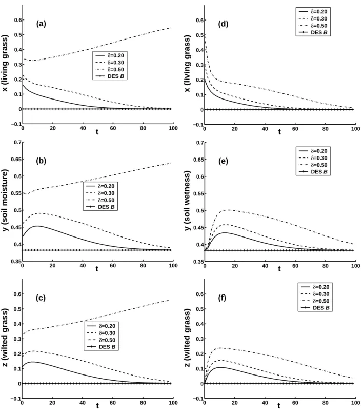
which accords with the opinions of Zeng et al. (2004). For DES B, the nonlinear evolutions of ecosystem with CNOPs plus DES B as the initial conditions are plotted in Figs. 3a–c. In cases of δ=0.2 and 0.3, the ecosystems are at-tracted back to DES B. The three variables recover to DES B shortly after being disturbed with a small amplitude CNOP (δ=0.2). It takes longer time to recover to DES B with a larger amplitude CNOP (δ=0.3). For δ=0.5, the ecosystem evolves to GES A, and the physical mechanism of this
tran-sition is as follows. In Figs. 3a–c, when δ=0.5, the initial values satisfy that dx/dt and dy/dt are negative and dz/dt is positive, thus at first stage, the mass density of living grass
x and the soil wetness y decrease, and the mass density of
dead grass z increases. The increase of z causes a reduction of evaporation of the soil water, and the decrease of x causes a reduction of consumption of the soil water. Therefore, after decreasing for about four years, y increases suddenly. Be-sides, the initial value of x is quite large, so after decreas-ing for about seven years, x increases, and the ecosystem evolves to the grassland state in the end. The physical mech-anism with δ=0.2 and 0.3 can also be given to explain why the ecosystem recovers back to DES in the end. For simplic-ity, it is omitted here.
It is demonstrated above that for GES A the shading ef-fect of dead leaves plays an important roles in the evolu-tions of the ecosystems. This is also true for DES B. With-out careful consideration, one might think that the more grass planted, the larger the positive impacts are. But the dead leaves component z′0of the CNOPs for DES B are all positive (Table 1), which show that the initial perturbation
u′1=(x0′, y0′, z′0)=(δ, 0, 0) does not induce the largest impact
on the ecosystem, but CNOPs does. Taking δ=0.2, 0.3 and 0.5, and integrating model (1), we get the nonlinear evolu-tions of ecosystem with u′1plus DES B as initial conditions. The results are shown in Figs. 3d–f. In contrast to the case of CNOPs, evolutions of u′1plus DES B all recover back to DES B. The larger δ is, the more time the ecosystem will need to recover back to DES B. This tells us that CNOPs is the optimal initial perturbations. In Table 1, the components of CNOPs of DES B are all positive, and z/x approaches 1 as the amplitude becomes larger. And at the same time, y/x increases as the amplitude increases. This shows the impor-tance of shading of wilted grass and the effect of irrigating. This suggests that for DES, we should consider the general effect of all factors and adopt comprehensive actions, such as planting grass, irrigating measurably and shading the ground with dead leaves etc. at the same time to improve the ecosys-tem. This also supports the conclusions of Zeng et al. (2004, 2005a, b).
The above results demonstrate that, in case of µ=0.32, al-though GES A (DES B) is linearly stable, it is nonlinearly unstable, which means that it can be driven to DES B (GES
0 20 40 60 80 100 0 0.1 0.2 0.3 0.4 0.5 0.6 0.7 t x (living grass) δ=0.20 δ=0.40 δ=0.50 δ=0.60 GES A (a) 0 20 40 60 80 100 0 0.1 0.2 0.3 0.4 0.5 0.6 0.7 t x (living grass) δ=0.20 δ=0.40 δ=0.50 δ=0.60 GES A (d) 0 20 40 60 80 100 0.35 0.4 0.45 0.5 0.55 0.6 0.65 0.7 0.75 t y (soil wetness) δ=0.20 δ=0.40 δ=0.50 δ=0.60 GES A (b) 0 20 40 60 80 100 0.4 0.45 0.5 0.55 0.6 0.65 0.7 0.75 t y (soil wetness) δ=0.20 δ=0.40 δ=0.50 δ=0.60 GES A (e) 0 20 40 60 80 100 0 0.1 0.2 0.3 0.4 0.5 0.6 0.7 t z (wilted grass) δ=0.20 δ=0.40 δ=0.50 δ=0.60 GES A (c) 0 20 40 60 80 100 0 0.1 0.2 0.3 0.4 0.5 0.6 0.7 t z (wilted grass) δ=0.20 δ=0.40 δ=0.50 δ=0.60 GES A (f)
Fig. 2. The 100-year nonlinear evolutions of the ecosystem, with GES A plus CNOPs and perturbations u′1=(−δ, 0, 0) as initial conditions.
(a), (b) and (c): CNOPs case; (d), (e) and (f): u′1case.
With CNOPs being initial perturbation, the behaviour of the evolution of the ecosystem also suggests that we should look at a long-term behaviour rather than a short-term one for the ecosystem. For other values of µ in (µ1, µ2), we also find
out CNOPs and investigate the nonlinear evolutions of the ecosystem with CNOPs superposed on the basic state. Al-though there are quantitative differences, the essential char-acteristics are the same; the components of CNOPs are all
0 20 40 60 80 100 −0.1 0 0.1 0.2 0.3 0.4 0.5 0.6 t x (living grass) δ=0.20 δ=0.30 δ=0.50 DES B (a) 0 20 40 60 80 100 −0.1 0 0.1 0.2 0.3 0.4 0.5 0.6 t x (living grass) δ=0.20 δ=0.30 δ=0.50 DES B (d) 0 20 40 60 80 100 0.35 0.4 0.45 0.5 0.55 0.6 0.65 0.7 t y (soil moisture) δ=0.20 δ=0.30 δ=0.50 DES B (b) 0 20 40 60 80 100 0.35 0.4 0.45 0.5 0.55 0.6 0.65 0.7 t y (soil wetness) δ=0.20 δ=0.30 δ=0.50 DES B (e) 0 20 40 60 80 100 −0.1 0 0.1 0.2 0.3 0.4 0.5 0.6 t z (wilted grass) δ=0.20 δ=0.30 δ=0.50 DES B (c) 0 20 40 60 80 100 −0.1 0 0.1 0.2 0.3 0.4 0.5 0.6 t z (wilted grass) δ=0.20 δ=0.30 δ=0.50 DES B (f)
Fig. 3. The same as Fig. 2, but with DES B plus CNOPs and perturbations u′1=(δ, 0, 0) as initial conditions. (a), (b) and (c): CNOPs case;
(d), (e) and (f): u′1case.
negative (positive) perturbations with three variables for GES (DES); when δ is large enough, the CNOPs will induce tran-sitions from GES (DES) to DES (GES). For simplicity, de-tails are omitted.
In case of µ<µ1, there are only DESs, and we choose
them as the basic states with different parameter values of
µ<µ1. We take the case of µ=0.30 as an example to
0 20 40 60 80 100 0 0.05 0.1 0.15 0.2 0.25 0.3 0.35 t x (living grass) δ=0.2 δ=0.3 δ=0.4 (a) 0 20 40 60 80 100 −0.2 0 0.2 0.4 0.6 0.8 1 1.2 t x (living grass) δ=0.8 δ=1.0 δ=1.04795 δ=1.1 δ=1.2 (d) 0 20 40 60 80 100 0.35 0.4 0.45 0.5 t y (soil wetness) δ=0.2 δ=0.3 δ=0.4 (b) 0 20 40 60 80 100 0.4 0.5 0.6 0.7 0.8 0.9 1 1.1 t y (soil wetness) δ=0.8 δ=1.0 δ=1.04795 δ=1.1 δ=1.2 (e) 0 20 40 60 80 100 0 0.05 0.1 0.15 0.2 0.25 0.3 0.35 t z (wilted grass) δ=0.2 δ=0.3 δ=0.4 (c) 0 20 40 60 80 100 −0.2 0 0.2 0.4 0.6 0.8 1 1.2 t z (wilted grass) δ=0.8 δ=1.0 δ=1.04795 δ=1.1 δ=1.2 (f)
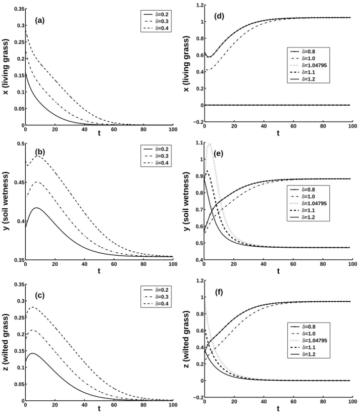
Fig. 4. The 100-year nonlinear evolutions of the ecosystem, left (right) column: CNOPs plus DES C (GES D) as initial conditions, µ=0.30
(µ=0.38).
nonlinear evolutions of the ecosystem with CNOPs plus DES
C: ¯x=0.0, ¯y=0.353949, ¯z=0.0 as the initial conditions. The
amplitude δ=0.2, 0.3 and 0.4, and T =10.0 years. The
com-ponents of CNOPs are all positive and are given in Table 2. The results show that all the CNOPs cause the ecosystem to recover back to DES C in this case. The larger the amplitude
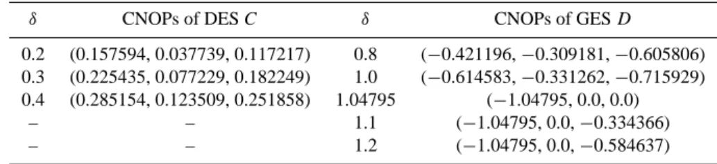
Table 2. CNOPs of DES C (µ=0.30, T = 10.0) and GES D (µ=0.38, T =20.0).
δ CNOPs of DES C δ CNOPs of GES D
0.2 (0.157594, 0.037739, 0.117217) 0.8 (−0.421196, −0.309181, −0.605806)
0.3 (0.225435, 0.077229, 0.182249) 1.0 (−0.614583, −0.331262, −0.715929)
0.4 (0.285154, 0.123509, 0.251858) 1.04795 (−1.04795, 0.0, 0.0)
– – 1.1 (−1.04795, 0.0, −0.334366)
– – 1.2 (−1.04795, 0.0, −0.584637)
Table 3. CNOPs of GES (δ=0.6) and DES (δ=0.3), from µ=0.32 to 0.36, and T =10.0.
µ CNOPs of GESs CNOPs of DESs
0.32 (−0.584669, −0.061464, −0.119933) (0.228311, 0.077890, 0.178346) 0.33 (−0.417145, −0.209649, −0.376878) (0.229372, 0.077854, 0.176995) 0.34 (−0.359608, −0.235794, −0.418430) (0.230118, 0.078133, 0.175900) 0.35 (−0.329124, −0.246764, −0.436789) (0.230867, 0.077194, 0.175332) 0.36 (−0.309039, −0.253261, −0.447609) (0.231349, 0.076637, 0.174941)
is, the longer time will be used for the ecosystem to get back. The results imply that when µ<µ1, no matter how large the δ is, the ecosystem is droughty and nonlinearly stable. It is
impossible to change the desert state into a grassland state just by planting grass or irrigating.
Now let us consider the case µ>µ2. In this case, DESs
de-noted by dashed line in Fig. 1 is linearly unstable, hence we investigate the linearly stable GESs with different µ. Here we show the results of basic state GES D: ¯x=1.04795,
¯
y=0.882752, ¯z=0.947426 with µ=0.38>µ2, and the
am-plitude of perturbation δ=0.8, 1.0, 1.04795, 1.1 and 1.2. In this case, to investigate the long-term behaviour of the ecosystem, we calculate CNOPs for T =20.0 years, which are given in Table 2. The nonlinear evolutions of the ecosys-tem with CNOPs plus DES D as initial conditions are plot-ted in Figs. 4d–f. The results demonstrate that the ampli-tude δ=1.04795, which is equal to ¯x, is a threshold. When δ<1.04795, for any kind of initial perturbations including
CNOPs, the initial value of x is larger than zero, and the ecosystem still recovers back to GES D. In this case, the ecosystem is nonlinearly stable. But when δ≥1.04795, it is clear from Table 2 that the components of CNOPs of living grass x′ is always equal to −1.04795, so the initial values of x are equal to 0, and dx/dt, which is equal to F1/x∗ in
Eq. (1), are null. Thus, x is equal to zero all along and the ecosystem involves to DES. In Fig. 4d the evolutions of x for
δ = 1.04795, 1.1 and 1.2 are hardly distinguishable. Besides,
numerical results (not shown here) also demonstrate that any kind of initial perturbation, provided it makes the nonexis-tence of living grass in the ecosystem (i.e. its first compo-nent being −1.04795), causes the ecosystem transfer to DES. On the other hand, when δ≥1.04795, if the initial perturba-tion satisfies that x is larger than 0, the ecosystem will
re-cover back to GES. These results show that when µ=0.38, the ecosystem is humid and conditionally nonlinearly stable, which is different from the case of DES C, which is uncondi-tionally nonlinearly stable. The results for other parameters
µ>µ2are similar to those of µ=0.38, here, details are
omit-ted. All these results demonstrate that when µ>µ2, even
though the soil water is plenteous, and the natural conditions are fit for the maintenance of grassland ecosystem, it is of importance to keep the balance for the ecosystem, since it is only conditionally nonlinearly stable.
The above analysis shows that it is of importance to inves-tigate the character of GES (DES) in the bifurcation interval
(µ1, µ2). To study the effects of moisture index µ on the
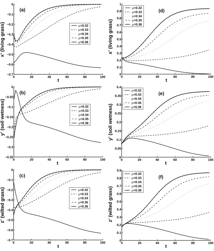
behaviour of CNOPs, we compute CNOPs under the same constraint condition δ=0.6 for GESs and δ=0.3 for DESs along the bifurcation diagram varying µ from 0.32 to 0.36 with step 0.01, and T =10.0 years. The components of the CNOPs of GESs and DESs are given in Table 3. The non-linear evolutions of the CNOPs are plotted in Fig. 5, which are obtained by calculating M( ¯U0µ+u
′∗
0µ)−M( ¯U0µ), where M is the nonlinear propagator of Eq. (1). ¯U0µis GES or DES
and u′0µ∗ is the CNOPs for the corresponding µ.
Figures 5a–c show that for moisture index µ=0.32, the CNOP with δ=0.6 induces a transition of the ecosystem from GES to DES. When µ increases, GES becomes more nonlin-early stable, and the evolutions of CNOPs with the same con-straint condition will not yield such transition. Figures 5d–f show that for µ=0.33, 0.34, 0.35 and 0.36, the CNOP with
δ=0.3 induce transitions of the ecosystem from DES to GES.
Figure 3 shows that for µ=0.32 and δ=0.3, there is no tran-sition of ecosystem. When the moisture index increase, DES becomes more nonlinearly unstable.
0 20 40 60 80 100 −0.7 −0.6 −0.5 −0.4 −0.3 −0.2 −0.1 0 t x’ (living grass) µ=0.32 µ=0.33 µ=0.34 µ=0.35 µ=0.36 (a) 0 20 40 60 80 100 0 0.1 0.2 0.3 0.4 0.5 0.6 0.7 0.8 0.9 1 t x’ (living grass) µ=0.32 µ=0.33 µ=0.34 µ=0.35 µ=0.36 (d) 0 20 40 60 80 100 −0.35 −0.3 −0.25 −0.2 −0.15 −0.1 −0.05 0 t
y’ (soil wetness)
µ=0.32 µ=0.33 µ=0.34 µ=0.35 µ=0.36 (b) 0 20 40 60 80 100 0 0.05 0.1 0.15 0.2 0.25 0.3 0.35 0.4
y’ (soil wetness)
t µ=0.32 µ=0.33 µ=0.34 µ=0.35 µ=0.36 (e) 0 20 40 60 80 100 −0.7 −0.6 −0.5 −0.4 −0.3 −0.2 −0.1 0 t z’ (wilted grass) µ=0.32 µ=0.33 µ=0.34 µ=0.35 µ=0.36 (c) 0 20 40 60 80 100 0 0.1 0.2 0.3 0.4 0.5 0.6 0.7 0.8 0.9 t z’ (wilted grass) µ=0.32 µ=0.33 µ=0.34 µ=0.35 µ=0.36 (f)
Fig. 5. The 100-year nonlinear evolutions of CNOPs, x′, y′and z′are perturbations. (a), (b) and (c) for GESs with δ=0.6; (d), (e), (f) for DESs with δ=0.3.
0 20 40 60 80 100 0 0.1 0.2 0.3 0.4 0.5 0.6 t x (living grass) δ=0.20 δ=0.40 δ=0.50 δ=0.60 GES A (a) 0 20 40 60 80 100 −0.1 0 0.1 0.2 0.3 0.4 0.5 0.6 t x (living grass) δ=0.20 δ=0.30 δ=0.50 DES B (d) 0 20 40 60 80 100 0.35 0.4 0.45 0.5 0.55 0.6 0.65 0.7 t y (soil wetness) δδ=0.20=0.40 δ=0.50 δ=0.60 GES A (b) 0 20 40 60 80 100 0.35 0.4 0.45 0.5 0.55 0.6 0.65 0.7 t y (soil wetness) δ=0.20 δ=0.30 δ=0.50 DES B (e) 0 20 40 60 80 100 0 0.1 0.2 0.3 0.4 0.5 0.6
t
z (wilted grass)
δ=0.20 δ=0.40 δ=0.50 δ=0.60 GES A(
c
)
0 20 40 60 80 100 −0.1 0 0.1 0.2 0.3 0.4 0.5 0.6t
z (wilted grass)
δ=0.20 δ=0.30 δ=0.50 DES B(
f
)
Fig. 6. The 100-year nonlinear evolution of the ecosystem, with LSVs plus equilibrium states as the initial conditions, left (right) column:
0 20 40 60 80 100 0 0.1 0.2 0.3 0.4 0.5 0.6
t
x (living grass)
CNOP LSV GES A(
a
)
0 20 40 60 80 100 −0.1 0 0.1 0.2 0.3 0.4 0.5 0.6 t x (living grass) CNOP LSV DES B (d) 0 20 40 60 80 100 0.35 0.4 0.45 0.5 0.55 0.6 0.65 0.7 0.75 t y (soil wetness) CNOP LSV GES A (b) 0 20 40 60 80 100 0.35 0.4 0.45 0.5 0.55 0.6 0.65 0.7 0.75 t y (soil wetness) CNOP LSV DES B (e) 0 20 40 60 80 100 0 0.1 0.2 0.3 0.4 0.5 0.6t
z (wilted grass)
CNOP LSV GES A(
c
)
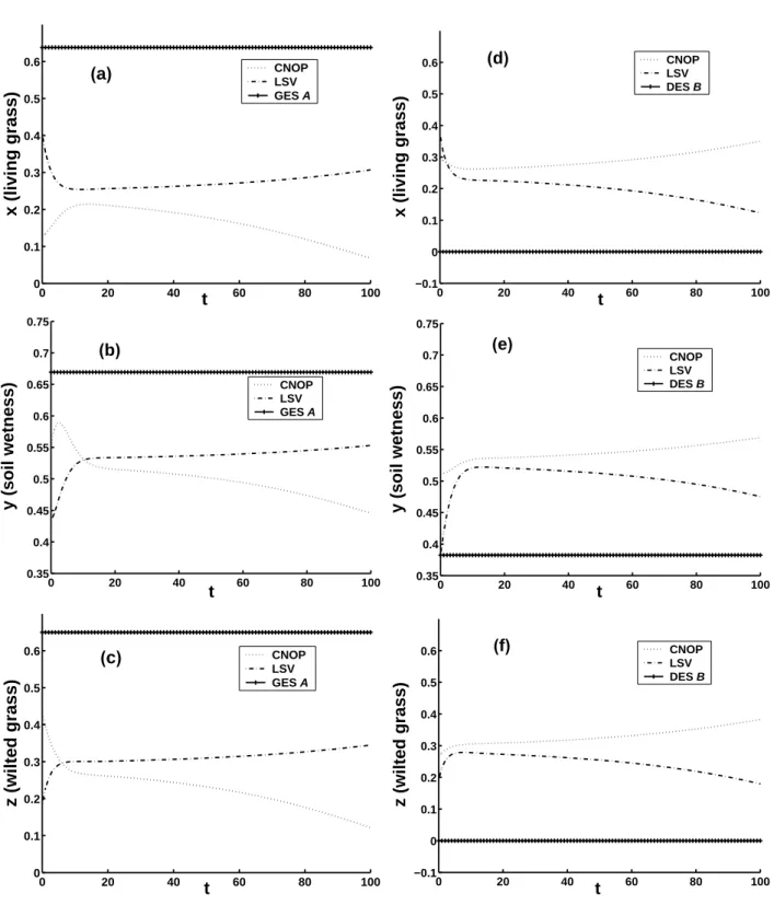
0 20 40 60 80 100 −0.1 0 0.1 0.2 0.3 0.4 0.5 0.6 t z (wilted grass) CNOP LSV DES B (f)Fig. 7. Nonlinear evolutions of the ecosystem, left (right) column: GES A (DES B) plus CNOPs and LSVs as the initial conditions with
0.310 0.32 0.33 0.34 0.35 0.36 0.37 0.38 0.2 0.4 0.6 0.8 1 1.2 1.4
µ
δ
cNonlinearly unstable
Nonlinearly stable
(
a
)
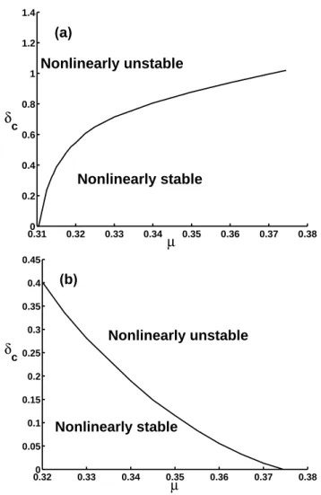
0.320 0.33 0.34 0.35 0.36 0.37 0.38 0.05 0.1 0.15 0.2 0.25 0.3 0.35 0.4 0.45 µ δ c Nonlinearly unstable Nonlinearly stable (b)Fig. 8. The critical value of δcvs. the parameter, moisture index, µ. (a) for GES; (b) for DES.
3.2 Comparison between the results obtained by ap-proaches of CNOPs and linear singular vectors To further explore the nonlinear feature of the ecosystem, linear singular vectors (LSVs) of GESs and DESs are cal-culated. Comparisons between their nonlinear evolutions are also made.
LSVs are obtained numerically by maximizing a modified version of objective function J in Eq. (4), which is obtained by replacing M in J by its tangent linear model. For GES
A and DES B with δ=0.2, T =10.0 years and moisture index µ=0.32, LSVs are (−0.082340, −0.082715, −0.162414) and
(0.177834, 0.000, 0.091516) respectively. For other δ, LSV can be obtained by multiplying them with a proper factor according to the linear characteristic. Comparing these LSVs with the CNOPs presented in the first row of Table 1, we observe distinct differences of the patterns in the phase space.
The differences between CNOPs and LSVs are not only represented by their patterns, but also by the behaviour of the evolutions of the ecosystem with GES and DES plus LSVs as initial conditions, which is obtained by calculating
M( ¯U0+u
′l
0δ), where M is the nonlinear propagator of Eq. (1).
u′0δl is the LSVs of the corresponding GES A or DES B. The left (right) column of Fig. 6 shows the components of GES A (DES B) and those of the nonlinear evolutions of the ecosys-tem with LSVs plus GES A (DES B) as initial conditions. It is clear from the left columns of Figs. 2, 3 and Fig. 6 that the evolutions of the ecosystem caused by CNOPs are larger than the corresponding ones by LSVs. Particularly, for δ=0.6, the CNOP induces a transition from the grassland to the desert much fast than the corresponding LSV.
Furthermore the differences of CNOPs and LSVs are demonstrated by the fact that in some cases, for the same magnitude, CNOPs yields a transition but LSVs does not. For example, for GES A with δ=0.57 and T =10.0 years, CNOPs (−0.564252, −0.080339, −0.152529) gives a tran-sition, but LSVs (−0.234616, −0.235632, −0.462961) does not, which is shown in the left column of Fig. 7. And for δ=0.42 and T =10.0, CNOPs (0.297454, 0.132069, 0.265479) also yield a transition, but LSVs (0.373516, 0.000, 0.192057) does not (see the right column of Fig. 7).
3.3 Sensitivity along the bifurcation diagram
It is clear from the subsection that in the bifurcation inter-val (µ1, µ2), although linear analysis shows that GES (DES)
is linearly stable, it can become nonlinearly unstable with a finite-amplitude initial perturbation, which means that a large enough initial perturbation will induce a transition from GES (DES) to DES (GES). The implication is, for each µ in
(µ1, µ2), a critical value, δc, the threshold for the magni-tude of initial perturbations must exist such that GES (DES) is nonlinearly stable when δ<δc, and vice versa. Now the question is how to find these thresholds. Mu et al. (2004) showed that the methodology of CNOPs provides a means for such a purpose. Following their work, we obtain the δc for µ in (µ1, µ2), and present the results in Fig. 8.
It follows from Fig. 8 that the threshold curve separates the plane into two parts. When the magnitude of CNOPs is larger than δc, the ecosystem evolves to DES (GES) with the CNOPs being initial perturbation, which implies that the ecosystem is nonlinearly unstable. If the magnitude of ini-tial perturbations is smaller than δc, the perturbations would drive the ecosystem recovering back to GES (DES). This also confirms the existence of the multiple-equilibrium state for the grassland ecosystem from another point of view. When
µ decreases (increases), GES (DES) become more and more
Table A1. Values of parameters and coefficients.
Dimensional parameters Dimensionless coefficients
x∗ 0.1 Kg m−2 β, βz, γ 0.1 y∗ 240 mm γ 0 z∗ 0.1 Kg m−2 αz 0.5 α∗ 0.4 Kg m−2yr−1 σf, εg, εg′, εd, εd′, εc 1.0 e∗ 1000 mm yr−1 εdz, εcz 1.0 – – φrs 0.7 – – λ 0.015 – – κ1 0.3 – – κ1′′ 0.4 – – κ1′ 1.0 – – ε1, ε1′′ 0.7 – – ε1, ε2, ε′2, ε ′′ 2, ε3, ε ′′ 3 1.0
4 Summary and discussion
Within a simple theoretical model, we have addressed the nonlinear stability and sensitivity of the grassland ecosystem to finite-amplitude initial perturbations.
The results obtained show that the moisture index µ plays an essential role in this grassland ecosystem. When µ is less than the bifurcation point µ1, DES is nonlinearly stable, no
matter how large the initial finite-amplitude perturbation is. This implies that human activities and natural factors of in-stantaneous or short type can not change the natural desert state. In case of µ being larger than the bifurcation point µ2,
GES is conditionally nonlinearly stable, which means that if
δ< ¯x, no initial perturbations including CNOPs would yield
a transition from it to DES, but for δ≥ ¯x, if we make a
de-structive action, such that the initial value of x is null, the ecosystem will evolve to DES. This suggests that, even if the soil is washy and the natural condition is feasible, it is still important to keep the balance for the ecosystem. When
µ is between µ1and µ2, the grassland ecosystem is fragile,
GES (DES) is linearly stable but nonlinearly unstable, which means that a large enough initial finite-amplitude perturba-tion can induce a transiperturba-tion from GES (DES) to DES (GES). This suggests the importance of the management of human activities when moisture index µ is in (µ1, µ2).
The approach of CNOPs also allows us to determine the threshold, the critical value δc, which is the smallest magni-tude of the finite-amplimagni-tude perturbation that induces a tran-sition from GES (DES) to DES (GES). For GES (DES), the critical value δc decreases to zero as µ approaches the bi-furcation point µ1(µ2). This explains how the steady states
lose their stability when the bifurcation point µ1(µ2) is
ap-proached.
The negativeness (positiveness) of the z-component of CNOPs for GES (DES) shown in Tables 1–3 demonstrates that the shading effect of wilted grass is very important for the maintenance of GES and for the improvement of DES.
That is, thinking about a general effect of all factors and adopting comprehensive actions, such as planting grass, ir-rigating measurable and shading the ground with dead leaves etc. at the same time can improve the ecosystem. This ac-cords with the viewpoint of Zeng et al. (2004, 2005a, b).
The results also show that CNOPs is a useful tool in the investigation of the characteristics of nonlinear ecosystems. This method is currently being generalized to be applicable to much more complex models with more degrees of free-dom. The aim is to tackle these problems eventually in the course of drought in North China by considering the human activities and natural factors. It is expected that the approach may provide quantitative bounds on perturbations of the land ecosystem, and yields more insights into the land ecosystem. Whether the results obtained in this paper depend on the norm is an interesting problem. Besides, it is also worthwhile to use other approaches, such as the bred vector of Toth and Kalnay (1997), the Lyapunov vector and its nonlinear exten-sion recently proposed by Ding and Li (2006), etc., to deal with the stability and sensitivity problems of ecosystems. We leave all these to future studies.
Appendix A
A brief introduction of the three-variable ecosys-tem model
This appendix will introduce the three-variable ecosystem model developed by Zeng et al. (2004). The model is com-posed of three ordinary differential equations, in Eqs. (1a) and (1c)
G = α∗(1 − e−εgx)(1 − e−ε′gy)
D = α∗β(eεdx− 1)(1 − e−ε′dy)−1
Gz= α∗αzβ(eεdx− 1)(1 − e−ε ′ dy)−1 Dz= α∗βz(eεdzz− 1) and Cz= α∗γz(1 − eεczz)
where dimensional parameter α∗ is the maximum growth rate, the dimensionless coefficients β, γ , βz, and γzare ratios of the maximum or characteristic rates of the corresponding process over α∗, αzis the rate of wilted grass accumulation, and ε’s with different subscripts are exponential attenuation coefficients (Zeng et al., 2004, 2005b).
The Eq. (1b) is based on the vegetation-soil interaction. The evaporation term are
Es=e∗(1−e−ε2y)e−ε3z((1−σf)+σf(1−κ1(1−e−ε1x)))
where e∗is the potential evaporation, κ1is the correction due
to the non-opaque cover of the living grass for the diffusive radiation, and the fraction of living grass coverage, σf, is described by σf=1−e−εfx, where εf is a coefficient, and differ from εgx, depending on the shape and distribution of leaves. Transpiration term Er = e∗φrs(1 − e−ε ′ 2y)σf(1 − κ′ 1e −ε′1x)
where φrsis the ratio of potential transpiration to e∗, and κ1′ is coefficient. The moisture index µ=P /e∗ substituted the precipitation term P . Finally, the runoff is
R = λe∗µ(eε ′′ 2y− 1)eε ′′ 3z((1 − σf) + σf(1 − κ′′ 1(1 − e ε1′′x)))
where λ and κ1′′are coefficients.
All parameters and coefficients are given in Zeng et al. (Ta-ble 1, 2004). Here, we give their values again for the sake of convenience (Table A1).
Acknowledgements. The authors thank the reviewers for their valuable suggestions. M. Mu and B. Wang are supported by the state Key Development Program for Basic Research (Grant
No. 2006CB400503), the KZCX3-SW-230 of the Chinese
Academy of Sciences (CAS) and National Natural Science Foun-dation of China (No. 40675030). In addition B. Wang is supported by K. C. Wang Education Foundation, Hong Kong and the National Postdoctoral Science Foundation of China.
Edited by: U. Feudel
Reviewed by: three anonymous referees
References
Birgin, E. G., Mart´ınez, J. M., and Raydan, M.: Nonmonotone spec-tral projected gradient methods on convex sets, SIAM Journal on Optimization, 10, 1196–1211, 2000.
Birgin, E. G., Mart´ınez, J. M., and Raydan, M.: Algorithm 813: SPG–software for convex–constrained optimization, ACM Transactions on Mathematical Software, 27, 340–349, 2001. Birgin, E. G., Mart´ınez J. M., and Raydan, M.: Inexact Spectral
Projected Gradient Methods on Convex Sets, IMA Journal of Numerical Analysis, 23, 539–559, 2003.
Brovkin, V., Claussen, M., Petoukhov, V., and Ganopolski, A.: On the stability of the atmosphere–vegetation system in the Sa-hara/Sahel region, J. Geophys. Res. 103, 31 613–31 624, 1998. Claussen, M., Kubatzki, C., Brovkin, V., Ganopolski, A.,
Hoelz-mann, P., and Pachur, H.: Simulation of an abrupt change in Sa-haran vegetation in the mid-Holocence, Geophys. Res. Lett., 26, 2037–2040, 1999.
Ding, R. and Li, J.: Nonlinear finite-time Lyapunov exponent and predictability, Phys. Lett. A, 364, 396–400, 2007.
Duan, W. S., Mu, M., and Wang, B.: Conditional nonlinear optimal perturbations as the optimal precursors for El Nino– Southern Oscillation events, J. Geophys. Res., 109, D23105, doi:10.1029/2004JD004756, 2004.
Duan, W. S. and Mu, M.: Investigating decadal variability of El Nino–Southern Oscillation asymmetry by conditional non-linear optimal perturbation, J. Geophys. Res., 111, C07015, doi:10.1029/2005JC003458, 2006.
Klausmeier, C. A.: Regular and irregular patterns in semiarid vege-tation, Science, 284, 1826–1828, 1999.
Mu, M., Duan, W. S., and Wang, B.: Conditional nonlinear optimal perturbation and its applications, Nonlin. Processes Geophys., 10, 493–501, 2003a.
Mu, M., Duan, W. S., and Wang, B.: Season-dependent dynamics of nonlinear optimal error growth and El Nino–Southern Oscilla-tion predictability in a theoretical model, J. Geophys. Res., 112, D10113, doi:10.1029/2005JD006981, 2007a.
Mu, M. and Duan, W. S.: A new approach to studying ENSO pre-dictability: conditional nonlinear optimal perturbation, Chinese Sci. Bull., 48, 1045–1047, 2003b.
Mu, M., Sun, L., and Dijkstra, H. A.: The sensitivity and stability of the ocean’s thermohaline circulation to finite amplitude per-turbations, J. Phys. Ocean., 34, 2305–2315, 2004.
Mu, M., Xu, H., and Duan, W. S.: A kind of initial errors related to “spring predictability barrier” for El Nino events in Zebiak–Cane model, Geophys. Res. Lett., 34, L03709, doi:10.1029/2006GL027412, 2007b.
Sun, L., Mu, M., Sun, D. J., and Yin, X. Y.: Passive mechanism of decadal variation of thermohaline circulation, J. Geophys. Res., 110, C07025, doi:10.1029/2005JC002897, 2005.
Toth, Z. and Kalnay, E.: Ensemble forecasting at NCEP and the breeding method, Mon. Wea. Rev., 125, 3297–3319, 1997. UNEP(United Nations Environmen Programme): World Atlas of
Desertification, Edward Arnold, London, 1992.
Zeng, N. and Neelin, J. D.: The role of vegetation-climate interac-tion and interannual variability in shaping the African savanna, J. Climate, 13, 2665–2670, 2000.
Zeng, N., Hales, K., and Neelin, J. D.: Nonlinear Dynamics in a Coupled Vegetation-Atmosphere System and Implications for Desert-Forest Gradient, J. Climate, 15, 3474–3487, 2002. Zeng, Q. C., Lu, P. S., and Zeng, X. D.: Maximum simplified
dy-namic model of grass field ecosystem with two variables, Sci. China Ser. B, 37, 94–103, 1994.
field ecosystem with two varibles, Ecol. Model., 85, 187–196, 1996.
Zeng, X. D., Shen, S. S. P., Zeng, X. B., and Dickinson, R. E.: Mul-tiple equilibrium states and the abrupt transitions in a dynamical system of soil water interacting with vegetation, Geophys. Res. Lett., 31, 5501, doi:10.1029/2003GL018910, 2004.
Zeng, X. D., Wang, A. H., Zhao, G., Shen, S. S. P., Zeng, X. B., and Zeng, Q. C.: Ecological dynamic model of grassland and its practical verification, Sci. China Ser. C, 48, 41–48, 2005a. Zeng, X. D., Zeng, X. B., Shen, S. S. P., Dickinson, R. E., and
Zeng, Q. C.: Vegetation–soil water interaction within a dynami-cal ecosystem model of grassland in semi-arid areas, Tellus, 57B, 189–202, 2005b.