HAL Id: hal-00296433
https://hal.archives-ouvertes.fr/hal-00296433
Submitted on 7 Feb 2008
HAL is a multi-disciplinary open access
archive for the deposit and dissemination of
sci-entific research documents, whether they are
pub-lished or not. The documents may come from
teaching and research institutions in France or
abroad, or from public or private research centers.
L’archive ouverte pluridisciplinaire HAL, est
destinée au dépôt et à la diffusion de documents
scientifiques de niveau recherche, publiés ou non,
émanant des établissements d’enseignement et de
recherche français ou étrangers, des laboratoires
publics ou privés.
Eddy covariance measurements of sea spray particles
over the Atlantic Ocean
S. J. Norris, I. M. Brooks, G. de Leeuw, M. H. Smith, M. Moerman, J. J. N.
Lingard
To cite this version:
S. J. Norris, I. M. Brooks, G. de Leeuw, M. H. Smith, M. Moerman, et al.. Eddy covariance
measure-ments of sea spray particles over the Atlantic Ocean. Atmospheric Chemistry and Physics, European
Geosciences Union, 2008, 8 (3), pp.555-563. �hal-00296433�
www.atmos-chem-phys.net/8/555/2008/ © Author(s) 2008. This work is licensed under a Creative Commons License.
Chemistry
and Physics
Eddy covariance measurements of sea spray particles over the
Atlantic Ocean
S. J. Norris1, I. M. Brooks1, G. de Leeuw1,2, M. H. Smith1, M. Moerman3, and J. J. N. Lingard1
1School of Earth and Environment, University of Leeds, Leeds, LS2 9JT, UK
2University of Helsinki, Dept. of Physical Sciences, Helsinki, Finland & Finnish Meteorological Institute, Climate and Global
Change Unit, Helsinki, Finland
3TNO, Defence and Security, The Hague, The Netherlands
Received: 17 August 2007 – Published in Atmos. Chem. Phys. Discuss.: 11 September 2007 Revised: 13 November 2007 – Accepted: 8 January 2008 – Published: 7 February 2008
Abstract. Most estimates of sea spray aerosol source func-tions have used indirect means to infer the rate of produc-tion as a funcproduc-tion of wind speed. Only recently has the tech-nology become available to make high frequency measure-ments of aerosol spectra suitable for direct eddy correlation determination of the sea spray particle flux. This was ac-complished in this study by combining a newly developed fast aerosol particle counter with an ultrasonic anemometer which allowed for eddy covariance measurements of
size-segregated particle fluxes. The aerosol instrument is the
Compact Lightweight Aerosol Spectrometer Probe (CLASP) – capable of measuring 8-channel size spectra for mean radii between 0.15 and 3.5 µm at 10 Hz. The first successful mea-surements were made during the Waves, Air Sea Fluxes, Aerosol and Bubbles (WASFAB) field campaign in October 2005 in Duck (NC, USA). The method and initial results are presented and comparisons are made with recent sea spray source functions from the literature.
1 Introduction
Sea spray particles are salt water droplets ejected from the ocean. The aerosols formed from sea spray particles are im-portant because they have a significant impact on climate processes, both directly via the scattering of solar radia-tion, and indirectly via their influence on cloud microphysi-cal properties. Sea salt particles are the single most important factor controlling the scattering of solar radiation and, hence, the radiation budget near the surface under cloud free condi-tions over the open oceans (Haywood et al., 1999). They dominate the particulate mass concentration in unpolluted marine air and contribute approximately 44% to the global Correspondence to: S. J. Norris
(s.norris@see.leeds.ac.uk)
aerosol mass flux into the atmosphere (Seinfeld and Pandis, 1998). They act as cloud condensation nuclei and have a large influence on both the microphysics and chemistry of marine stratocumulus clouds (O’Dowd et al., 1999), which are one of the largest sources of uncertainty in climate pre-dictions. They have a large range of sizes, with dry radii from 0.01 µm up to 100 µm (M˚artensson et al., 2003; Clarke et al., 2006).
Sea spray aerosol droplets are produced by several differ-ent mechanisms. Jet and film droplets are produced from bursting bubbles. Bubbles form predominantly from break-ing waves, but there are many other possible production mechanisms: biological processes, de-gassing of air-rich sur-face layers as water is warmed, volcanic release of gases, and rain impacting on the ocean surface. For 10-m wind speeds
above about 5 m s−1 the wind stress at the ocean surface
is sufficient to cause breaking waves (Lewis and Schwartz, 2004). As they break, the waves entrain air into the water producing a plume of bubbles (Blanchard and Woodcock, 1980). As the bubbles reach the ocean surface, patches of white foam form – whitecaps. As a bubble protrudes above the ocean surface some of the liquid film surrounding the bubble drains off, thinning and weakening the film. The film ruptures and rolls back on itself before producing film droplets (Blanchard and Woodcock, 1980; Spiel, 1998). Jet droplets are produced when the pressure is released from
inside the bubble as it collapses. A liquid jet shoots up
from the base of the bubble cavity due to hydrostatic forces, quickly becomes unstable and breaks into a small number of jet droplets (Blanchard, 1983).
The sea spray source function (SSSF) describes the amount (number, volume, mass) of sea spray aerosol pro-duced at the sea surface per unit time and area as a func-tion of environmental condifunc-tions. SSSF’s available in the literature vary by as much as 6 orders of magnitude (An-dreas, 1998, 2002); however, results from recent work in the
556 S. J. Norris et al.: EC fluxes of sea spray sub-micron size-range converge to within about a factor of
about 7 (Clarke et al., 2006). Most of the source functions are derived from indirect methods, relying either on an as-sumption of steady state in the atmosphere or the whitecap method. In the former the production flux is assumed equal to a known deposition flux (e.g., Andreas, 1992; Smith et al., 1993; Fairall et al., 1994; Smith and Harrison, 1998); in the latter a parameterization of the fractional whitecap cover, based on field observations, is combined with lab-oratory measurements of the sea spray aerosol production rate per unit area of whitecap (e.g. Monahan et al., 1986; M˚artensson et al., 2003). For recent formulations of the sea spray source function, see Schulz et al. (2004) and O’Dowd and de Leeuw (2007).
There are potential problems associated with the assump-tion of steady state leading to balance between producassump-tion and removal of sea spray particles (e.g., Fairall et al., 1994; Smith et al., 1993; Smith and Harrison, 1998). A direct mea-surement of the aerosol flux would eliminate some, though not all, of these problems, and would be expected to re-sult in a physically more robust source function. The ideal approach to turbulent flux measurement is eddy covariance. This method has been used to measure particle deposition to forests (Gallagher et al., 1997; Buzorius et al., 1998) and re-cently also to look at the production flux of sea salt particles (Nilsson et al., 2001; Geever et al., 2005). The eddy covari-ance method correlates turbulent fluctuations of the vertical wind component with those of particle concentration. The vertical wind speed is usually measured with an ultrasonic anemometer. The vertical turbulent flux is obtained from the equation for total vertical flux via Reynolds averaging (see Stull, 1988). Application of the EC method requires an in-strument that can measure aerosol concentrations with a high temporal resolution – eddy correlation requires a minimum instrument response of 2–3 Hz – combined with a high sple volume in order to achieve robust statistics with low am-bient particle concentrations. The measurements of sea spray fluxes that have been made to date have either not been size segregated or had a low temporal resolution. The number of measurements also remains sparse due to the bulky and ex-pensive nature of most of the aerosol instrumentation, which makes it awkward to use close to the sea surface without ei-ther causing flow distortion or risking damage to the instru-mentation in a hostile environment.
The eddy covariance method was first applied to the mea-surement of sea spray fluxes by Nilsson et al. (2001), who assembled a flux package consisting of a sonic anemome-ter and a Condensation Particle Counanemome-ter (CPC). The CPC used had a temporal resolution of 3 Hz and measured the to-tal particle concentration for radii larger than 10 nm. Geever et al. (2005) used a flux package consisting of a sonic anemometer and two CPC’s to determine fluxes in two very broad size ranges. de Leeuw et al. (2007) have recently made eddy covariance flux estimates in four coarse and overlap-ping size ranges using a Passive Cavity Aerosol
Spectrome-ter Probe (PCASP). The PCASP time resolution is only 1 Hz, however, so not all the turbulent fluctuations can be resolved. The objective of this paper is to demonstrate the feasibility of making fully size-resolved sea spray flux measurements via eddy covariance using a novel aerosol instrument devel-oped at the University of Leeds that couples a high sample volume to fast time response. The Compact Light-weight Aerosol Spectrometer Probe (CLASP) version used here can measure particles with ambient radii in the range 0.15 µm to
3.5 µm. It has a flow rate of 50 ml s−1and a sample rate of
10 Hz. The main component of CLASP is a MetOne Optical Particle Counter (OPC) from Pacific Scientific Instruments. Particles in the MetOne sample volume scatter light from a laser (wavelength 780 nm). The light scattered in the side lobes is detected by a photodiode; its intensity is a measure of the particle’s size. In CLASP the MetOne OPC is con-nected to an 8 channel pulse height analyser to classify the peaks in output signal into 7 bins. See Hill et al. (2007) for more technical details of CLASP.
The CLASP instrument is especially suitable for in-situ flux measurements in combination with an ultra-sonic anemometer because of its small size (approximately 11×15×6 cm) and light weight, which allows co-location with the sonic anemometer without causing significant flow distortion, and thus minimizing the length of inlet tube re-quired (here approximately 0.5 m) and hence particle losses. A high flow rate ensures that adequate statistics can be achieved to characterize spectra within a time period of ap-proximately 10 min, similar to the typical averaging time re-quired for surface layer flux measurements.
2 Field campaign
The Waves, Air-Sea Fluxes, Aerosol and Bubbles (WAS-FAB) experiment (de Leeuw et al., 2007; Zappa et al., 2006) took place during October 2005 at the Army Corps of En-gineers Field Research Facility (FRF) in Duck, North Car-olina. The aim of the overall project was to obtain a large set of measurements to help constrain the sea spray source func-tion. The location in North Carolina was selected because of the 560 m long pier and supporting oceanographic and me-teorological observations available at the site. The measure-ment site was located at the end of the pier, well beyond the surf zone. Initial micrometeorological measurements made at the same location during the winter of 2005/2006 demon-strated that the local drag coefficient compared favourably with that obtained from the TOGA-COARE bulk flux param-eterization (Zappa et al., 2006); we thus have confidence that the site is reasonably representative of the open ocean under
onshore wind conditions (directions from 5◦to 120◦).
The flux package used here (Fig. 1) consisted of a Gill R3A ultrasonic anemometer and CLASP, and was situated on a lattice tower at 16.5 m above the mean sea surface at the end of the pier. The measurements were supported by a second
Fig. 1. Flux system consisting of the ultrasonic anemometer and
the CLASP sensor (black cube) mounted at the end of a metal arm. The CLASP inlet tube can be kept short, roughly 0.5 m, because the sensor of CLASP is very small and thus does not perturb the air flow to the ultrasonic anemometer.
aerosol flux package consisting of an ultrasonic
anemome-ter, CPC and OPC with a heated inlet at 300◦C and a Licor
LI-7500 open path H2O/CO2gas analyzer. Supporting
in-struments included a sea spray package consisting of three Particle Metric Systems instruments: the Forward Scatter-ing Spectrometer, the Optical Aerosol Probe, and a PCASP to provided background aerosol spectra. Information on the mass of carboniferous aerosol in the air sample was pro-vided by a Magee Scientific Aethalometer. Meteorological stations provided information on the local temperature, hu-midity, wind speed and direction; offshore buoys provided wave measurements.
Flux losses due to displacement between the sonic anemometer and the CLASP inlet were calculated using the method described in Kristensen et al. (1997) to be 0.2%. The time delay between a particle entering the CLASP inlet tube and entering the MetOne sample volume was calculated to be 0.2 s; this is in good agreement with the 2-sample offset obtained by determining the time lag required to maximize the covariance between the turbulent vertical velocity and the CLASP concentrations. This offset was applied to the CLASP time series prior to calculating the turbulent fluxes.
3 Data processing
It is important to ensure that the averaging time for flux cal-culations is sufficient for all eddy scales contributing to the turbulent flux of particles to be sampled by the flux pack-age, but not so long that non-turbulent mesoscale variability
10−4 10−3 10−2 10−1 100 101 −0.05 0 0.05 0.1 0.15 dN/dR µ m −1 m −2 s −1 Frequency HZ 10−4 10−3 10−2 10−1 100 101 −0.2 −0.15 −0.1 −0.05 0 <w’u’> ms −1 15:00 − 15:20 15:20 − 15:40 15:40 − 16:00 0.15 µm 0.16 µm 0.19 µm 0.24 µm 0.59 µm 1.25 µm 2.25 µm
Fig. 2. Ogive curves for the momentum flux (top) and aerosol flux
(bottom) for the sizes indicated in the legend. Each curve in the lower panel is the average of the three consecutive 20 min periods from 12 October shown in the upper panel.
is included. Very low frequency perturbations can be caused by non-stationarity of the local flow. Non-stationarity can occur during frontal passages, rapid boundary layer growth or decay, or other short-term boundary layer disturbances such as the passage of clouds. They can be identified as periods when the time series varies in a systematic, non-turbulent, way (Massman and Lee, 2002). An averaging time of about 30 min is generally considered a reasonable compro-mise (Massman and Lee, 2002). An appropriate averaging time for a given data set can be determined from the cumu-lative integral, from high frequency to low, of the cospec-trum – the so-called Ogive function. Friehe et al. (1988) and Desjardins et al. (1989) used this method to find the mini-mum frequency contributed by turbulent eddies, and hence the minimum averaging time required to include all flux con-tributions. The frequency at which the slope of the Ogive curve levels off indicates the maximum scale of contributing eddies. Figure 2 shows example Ogive curves for the mo-mentum and aerosol fluxes. The momo-mentum flux is a good indicator of the scale of turbulent eddies; this levels off at around 0.003 Hz (approximately 5.5 min). An averaging pe-riod of 20 min should thus encompass all contributing eddies, averaging several of the largest scale, and is used though-out this investigation. Some low-frequency variability remains visible in the ogives for aerosol flux. This is interpreted as being due to non-stationarity, or mesoscale variability, in the aerosol concentrations.
3.1 Effects of aerosols other than sea spray
In order to reliably estimate the flux of sea spray aerosol, it must be ascertained that the particles measured are indeed produced at the sea surface without significant contamination by non-sea spray particles. We thus require that the wind was onshore and the air mass sampled had resided over the ocean for between 3 and 4 days. During WASFAB, such conditions occurred only between 10 and 13 October 2005. Figure 3
558 S. J. Norris et al.: EC fluxes of sea spray −90 −85 −80 −75 −70 −65 −60 −55 −50 20 25 30 35 40 45 Longitude Latitude coastline 10th October 2005 11th October 2005 12th October 2005
Fig. 3. Back trajectories from the NOAA Hysplit model for the 10
to 12 October 2005.
shows an example back trajectory from the NOAA Ready Hysplit model for 11 October.
Clean maritime air masses might still include non-sea-salt particles from di-methylsulphide (DMS) derived new particle formation or dust particles from the Saharan desert via long range transport. DMS-derived sulphate particle production is at its highest in the summer when stratification of the wa-ter column is greatest and the mixing depths are shallowest (Kiene, 1999), and occurs primarily over plankton blooms. DMS production can occur in October on the east US coast; however, there were no plankton blooms in the area during the field campaign and chlorophyll concentrations mapped
by the NASA Terra satellite were below 1 mg m−3. Thus, we
conclude there was limited biological activity to sustain local DMS production.
Any dust measured during this project would most likely originate in the Sahara and be transported into the atmo-sphere under high wind speed conditions. An examination of NASA Ozone Monitoring Instrument aerosol index im-ages for the week preceding the October 11 indicates that there were no significant dust events in northern Africa. The aerosol index was consistently low for the northern part of Africa for the whole of September and October. Further-more, air mass trajectories show that the air masses sam-pled had been over the ocean for at least 5 days and had turned back from the Northern American continent to a west-erly course over the ocean before reaching the site in Duck. Hence it is very unlikely that dust would appear in these air masses in quantities significant enough to influence the mea-surements. 60 80 100 RH (%) 15 20 25
water air temp ( oC) 0 5 10 15 wind speed (m/s) 0 200 wind direction 5 10 wave period (s) 0 50 100 wave direction 1 1.5 2 wave height (m) 12.00 18:00 11th 06.00 12.00 18.00 12th 06.00 12.00 18.00 00.00 −1 −0.5 0 0.5 stability
Date and Time
Fig. 4. Summary of the local meteorological and oceanic conditions
over the onshore wind period between the 10 and the 12 October 2005 at the FRF pier in Duck, N.C. The dashed curve on the wa-ter and air temperature graph in the air temperature while the solid curve is the water temperature.
Any non-sea-salt aerosols originating elsewhere would only contribute to the deposition flux. The net flux measured with the eddy covariance method is the sum of the upward flux of particles locally produced at the sea surface and the downward flux of particles produced elsewhere and advected into the measurement region.
4 Results
4.1 Summary of local meteorological and oceanic
condi-tions
Synoptic conditions between 10 and 12 October 2005 were dominated by a weak low pressure system that tracked just offshore of the east coast of the United States, moving from
south to north. As it moved north the system deepened
slightly and the wind speed increased from 3 to 12 m s−1over
the three days. Figure 4 shows a summary of the local meteo-rological and oceanic conditions during this time period. The
wind direction remained consistently between 5◦and 120◦,
apart from a few short occasions, in particular during a short
102 104 106 108 102 104 106 108 102 104 106 108 dF/dr µ m −1 m −2 s −1 102 104 106 108 4 6 8 10 12 102 104 106 108 windspeed ms−1 4 6 8 10 12 102 104 106 108 windspeeds ms−1 a) b) c) d) e) f) r2 = 0.77 r2 = 0.65 r2 = 0.67 r2 = 0.67 r2 = 0.81 r2 = 0.62 0.15 µm 0.16 µm 0.19 µm 0.24 µm 0.59 µm 1.25 µm
Fig. 5. Flux versus mean wind speed for mean particle radius (a)
0.15 µm, (b) 0.16 µm, (c) 0.19 µm, (d) 0.24 µm, (e) 0.5 µm, (f) 1.2 µm. Solid lines are log-linear fits to the data, dotted lines show the 95% confidence limits of the fit.
period from 15:00 till 19:00 UTC on the 10 October; data from these periods were excluded from the analysis. The mean half-hour averaged wave heights increased from ap-proximately 1 to 2 m over the 3 days; the mean wave period remained almost constant at approximately 10 s up to 20:00 on 11 October, then decreased rapidly to approximately 5 s by 00:00 on 12 October; these changes, and an associated shift in the dominant wave direction were driven by the pas-sage of the low pressure north offshore of the measurement site. Wave periods then increased slowly to 9 s by the end of 12 October, with a few short intervals of longer periods, cor-responding with changes in wave direction. Both the air and water temperatures decreased over the measurement period; air temperature at a greater rate than the water temperature. The air-sea temperature difference is negative, providing a convective atmospheric surface layer, for all but one occa-sion over the period of 10 to 12 October. A positive air-sea temperature difference occurred at 01:00 on 11 October, and results from a drop in the water temperature which lasted for about 2 h; this resulted in a short period of stable condi-tions in the atmospheric surface layer. For the majority of the measurement period the atmosphere was either unstable or near-neutral.
4.2 Size segregated fluxes
The data were first screened for wind sector. Only periods when the instruments were all working and the local wind
di-rection was consistently between 5◦and 120◦were accepted,
producing a total of 20 20-min averaged flux estimates, under
a range of wind speeds from 4 to 12 ms−1.
10−2 10−1 100 101 102 10−2 100 102 104 106 108
Sea spray source functions for wind speed 5 m/s
radius r80 [µm] dF/dr 8 0 [ µ m −1 s −1 m −2 ] Monahan 86 M86−extrapol Andreas 98 Martensson 03 Reid et al. 01 de Leeuw et al. 03 Clarke 06 This work (a) 10−2 10−1 100 101 102 10−2 100 102 104 106 108
Sea spray source functions for wind speed 10 m/s
radius r80 [µm] dF/dr 8 0 [ µ m −1 s −1 m −2 ] Monahan 86 M86−extrapol Andreas 98 Martensson 03 Reid 01 de Leeuw 03 Clarke 06 this work (b) 10−2 10−1 100 101 102 10−2 100 102 104 106 108
Sea spray source functions for wind speed 12 m/s
radius r80 [µm] dF/dr 8 0 [ µ m −1 s −1 m −2 ] Monahan 86 M86−extrapol Andreas 98 Martensson 03 Reid 01 de Leeuw 03 Clarke this work (c)
Fig. 6. Comparison of results from this work with a few sea spray
source functions available in the literature for a number of different wind speeds (a) 5 m−1, (b) 10 m s−1, (c) 12 m s−1.
Figure 5 presents the particle fluxes as a function of the mean horizontal wind speed at the 10-m level, for 6 of the 7 particle size bins. The 7th size bin is not shown because the Poisson statistics associated with low particle numbers at this largest size (aggravated by losses down the inlet tube) resulted in substantial signal noise. Log-linear fits to the data
560 S. J. Norris et al.: EC fluxes of sea spray
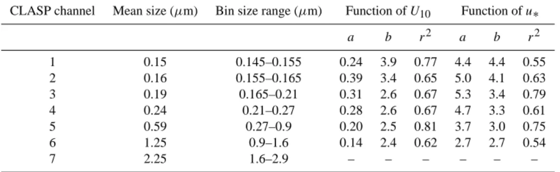
Table 1. Log-Linear fit parameters for each of the different particle sizes as functions of wind speed, U10, and friction velocity, u∗.
CLASP channel Mean size (µm) Bin size range (µm) Function of U10 Function of u∗
a b r2 a b r2 1 0.15 0.145–0.155 0.24 3.9 0.77 4.4 4.4 0.55 2 0.16 0.155–0.165 0.39 3.4 0.65 5.0 4.1 0.63 3 0.19 0.165–0.21 0.31 2.6 0.67 5.3 3.4 0.79 4 0.24 0.21–0.27 0.28 2.6 0.67 4.7 3.3 0.61 5 0.59 0.27–0.9 0.20 2.5 0.81 3.7 3.0 0.75 6 1.25 0.9–1.6 0.14 2.4 0.62 2.7 2.7 0.54 7 2.25 1.6–2.9 – – – – – –
show the strength of the relationship – nearly all the data points in each size range fall within the 95% confidence lim-its. For particles around 0.5 µm radius (Fig. 5e) a
correla-tion coefficient of r2=0.81 was found for a log-linear
rela-tionship. All other size ranges have correlation coefficients greater than 0.62. The log-linear relationship between the particle fluxes and wind speed has the form
log(dF /dr) = aU10+b (1)
where dF /dr is the flux for each particle size bin, U10 is
the mean horizontal wind speed at 10 m, and a and b are variables related to the particle size. Table 1 shows the values for a and b for each size range.
Sea spray fluxes are also often parameterized in terms of
friction velocity, u∗instead of U10. An advantage of using
u∗ is that in principle it takes account of some of the other
factors that may affect the flux, such as thermal stability and wave state (Geever et al., 2005). Relationships between the fluxes for various particle sizes and the measured friction ve-locity have been calculated and are also summarised in Ta-ble 1.
4.3 Comparison with sea spray source functions in the
lit-erature
The scope of this paper is to show that using the CLASP in-strument along with a sonic anemometer, the net fluxes of sea spray particles can be measured across a number of well-resolved size bins. There is the potential to calculate a sea spray source function with this method but due to the limited amount of data collected during the WASFAB campaign this is not possible here. A strict comparison of the net fluxes measured during WASFAB with SSSFs from the literature requires that a correction for the deposition velocity of parti-cles be applied. There is significant uncertainty in the deposi-tion velocities proposed in the literature for the size of
parti-cles measured here, ranging from 0.02% at 10 m s−1(Hopple
et al., 2005) up to 30% (Slinn and Slinn, 2001). Given this high degree of uncertainty we have not attempted to correct for deposition here and simply present the measured net flux.
Figure 6 shows a comparison of the measured net fluxes
with several SSSFs for wind speeds of 5 m s−1, 10 m s−1and
12 m s−1. All the source functions from the literature are
ap-plied for 80% relative humidity and denoted dF /dr80, (i.e.
particle radii are adjusted for to that which would be obtained under equilibrium conditions at a relative humidity of 80%). The measured net fluxes have also been adjusted to a 80% relative humidity using Gerber’s (1985) growth model.
Errors in direct covariance measurements are most likely due primarily to finite time averaging and to flow distortion effects (Frederickson et al., 1997). Two types of error analy-sis were conducted here. The first was to assess the system-atic errors induced by the instruments using the compound error method outlined by Blanc (1986). This method works on the principle of examining the differences between the computed variables assuming no errors and the computed variables assuming both positive and negative errors in each input variable. These measurement errors are associated with problems in the physical measurement of a parameter due to factors such as sensor accuracy, calibration errors, flow distortion (Frederickson et al., 1997), humidity fluctuations (Gallagher et al., 1997), and particle losses down the inlet tube (Davis, 1968). To calculate the systematic error associ-ated with fluxes of particles both the error in the measured vertical wind speed and the particle concentrations need to be determined.
The error in the vertical wind speed measured by the sonic anemometer, is quoted in the manual as 1.5% for wind speeds
between 0 and 60 m s−1; this value has been used previously
by Yelland et al. (1994). The error in the measured parti-cle number concentrations for each channel of CLASP was calculated by comparing the CLASP spectra to that of the PCASP. The CLASP spectra were not consistently higher or lower than those from the PCASP which leads us to conclude that there is no systematic error in particle concentrations. The overall instrument errors for the calculated flux for each CLASP channel are shown in Table 2.
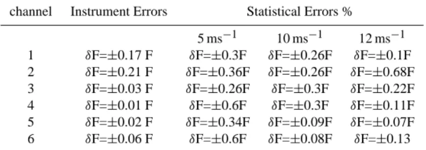
The second error analysis performed was the determina-tion of the statistical errors in the average fluxes due to the variability of the individual estimates. It is to be expected
Table 2. The Instrument and Statistical errors for each channel of the CLASP instrument as used in WASFAB 05.
channel Instrument Errors Statistical Errors %
5 ms−1 10 ms−1 12 ms−1 1 δF=±0.17 F δF=±0.3F δF=±0.26F δF=±0.1F 2 δF=±0.21 F δF=±0.36F δF=±0.26F δF=±0.68F 3 δF=±0.03 F δF=±0.26F δF=±0.3F δF=±0.22F 4 δF=±0.01 F δF=±0.6F δF=±0.3F δF=±0.11F 5 δF=±0.02 F δF=±0.34F δF=±0.09F δF=±0.07F 6 δF=±0.06 F δF=±0.6F δF=±0.08F δF=±0.13
that the statistical errors are larger than the systematic errors due to the inherent variability of turbulent flux estimates and the limited data set obtained. The statistical errors vary for wind speed and particle size covering a range from 2 to 68% however a typical error is around 30%. The statistical errors are shown in Table 2 and indicated in Fig. 6.
The results from this work conform well to the SSSFs from the literature in both magnitude and size spectral shape, for all wind speeds, and in particular to Monahan et al. (1986). One notable discrepancy is that our results indicate an in-crease in the flux with reduction in size for the two smallest size bins whereas M˚artensson et al. (2003) and Clarke (2006) both show a decrease. This size range is near the limit of the CLASP capability and extension to smaller sizes is needed to properly evaluate the spectral behaviour of the fluxes of these particles.
The variations between sea spray source functions at ferent wind speeds in Fig. 6 are likely due to the use of dif-ferent methods, with their own inherent uncertainties, and different environmental conditions other than wind speed: wave height, wave ages, coastal effects, stability of the
atmo-sphere, etc. Recent formulations have shown that u∗(Lafon
et al., 2004) or wave height (Woolf, 2005) can provide better parameterisations for the whitecap fraction, which is often used in sea spray source function formulations (e.g. Mona-han et al., 1986; M˚artensson et al., 2003).
Some of the differences may also be due to differing mea-surement heights and locations. Andreas (1998) applies to the flux at the surface and is based on Smith et al. (1993) which was developed from measurements at 14 m above the mean ocean surface on a sloping beach. It is noted that Smith et al. (1993) ruled out the possibility that these data were influenced by production in the surf zone. Andreas argues that the Smith et al. SSSF underestimates the true surface production and he suggested a correction. Similarly, Smith and Harrison’s (1998) measurements, for particles sized 1 to 15 µm, were at a nominal height of 10 m above the ocean surface and it is suggested that the actual SSSF at the sur-face as defined by Andreas (1998) may be between 1.2 to 4 times their reported function. It is noted, however, that most authors use an “effective” source height of the order of 10 m
above the mean sea surface. Andreas (2002) showed that for particles less than 2 µm in radius and for wind speeds of
up to 20 m s−1, the ratio between the flux at a measurement
height of roughly 10 m and the flux near the ocean surface, at roughly 1 m, is very small. Therefore, there is little need to correct our measurements – made 16.5 m above the surface – for height. It is worth noting that an air-sea interface source function is important for full process level knowledge but, for many processes such as the flux of particles into the mixed layer, an effective source function at the top of the constant flux layer is sufficient.
5 Conclusions
The results from the eddy covariance flux system during WASFAB show strong positive correlation between the
par-ticle fluxes and the local windspeed from 3 to 12 m s−1for
particles up to a micron in radius. The flux results compare favourably with a number of recent sea spray source func-tions from the literature across a range of wind speeds from
3 to 12 m s−1. It was not, however, viable to calculate an
in-dependent sea spray source function from this limited series of observations.
One of the main limitations with all field measurements of sea spray particles from coastal sites is that the measure-ments are typically representative of only one location and one point in time; frequently the statistics are also poor due to the limited quantities of data obtained. This limitation ap-plies here – the WASFAB field campaign lasted three weeks, but good conditions for sea spray flux measurements were obtained on only 3 days. Coastal measurement sites are gen-erally less than ideal due to effects of the surf zone – an intense local source of sea spray particles due to much in-creased wave breaking compared with the open ocean (de Leeuw et al., 2000). The long pier at Duck, combined with onshore wind conditions, provided a site well away from the effects of tides or the surf zone. The drag coefficient mea-surements made by Zappa et al. (2006) give us confidence that this site is reasonably representative of the open ocean under the conditions encountered in this study.
562 S. J. Norris et al.: EC fluxes of sea spray We have demonstrated the feasibility of making direct,
size-resolved, flux measurements of sea spray aerosol via the eddy covariance technique for the first time. Work is ongo-ing to improve the size resolution of the instrument and to make measurements in the more challenging environment of the open ocean.
Acknowledgements. The work presented in this article is part of the
PhD thesis work of Sarah Norris and was supported by TNO, The Netherlands, through the TNO OIO funds. The TNO participation in the WASFAB experiments and analysis was supported by the US Office of Naval Research, Award: N00014-96-1-0581. The Leeds participation in the WASFAB experiments was supported by the US Office of Naval Research, Unisource grant: N00014-03-1-0916. We would like to thank all the FRF personnel at Duck, particularly C. Miller, for their help and support during the WASFAB field campaign.
Edited by: W. E. Asher
References
Andreas, E. L.: Sea spray and the turbulent air-sea heat fluxes, J. Geophys. Res., 97(C7), 11 429–11 441, 1992.
Andreas, E. L.: A new Sea Spray Generation Function for Wind speeds up to 32 m s−1, J. Phys. Oceanogr., 28(11), 2175–2184, 1998.
Andreas, E. L.: A review of Sea Spray Generation Function for the Open Ocean, Atmosphere-Ocean Interactions, 1, 1-46, 2002. Anguelova, M. D. and Webster, F.: Whitecap coverage from
satellite measurements: A first step toward modeling the vari-ability of oceanic whitecaps, J. Geophys. Res., 111, C03017, doi:10.1029/2005JC003158, 2006.
Blanc, T. V.: The effects of inaccuracies in weather-ship data on bulk-derived estimates of flux, stability and sea-surface rough-ness, J. Atmos. Ocean. Tech., 3, 12–26, 1986.
Blanchard, D. C.: The production, distribution, and bacterial enrich-ment of the sea-salt aerosol, in: The air-sea exchange of Gases and Particles, edited by: Liss, P. S. and Slinn, W. G. N., D. Rei-del, Norwell, Mass, 407–454, 1983.
Blanchard, D. C. and Woodcock, A. H.: The production, concen-tration, and vertical distribution of the sea-salt aerosol, Ann. NY Acad. Sci., 338, 330–347, 1980.
Buzorius, G., Rannk, U., Makela, J. M., Vesala, T., and Kulmala, M.: Vertical aerosols particles fluxes measured by eddy covari-ance technique using condensation particle counter, J. Aerosol Sci., 29(1/2), 157–171, 1998.
Clarke, A. D., Owens, S. R., Zhou, J.: An ultra fine sea -salt flux from breaking waves: Implications for cloud condensation nu-clei in the remote marine atmosphere, J. Geophys. Res., 111, D06202, doi:10.1029/2005JD006565, 2006.
Davis, C. N.: The entry of aerosols into sampling tubes and heads, British, J. Appl. Phys., 1(2), 921–932, 1968.
de Leeuw, G., Neele, F. P., Hill, M., Smith, M. H., and Vignati, E.: Sea spray aerosol production by waves breaking in the surf zone, J. Geophys. Res., 105(D2), 29 397–29 409, 2000.
de Leeuw, G., Moerman, M., Zappa, C. J., McGillis, W. R., Nor-ris, S. J., and Smith, M. H.: Eddy Correlation Measurements of Sea Spray Aerosol Fluxes, in: Transport at the Air Sea Interface,
edited by: Garbe, C. S., Handler, R. A., and J¨ahne, B., Springer-Verlag Berlin, Heidelberg, 2007.
Desjardins, R. L., Macpherson, J. I., Schuepp, P. H., and Karanja, F.: An Evaluation of Aircraft Flux Measurements of CO2, Water
Vapour and Sensible Heat, Bound.-Lay. Meteorol., 47, 55–69, 1989.
Fairall, C. W., Kerpert, J. D., Holland, G. J.: The effects of Sea Spray on Surface Energy Transports over the Ocean, The Global Atmosphere and Ocean System, 2, 121–142, 1994.
Fairall, C. W., Banner, M., Morison, R., and Persion, W.: Depen-dence of spray flux on breaking waves, Ocean Sciences Meeting of the American Geophysical Union, Honolulu, HI, OS53F-02, 2006.
Frederickson, P. A., Davidson, K. L., and Edson, J. B.: A study of Wind Stress Determination Methods from a Ship and an Offshore Tower, J. Atmos. Ocean. Tech., 14, 822–835, 1997.
Friehe, C. A., Williams, E. R., and Grossman, R. L.: An inter-comparison of two aircraft gust probe systems, Symposium on Lower Tropospheric Profiling: Needs and Technologies, Boul-der, Colorado, American Meteorology Society, 235–236f, 1988. Gallagher, M. W., Beswick, K. M., Duyzer, J., Westrate, H., Choularton, T. W., and Hummelshoj, P.: Measurements of Aerosol fluxes to Speulder forest using a micrometeorological technique, Atmos. Environ., 31(3), 359–372, 1997.
Geever, M., O’Dowd, C. D., van Ekeren, S., Flanagan, R., Nilsson, E. D., de Leeuw, G., and Rannik, U.: Submi-cron Sea Spray Fluxes, Geophys. Res. Lett., 32, L15810, doi:10.1029/2005GL023081, 2005.
Gerber, H. E.: Relative-humidity parameterization of the navy aerosol model (NAM). Navel Research Laboratory, Washington, Report No. NRL Report 8956, 17 pp., 1985.
Haywood, J. M., Ramaswamy, V., and Soden, B. J.: Tropospheric aerosol climate forcing in clear-sky satellite observations over the oceans, Science, 238, 1299–1303, 1999.
Hoppel, W. A., Cafferey, P. F., and Frick, G. M.: Particle deposition on water: Surface sources versus upwind sources, J. Geophys. Res., 110, D10206, doi:10.1029/2004JD005148, 2005.
Hill, M., Brooks, B., Norris, S. J., Smith, M. H., Brooks, I. M., de Leeuw, G., and Lingard, J.: A novel high-temporal resolution particle spectrometer, J. Atmos. Ocean. Tech., accepted, 2007. IPCC: Climate Change 2001: The Scientific Basis, Contribution of
Working Group I to the Third Assessment Report of the Inter-governmental Panel on Climate Change, edited by: Houghton, J. T., Ding, Y., Griggs, D. J., Noguer, M., van der Linden, P. J., Dai, X., Maskell, K., and Johnson, C. A., Cambridge University Press, Cambridge, United Kingdom and New York, NY, USA, 881 pp., 2001.
Kaimal, J. C. and Finnegan, J. J.: Atmospheric Boundary Layer flows: Their Structure and Measurement, Oxford University Press, 1994.
Kiene, R. P.: Sulphar in the mix, Nature, 402, 363–364, 1999. Kristensen, L., Mann, J., Oncley, S. P., and Wyngaard, J. C.: How
Close is Close Enough when Measuring Scalar Fluxes with Dis-placed Sensors?, J. Atmos. Ocean. Tech., 14, 814–821, 1997. Lafon, C., Piazzola, J., Forget, P., Le Calve, O., and Despiau, S.:
Analysis of the Variations of the Whitecap Fraction as Mea-sured in a Coastal Zone, Bound.-Lay. Meteorol., 111(2), 339– 360, 2004.
Lewis, E. R. and Schwartz, S. E.: Sea Salt Aerosol Production –
Mechanisms, Methods, Measurements, and Models, American Geophysical Union, 2004.
Massman, W. J. and Lee, X.: Eddy covariance flux corrections and uncertainties in long term studies of carbon and energy ex-changes, Agr. Forest Meteorol., 113, 121–144, 2002.
M˚artensson, E. M., Nilsson, E. D., de Leeuw, G., Cohen, L. H., and Hansson, H. C.: Laboratory simulations and parameteriza-tion of the primary marine aerosol producparameteriza-tion, J. Geophys. Res., 108(D9), 4297, doi:10.1029/2002JD002263, 2003.
Monahan, E. C., Fairall, C. W., Davidson, K. L., and Boyle, P. J.: Observed inter-relationships amongst 10m-elevation winds, oceanic whitecaps, and marine aerosols, Q. J. Roy. Meteor. Soc., 109, 379–392, doi:10.1002/qj.49710946010, 1983.
Monahan, E. C.: Oceanic Whitecaps: Sea Surface Features De-tectable via Satellite that are Indicators of the Magnitude of the Air-sea Gas Transfer Coefficient, Proceeding of Indian Aca-demic Science (Earth Planet Science), 111, 315–331, 2002. Monahan, E. C., Spiel, D. E., and Davidson, K. L.: A model of
marine aerosol generation via whitecaps and wave disruption, in: Oceanic whitecaps, edited by: Monahan, E. C. and Mac Niocaill, G., D. Reidel Publishing Company, 167 pp., 1986.
Nilsson, E. D., Rannik, U., Swietlicki, E., Leck, C., Aalto, P. P., Zhou, J., and Norman, M.: Turbulent aerosol fluxes over the Arc-tic Ocean 2. Wind-driven sources from the sea, J. Geophys. Res., 106(D23), 32 139–32 154, 2001.
O’Dowd, C. D., Lowe, J. A., and Smith, M. H.: Coupling of sea-salt and sulphate interactions and its impact on cloud droplet con-centration predictions, Geophys. Res. Lett., 26(9), 1311–1314, 1999.
O’Dowd, C. D. and de Leeuw, G.: Marine Aerosol Production: a re-view of the current knowledge, Phil. Trans. R. Soc. A 365, 1753– 1774, doi:10.1098/rsta.2007.2043, 2007.
Reid, J. S., Jonsson, H. H., Smith, M. H., and Smirnov, A.: Evolu-tion of the Vertical Profile and Flux of Large Sea-Salt Particles in a Coastal Zone, J. Geophys. Res., 106(D11), 12 039–12 053, 2001.
Schulz, M., de Leeuw, G., and Balkanski, Y.: Sea-salt aerosol source functions and emissions, in: Emissions of Atmospheric Trace Compounds, edited by: Granier, C., Artaxo, P., and Reeves, C., Kluwer, 333–359, 2004.
Seinfeld, J. H. and Pandis, S. N.: Atmospheric Chemistry and Physics, Air Pollution to Climate Change, John Wiley and Sons, Inc., 1997.
Slinn, S. A. and Slinn, W. G. N.: Modelling of Atmospheric Partic-ulate Deposition to Natural Waters, in: Atmospheric pollutants in natural waters, edited by: Eisenriech, S. J., Arbor Science, Michigan, 23–53, 1981.
Smith, M. H. and N. M. Harrison: The Sea Spray Generation Func-tion. J. Aerosol Sci., 29(supplement 1.), S189–S190, 1998. Smith, M. H., Park, P. M., and Consterdine, I. E.: Marine aerosol
concentrations and estimated fluxes over the sea, Q. J. Roy. Me-teor. Soc., 119, 809–824, 1993.
Spiel, D. E.: On the births of film drops from bubbles bursting on seawater surfaces, J. Geophys. Res., 103(C11), 24 907–24 918, 10.1029/98JC02233, 1998.
Stull, R. B.: An introduction to Boundary layer Meteorology, Kluwer Academic, San Diego, California, 1988.
Woolf, D. K.: Parameterization of gas transfer velocities and sea-state-dependent wave breaking, Tellus, 57B, 87–94, 2005. Yelland, M. J., Taylor, P. K., Consterdine, I., and Smith, M. H.: The
use of Inertial Dissipation Technique for shipboard wind stress determination, J. Atmos. Ocean. Tech., 11, 1093–1108, 1994. Zappa, C. J., Tubiana, F. A., McGillis, W. R., Bent, J., de Leeuw, G.,
and Moerman, M. M.: Investigating wave processes important to air-sea fluxes using infrared techniques, Ocean Sciences Meeting of the American Geophysical Union, Honolulu, HI, OS13C-03, 2006.