Firm-Level Productivity and Technical Efficiency in MENA Manufacturing Industry: The Role of the Investment Climate

HAL Id: halshs-00556700

https://halshs.archives-ouvertes.fr/halshs-00556700

Preprint submitted on 17 Jan 2011

HAL is a multi-disciplinary open access

archive for the deposit and dissemination of sci-entific research documents, whether they are pub-lished or not. The documents may come from

L’archive ouverte pluridisciplinaire HAL, est destinée au dépôt et à la diffusion de documents scientifiques de niveau recherche, publiés ou non, émanant des établissements d’enseignement et de

Firm-Level Productivity and Technical Efficiency in

MENA Manufacturing Industry: The Role of the

Investment Climate

Tidiane Kinda, Patrick Plane, Marie-Ange Véganzonès-Varoudakis

To cite this version:

Tidiane Kinda, Patrick Plane, Marie-Ange Véganzonès-Varoudakis. Firm-Level Productivity and Technical Efficiency in MENA Manufacturing Industry: The Role of the Investment Climate. 2011. �halshs-00556700�

CERDI, Etudes et Documents, E 2008.19

Document de travail de la série Etudes et Documents

E 2008.19

Firm-Level Productivity and Technical Efficiency in MENA

Manufacturing Industry: The Role of the Investment Climate

by Tidiane Kinda* Patrick Plane** and Marie-Ange Véganzonès-Varoudakis** 36 p.

* CERDI, Université d’Auvergne, France

Abstract

This paper investigates the relationship between firm-level productivity and investment climate (IC) for a large number of countries (23) and manufacturing industries (8). We first propose three measures of firms’ productive performances: Labor Productivity (LP), Total Factor Productivity (TFP), and Technical Efficiency (TE). We reveal that enterprises in MENA perform in average poorly, compared to other countries of the sample. The exception is Morocco, whose various measures of firm-level productivity rank close to the ones of the most productive countries. We show at the same time that firms’ competitiveness in MENA is handicapped by high Unit Labor Cost, compared to main competitors like China and India. The empirical analysis also reveals that the investment climate matters for firms productive performances. This is true (depending on the industry) for the quality of a large set of infrastructures, the experience and level of education of the labor force, the cost and access to financing, as well as to a lower extent, different dimensions of the government-business relation. These findings bear important policy implication by showing which dimension of the investment climate could help manufacturing firms in MENA to be more competitive on the world market.

Firm-Level Productivity and Technical Efficiency in MENA

Manufacturing Industry: The Role of the Investment Climate

1- Introduction

The revival of interest in economic growth has renewed the question of the differences in productivity among countries and regions. Productivity, in the form of technical progress and production efficiency, is actually seen as the major source of economic growth and convergence of the economies. This question has justified that a growing research has focused on the manufacturing industry, as the place of innovation and the engine of growth. Productivity in the manufacturing industry is also central to international competitiveness, as developing countries face the increasing pressure of globalization. High productivity gains have been seen as a powerful means of improving export capacity and diversifying the economy. The persistence of productivity differences across countries, regions and firms, however, don’t find any justification in the present situation of globalization characterized by capital mobility and diffusion of technology. These differences have to be explained by factors which are specific to each country and region. It is in this context that a new branch of the literature has explored the question of the differences in the investment climate, as a major factor contributing to the differences in productivity1. It is this direction that we have also chosen, to explain MENA deficient economic performances.

Understanding the factors that affect industrial performances bears important policy implication in the case of MENA, who does not benefit from a diversified economy and a substantial manufacturing export capacity. Although MENA countries are, in average, defined as middle income countries, economic performance in the region has most of the time been disappointing. This has been the case of growth and investment for more than three decades22. Attractiveness of FDI has also been weak, as well as competitiveness and exports of manufacturing33. In fact, MENA competitiveness has constantly been affected by poor exchange rate policies and insufficient economic reforms. But other factors, such as the investment climate, can surely explain the low productivity and the high production costs at the firm level, as various studies point out MENA investment climate deficiencies44. These deficiencies have been reported as participating in the slow economic activity in the region55.

The World Bank Investment Climate (ICA) surveys collect data on inputs and outputs, as well as on various aspects of the investment climate at the firm level. ICA surveys produce both subjective evaluations of obstacles, as well as other more objective information on the themes of infrastructure, human capital, technology, governance, and financial constraints. These standardized surveys of large, random samples of firms from different sectors permit comparative measures of firms’ productive performance. They also provide information to estimate the contribution of investment climate to these performances. The ICA surveys can thus be seen as an instrument for identifying key obstacles to firms’ productivity and competitiveness. They can be used as a support to

policy reforms for an increased economic growth. The objective of this paper has been to help progress in that direction.

Drawing on the World Bank firm-surveys, this paper analyses the relationship between investment climate and firm-level productivity for a large number of countries (23 among which 5 MENA countries, see list of countries in Annex 1) and manufacturing industries (8)6. We first propose different measures of firms’ productive performances by industry, such as Labor Productivity (LP), Total Factor Productivity (TFP), and Technical Efficiency (TE) using a production frontier approach. These indicators are compared with each others, as well as across countries in order to position MENA manufacturing firms amongst a wide range of firms from other regions. We reveal that enterprises in MENA perform in average poorly, compared to other countries of the sample. The exception is Morocco, whose various measures of firms’ productive performance always rank close to the ones of the most productive firms in the sample. An originality of our approach has been, as well, to generate a few composite indicators of investment climate using Principal Component Analysis (PCA), which summarizes well the key dimensions of the investment climate. This has also allowed tackling the problem of multicolinearity when explaining firm productive performances with a wide range of correlated IC variables. We define four axes of the investment climate: the Quality of Infrastructure (Infra), the Business-Government Relations (Gov), the Human Capacity (H), and Financing Constraints (Fin). We use, as well, city-sector averages to reduce the potential endogeneity problem underlying the investment climate (IC) variables. The analysis finally shows that investment climate matters for firms’ productive performances. This has been done by estimating an efficiency function explaining firm-level productivity for each of our 8 manufacturing industries.

The paper is organized as follows. The second section introduces different concepts of firm-level productivity and discusses the advantages and limits of the different measures. Section three presents briefly the investment climate (ICA) surveys data and summarizes their main limitations. The fourth section presents and compares across countries our different estimations of firms’ productive performances by industry. The fifth section introduces and categorizes the investment climate indicators used in the empirical analysis, and calculates our four broad IC indicators. In the sixth section, we estimate to which extend the investment climate constraints firms productive performances. The last section concludes.

2- Measures of Firm-Level Productivity: Methodological Aspects

The first challenge is to measure firms’ productive performance in a relevant way. We propose different approaches and measures. We first consider a non parametric model of productivity, which consists in calculating productive performances without estimating a production function. Non parametric measure of productivity constitutes a simple and already meaningful way of assessing for example Productivity of Labor (LP) and Total Factor Productivity (TFP). Another way has been to calculate firms’ productive performance from a parametric production frontier. This more sophisticated methodology

allows to identify the most efficient firms of the sample and to compare MENA firms’ performances to them.

2.1- Non Parametric Measures of Productivity and Unit Labor Cost

Productivity can be easily calculated as the ratio of an output to a specific factor of production, labor being the main input whatever the industrial sector. We can also consider all the relevant factors of the production technology. We then refer to the Total Factor Productivity (TFP). In this paper due to the limited time dimension for the production factors, two or three years at best, and no time dimension about the Investment Climate Assessment determinants (ICA), we only refer to productivity levels. Our analysis focuses on comparisons of firm-level productivity among enterprises, industries and countries7.

In the empirical analysis, we first discuss Labor Productivity (LP). This indicator gives an idea of firm productive performance. It has the advantage not to be affected by the error in measurement of the capital stock. However, the technology is only partially described and then the productivity suffers from an omitted variable. Productivity of Labor can be complemented by calculations of a Unit Labor Cost defined as the ratio of firm average wage to firm labor productivity. This indicator allows comparisons of the organizational competitiveness across countries. In addition, firm productive performance can also be biased by the choice of the exchange rate when converting production into US$. This is less the case when the TFP is estimated. The same rate applies to the output (Y) at the numerator but also to the intermediate consumption (ICO) and the capital stock (K) at the denominator, under the form of a weighted average of these inputs. Under the hypothesis of constant returns to scale, (i.e., perfect competition for goods but also for factors that are remunerated at their marginal productivity), weights of Intermediate Consumptions (ICO) and of Labor (Wages, W) are calculated as the ratio of the cost of these factors to the Total Cost of Production including profit (Y). The contribution of Capital (K) is then calculated as the complement to one. The advantage of this approach based on the Solow residuals is that it does not require the inputs to be exogenous or the inputs elasticity to be constant. The disadvantage is that two hypotheses have to hold: constant returns to scale and competitive input markets. Another limitation can be seen in the fact that productivity being calculated as the residual of the production function, it is considered as a random variable, what makes difficult to justify that some exogenous factors can explain productive differences.

1i 2i (1 1i 2i) i i i i i Y TFP L ICOω ω K −ω −ω = (1) 1 , 2 i i i i i i W ICO Y Y ω = ω = (2)

2.2- Parametric Production Functions and Production Frontiers

In the parametric approach, TFP is calculated as the residual of an estimated production function, thus relaxing the hypotheses of constant returns to scale (but not automatically of productivity as a random variable). Various hypotheses can be done regarding the technology of production. The Cobb Douglas and the Translogarithmic production functions are the most commonly used. Although both present good mathematic properties, the elasticities of the production to the inputs are easy to read and to interpret with the Cobb Douglass technology. In the case of a parametric production function, production is derived from the optimization problem of firms, which maximize current and expected profits by equating production prices to their marginal costs. This hypothesis does not permit any waste of resources or organizational weaknesses. The production frontier approach, however, allows for non optimal behaviors of the firms. Enterprises can be positioned in regard to the most efficient firms that define an empirical production frontier. Firm-level Technical Efficiency (TE) can then be defined as the firms’ productivity gap (or efficiency gap) to the “best practice”, the empirical practice of firms which are located on the production frontier.

In the stochastic model, the likelihood estimation method is typically applied to estimate a “composite” error term which is split into two uncorrelated elements. The first term (v), which is a random variable, represents the external shocks to the firm. These shocks, independent and identically distributed, follow a normal distribution, with zero average and σ² standard deviation. The second term represents the Technical Efficiency (-u). In our case we will suppose that u follows a truncated normal distribution8. In this specification, firms’ productive performances are not assimilated to a random variable and can then be explained by exogenous factors. The interest of this approach can also be seen in the fact that TEs have a relative form, firm productivity being compared to or benchmarked by the most efficient ones across countries and regions.

i i i i f x u v y = ( ,β)− + (3) With - y: Production - x: Production factors

- β : Parameters of the equation - v : External shocks

- u : Technical Efficiency (TE) - i: Firm index

2.3- Explaining Technical Efficiency

A complementary approach, when having calculated Technical Efficiency (TE), is to explain the reasons for firms’ diverse performances. Firms’ inefficiency can be explained by “exogenous” factors which affect either the technology of production, or the firm’s ability to transform inputs into outputs. In the literature, these factors have been estimated in two different ways. A simple method consists in estimating the stochastic production

frontier, and in regressing the residuals of the estimation (the Technical Efficiency, TE) on a vector of explanatory factors (z). This method is called the “Two Steps” procedure. Different estimation procedures can be used. The simplest way is to run an OLS regression. Another possibility is to apply a Tobit model, in order to address the question of the distribution of the efficiency. The “Two Steps” procedure presents, however, several limitations. There is an identifying problem in separating the Technical Efficiency (TE), from the production frontier. When any of the production frontier inputs (x) is influenced by common causes affecting efficiency, there is a simultaneity problem (see Marschak and Andrews, 1944; Griliches and Mairesse, 1995). In general, one should expect that the Technical Efficiency term (TE) is correlated with the production frontier inputs (x). In this case, due to the omission of important explanatory variables, the likelihood estimation of the stochastic production frontier is biased.

In fact, a relatively new branch of the literature proposes to estimate the production frontier and the factors explaining inefficiency at the same time. This is the “One Step” procedure. In this case, the parameters of the equation (here β and δ) are simultaneously estimated by the likelihood estimation method. The stochastic version of the model can be written: i i i i i f x z u v y = ( , ,β,δ)− + (4) With - y: Production - x: Production factors

-z: Factors explaining Technical Efficiency - v : External shocks

- u : Technical Efficiency - β / δ: Parameters of the equation - i: Firm index

3- The ICA Firms Surveys: Data Limitations

The World Bank Investment Climate (ICA) surveys collect data on inputs and outputs, as well as on a large variety of quantitative and qualitative (perception-based) indicators of the investment climate. In building the database, we have tried to incorporate as much information as possible. We have integrated in our sample 23 countries surveyed at the time our empirical work started (see list of countries in Annex 1)9. These countries participate in the five main regions of the developing world: Sub-Saharan Africa (AFR), East Asia (EAS), South Asia (SAS), Latin America and the Caribbean (LAC), Middle East and North Africa (MENA). In this sample, MENA is represented by 5 countries: Algeria (2002), Saudi Arabia (2005), Lebanon (2006), Morocco (2000, 2004) and Egypt (2004, 2006)10. Syria (2003) and Oman (2003) had to be removed from the sample because of a very low rate of answer to the questionnaire. By broadening the initial sample to a large number of countries from different regions, we have intended to compare MENA performances to the ones of emerging countries which appears as major competitors on the world market: China (2002) and India (2000, 2002), in particular.

To estimate firm-level productivity, a population of almost 20,000 firms, coming from 13 manufacturing industries was initially considered. This sample had to be reduced due to various limitations particularly the lack of the production technology variables and the necessity of a cleaning up when figures proved to be poorly transmitted or recorded. Some industries as well had to be merged, due to insufficient observations. In fine, 12 414 enterprises (3073 for the MENA region) regrouped in eight industries were retained when estimating production frontiers (see Annex 2)11. As for inputs and output, investment climate (IC) variables are subject to measurement errors. In the surveys, some firms did not report the full range of investment climate measures. Other firms reported numbers that were not credible. This is also due to the fact that most of investment climate factors are qualitative variables of perception, thus allowing answers to vary depending on the firms, the regions or the countries. Our choice has been to keep as many firms as possible, providing sufficient information on a wide range of investment climate variables. Once outliers and incomplete observations are removed, 5002 observations were left, among which 1483 for the MENA region, what represent 34% of MENA initial population and 30% of the total number of enterprises with IC variables (see Annex 2)12. The IC variables considered here are the ones that we use to explain firms’ Technical Efficiency (TE) (see sections 5 and 6).

Another question relates to the endogeneity of the IC variables, due to the qualitative nature of investment climate factors. This is particularly true for perception variables (such as obstacles to operation) for which firms are asked to position their answer on a given scale13. The perception of the scale might be different across firms, industries, regions and countries. Besides, when answering the questions on their investment climate, firms may be influenced by the perception they have of their own productivity and may attribute their inefficiencies to external factors. High-performing firms, as well, may be proactive in reducing their investment climate constraints, for example by working with the authorities to limit inspections or secure more reliable power supply. In the empirical part, we assume this endogeneneity and use appropriate estimation techniques to evaluate the impact of the investment climate on the firms’ productive performances. We measure in particular IC variables as city-sector averages of firm-level observations14. This also helps to mitigate the effects of missing observations for some firms. Actually, if we take each investment climate indicator at the firm level, we end up with a smaller sample of observations in which all indicators are available15.

Exchange rate constitutes another source of uncertainty which may lead to over or under evaluate firms’ productive performances. This rate is used to convert production and production factors into US dollars. Several exchange rates can be chosen to calculate and compare firm-level productivity across countries. In this study, we considered the current market rate in US dollars which has the interest to be the rate that firms use for their economic calculations16.

4- Firm-Level Productivity: MENA Performance Gap

In this section, we present our three measures of firm-level productivity: Productivity of Labor (LP), Total Factor Productivity (TFP) and Technical Efficiency (TE). The data have been pooled across the 23 countries of our sample. Firm-level productive performances are calculated for each of the 8 industries. Differences and similarities across countries have been analyzed. A pattern of generally low productive performances is observed in the MENA region, with however some countries showing better results.

4.1- Firm-level Productivity of Labor and the Unit Labor Cost

Firm-level Productivity of Labor (LP) is estimated as the ratio of firms’ Value Added to the Number of Permanent Workers. Value Added is calculated as the difference between Total Sales and Total Purchase of Raw Material -- excluding fuel17. It is assumed that firms are price takers and purchase raw material at world price. This assumption is reasonable for the industries which are competitive. Thus, the dollar value of raw material and the dollar value of output can be compared across countries.

Equation is as follows:

LP i, j = Y i, j /L i, j (5)

With

- Yi, j: Value Added.

- L i, j : Number of Permanent Workers

- i / j: Enterprise and country index respectively.

Table 1 displays the averages Labor Productivity (LP) while table 2 reflects the relative Unit Labor Cost. For each country, average productivity (Labor productivity and Unit Labor Cost) is expressed in percent of the level of the country with the most performing firms (or the country with the lowest Unit Labor Cost). The analysis reveals a relatively stable ranking of countries. South African and Brazilian firms perform -- in average and in most industries -- the best. This result is consistent with the relatively high incomes in the two countries (2710 and 2780 dollars per capita respectively, see World Bank, 2005). Morocco (2004)’s firms also participate in the best performances of the sample, especially in Metal & Machinery Products, Chemical & Pharmaceutical Products, Leather, and Agro-Processing.

Table 1. Firm-Level Relative Productivity of Labor

(Country average, in % of the country with the most productive firms)

Country* Textile Leather Garment

Agro Processing Metal & Machinery Products Chemic & Pharm Products Wood & Furniture Non Metal & Plastic Materials South Africa (2003) 52 100 100 94 97 87 100 Brazil (2003) 100 100 50 50 66 100 38 Morocco (2004) 54 80 54 79 100 91 66 Morocco (2000) 56 94 55 85 48 63 57 Saudi Arabia (2005) 77 92 100 Ecuador (2003) 58 91 80 48 50 54 42 66 El Salvador (2003) 71 59 55 35 28 51 46 China (2002) 52 69 45 31 Thailand (2004) 62 62 45 40 31 43 Guatemala (2003) 43 64 31 26 36 33 48 India (2002) 35 66 53 21 22 17 Honduras (2003) 56 50 29 23 39 21 26 India (2000) 39 48 28 24 Pakistan (2002) 40 35 49 22 17 Tanzania (2003) 35 20 Philippines (2003) 32 32 14 Algeria (2002) 27 21 19 19 31 Bangladesh (2002) 18 53 16 9 11 Nicaragua 2003 13 38 26 17 13 17 16 21 Sri Lanka (2004) 13 27 9 17 28 Zambia (2002) 16 13 24 18 Ethiopia (2002) 11 20 20 10 10 Egypt (2006) 14 15 14 12 16 11 10 13 Egypt (2004) 15 20 14 9 11 11 11 11 Lebanon (2006) 11 17 8 7

Note : * Ranking is from countries with the most productive firms to the ones with the least productive firms.

Source. Authors’ calculations

As far as other MENA countries are concerned, the ranking remains also rather stable. Egyptian and Lebanese’s firms are systematically among the least performing in all industries (although Morocco and Egypt have the same GDP per capita, at around 1300 US dollars in 2003). In Algeria, firm-level Productivity of Labor (LP) ranks an intermediate position, close to India in Agro-Processing and Chemical& Pharmaceutical Products, but behind in Textile and Metal & Machinery Products (firms’ performances are always lower than in China). Moroccan’s firms remain the most performing ones in MENA, with levels of Labor Productivity (LP) far ahead from the two Asiatic giants (China and India), and close to the most productive firms/countries of the sample18.

Table 2. Firm-Level Relative Unit Labor Costs

(Country average, % of the country with the highest unit cost)

Country* Textile Leather Garment

Agro Processing Metal & Machinery Products Chemic & Pharm Products Wood & Furniture Non Metal & Plastic Materials El Salvador (2003) 52 100 100 85 100 63 87 Nicaragua (2003) 100 72 80 87 88 100 92 79 Guatemala (2003) 64 83 100 79 87 89 74 Algeria (2002) 73 89 89 96 100 Philippines 2003) 66 92 83 South Africa (2003) 86 97 74 80 88 69 64 Morocco 2004) 81 79 91 75 75 76 60 Honduras (2003) 36 78 88 76 63 96 86 Egypt (2004) 51 66 77 77 55 86 100 57 Egypt (2006) 60 86 76 71 46 80 92 51 Saudi Arabia (2005) 89 59 55 Lebanon (2006) 55 53 61 92 Morocco (2000) 62 62 84 60 58 66 62 Zambia (2002) 46 75 48 88 Brazil (2003) 48 54 72 68 56 49 65 Sri Lanka (2004) 86 64 71 39 32 Bangladesh (2002) 49 34 60 69 55 Ethiopia (2002) 71 25 45 56 55 Ecuador (2003) 48 59 52 50 42 32 62 53 Thailand (2004) 42 56 49 35 52 34 China (2002) 39 41 54 38 Pakistan (2002) 31 41 33 47 51 India (2000) 36 38 37 46 India (2002) 32 27 35 42 35 44 Tanzania (2003) 33 31

Note : * Ranking is from countries with the most expensive labor to the ones with the least expensive one.

Source. Authors’ calculations

This relative efficiency of some MENA countries, however, is not sufficient to understand the capacity of these countries to promote industrial and export activities. Remuneration of labor is an important factor which should be in line with productivity. By combining information on Productivity of Labor (LP) and the cost of the labor input, the Relative Unit Labor Cost gives an idea of the competitiveness. Table 2 presents some information on the subject. It is worth noticing that the Unit Labor Cost in MENA is one of the highest of our sample of countries. This is particularly true in Algeria and Egypt – countries where firm-level Productivity of Labor (LP) is among the lowest – but also in Morocco and to some extend in Lebanon. In MENA, the Unit Labor Cost tends to be higher than in the majority of Asian economies (India, China, Sri Lanka, Bangladesh and Thailand).In China and India, salaries (around 100 US dollars per month for unskilled workers) are far lower than in Morocco (more than the double). In the labor intensive sectors of Textile and Garments, cost of labor is two to two and a half time higher in

Egypt and Morocco than in India. This situation is all the most important to address, if MENA wants to compete in the world market. If not, MENA will continue to suffer from the faster technological innovation in Asia where wages remain low.

4.2-Firm-Level Total Factor Productivity

In this section, firm-level Total Factor Productivity (TFP) is calculated from a non parametric relation. Production factors include Labor (L) and Capital (K). Same hypotheses and definitions as before apply to input and output variables.

TFP i, j = Log(Y i, j) – α Log (K i, j) – β Log (L i, j) (6)

With

- Y i, j: Value Added

- L i, j: Number of Permanent Workers

- K i, j: Gross Value of Property, Plant and Equipment

- β: Ratio of Total Wages (W) to Total Production Cost (Y). - α = 1- β

- i / j: Enterprise and country index, respectively

Table 3 presents the firm-level relative TFP by industry under the reasonable assumption that a sector-based technology leads to a more homogeneous production function. As for Productivity of Labor, results are presented in percent of the average TFP of the most performing country. Conclusions are quite similar than for Productivity of Labor. A first conclusion concerns the ranking of the most performing countries. As previously, South Africa and Brazil present, in most industries, the most performing firms. These countries are again followed by Morocco, which firms’ performances are quite good in most industries. When compared to Brazil, Moroccan firms show a TFP gap of 10 to 30 percent depending on the industry, what is less than the revenue gap between the two countries (47 %, or 38.5% in PPP). As far as MENA is concerned, ranking is also quite similar than for Productivity of Labor (LP). As previously, Egypt and Lebanon rank at the bottom of the sample and Algeria stays in an intermediate position. TFP calculations thus confirm the productivity gap assessed through Productivity of Labor19.

Table 3. Firm-Level Relative Total Factor Productivity

(Country average, in % of country with the most productive firms)

Country* Textile Leather Garment

Agro Processing Metal & Machinery Products Chemic & Pharm Products Wood & Furniture

Non Metal & Plastic Materials South Africa(2003) 88 100 100 91 82 100 100 Brazil (2003) 100 100 87 100 100 100 91 Morocco (2000) 80 81 79 79 70 90 71 Thailand (2004) 70 90 75 73 78 82 Morocco (2004) 73 64 77 77 70 79 80 Saudi Arabia(2005) 70 68 81 Ecuador (2003) 69 74 76 73 75 72 78 64 El Salvador (2003) 76 70 66 64 61 69 76 Philippines (2003) 64 77 65 Algeria (2002) 65 44 59 66 76 Honduras (2003) 61 72 55 57 84 50 54 Guatemala (2003) 65 67 54 62 56 54 73 India (2000) 67 63 58 58 China (2002) 59 58 56 45 Zambia (2002) 58 52 55 52 Pakistan (2002) 55 58 56 54 48 India (2002) 59 61 49 54 51 50 Tanzania (2003) 55 53 Sri Lanka (2004) 41 51 61 51 56 Bangladesh (2002) 51 46 57 50 44 Nicaragua (2003) 49 51 45 47 42 50 44 52 Ethiopia (2002) 51 34 46 49 36 Lebanon (2006) 35 39 40 37 Egypt (2004) 41 36 35 39 34 33 36 43 Egypt (2006) 37 30 33 41 34 34 31 38

Note: * Ranking is from countries with the most productive firms to the ones with the least productive firms.

Source: Authors’ calculations

4.3- Firm-Level Technical Efficiency

Firm-level Technical Efficiency is based on the likelihood estimation procedure. As seen in section 2.2., this method allows splitting the error term into two independent factors: the error term (v), which follows a normal distribution, and the technical efficiency (u), which obeys a truncated normal distribution. The technology of production explains the Value Added (Y) by the Capital (K) and the Labor (L). Same hypotheses and definitions as before apply to input and output variables.

Log(Y i, j) = α Log (K i, j) + β Log (L i, j) + dum i, −ui, j +v i, j (7)

With:

- Y i, j: Value Added

- K i, j: Gross Value of Property, Plant and Equipment

- dum j: Country-dummy variables

- α, β: parameters of the equation - vi, j: Error term

- ui, j: Technical Efficiency (TE).

- i / j: Enterprise and country index respectively.

A production frontier has been estimated for each industry. This leads to more homogeneous production frontiers and makes it easier to attribute the residual to differences in efficiency. Differences in coefficients of capital and labor have justified this choice; against an alternative assumption consisting in estimating the same production frontier with specific sector-based dummies (see Table 4).

Table 4 presents the estimation results. In most industries, the sum of the coefficients relative to labor and capital inputs is close to one. It is a little bit higher for some sectors than can be suspected to face investment indivisibilities. In comparison with other sectors, Textile is probably the most exposed to the competition and the production technology does not reject this hypothesis. For all industries, the coefficients are statistically significant at the 99% level of confidence

Table 4: Estimations of Stochastic Production Frontiers

Dependant Variable: Value Added Independent

Variables

Textile Garment Leather Agro Processing Metal & Machinery Products Chemic & Pharm Products Non Metal & Plastic Materials Wood & Furniture Log (labor) 0.659 0.811 0.826 0.695 0.877 0.673 0.886 0.941 (30.53)*** (42.69)*** (20.20)*** (31.22)*** (33.21)*** (22.21)*** (22.35)*** (29.18)*** Log (capital) 0.354 0.260 0.277 0.404 0.289 0.444 0.281 0.228 (24.87)*** (20.96)*** (11.00)*** (28.62)*** (18.52)*** (22.89)*** (13.54)*** (12.79)*** Intercept 2.007 1.350 1.419 1.863 1.716 2.065 1.419 1.644 (18.94)*** (9.22)*** (9.81)*** (13.99)*** (15.61)*** (15.39)*** (9.73)*** (11.51)*** σ_²u 0.33 0.22 0.80 0.73 1.12 0.39 1.30 0.79 σ_² 0.99 0.92 1.40 1.47 1.76 1.13 1.86 1.19 σ_{²u/ σ²} 0.33*** 0.24*** 0.57*** 0.50*** 0.64*** 0.35*** 0.70*** 0.66*** (6.17) (3.00) (6.33) (8.17) (12.80) (5.00) (10.00) (13.20) Observations 2011 2800 634 2190 1622 1274 907 1033

Note: * Significance level 10 %; ** 5 %; *** 1 %. Z statistics are into brackets. Regressions include country-dummy variables. Source: Authors’ calculations

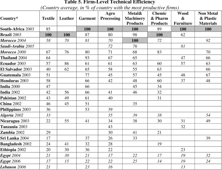
Table 4 also specifies the percentage of the residual explained by the Technical Efficiency (TE). In all industries, the efficiency term accounts for a significant part of the total residuals and is statistically significant at 99%. This result justifies the production frontier model, against the production function approach. In this model, TE explains from 24% of the error term in Garment to 70% in Non Metallic & Plastic Materials. TEs are distributed in an interval of 0 to 1 (1 is the value of the sector’s most efficient firms). In Table 5, TEs are in percent of the average TE of the most performing country. In average,

our results for Technical Efficiency (TE) are close to the ones obtained for the non parametric TFP under the hypotheses of constant returns to scale. The ranking of countries, in particular, remains unchanged. Only in Garment and Leather, Moroccan’s firms are surpassed by Thailand and Ecuador respectively. Ranking of MENA countries, as well, is unchanged.

Table 5. Firm-Level Technical Efficiency

(Country average, in % of country with the most productive firms)

Country* Textile Leather Garment

Agro Processing Metal& Machinery Products Chemic & Pharm Products Wood & Furniture Non Metal & Plastic Materials South-Africa 2003 85 100 100 100 89 100 100 Brazil 2003 100 100 87 80 98 100 62 Morocco 2004 58 70 81 70 100 72 92 Saudi-Arabia 2005 72 76 81 Morocco 2000 67 76 80 71 68 83 70 Thailand 2004 64 93 67 65 47 66 Ecuador 2003 57 86 61 61 63 60 57 63 El Salvador 2003 40 62 65 58 55 63 66 Guatemala 2003 51 77 45 57 45 48 67 Honduras 2003 58 66 42 48 60 37 48 India 2000 47 66 45 34 India 2002 42 56 66 41 46 32 Pakistan 2002 43 49 61 40 31 China 2002 46 45 51 35 Philippines 2003 36 53 39 Algeria 2002 33 35 39 38 54 Nicaragua 2003 22 55 41 34 38 30 31 49 Tanzania 2003 43 32 Zambia 2002 29 30 41 21 Sri Lanka 2004 17 37 26 33 39 Bangladesh 2002 24 41 32 28 19 Ethiopia 2002 20 30 36 22 23 Egypt 2004 21 30 21 17 22 17 19 32 Egypt 2006 17 15 22 22 25 14 19 24 Lebanon 2006 21 23 16 13

Note : * Ranking is from countries with the most productive firms to the ones with the least productive firms.

Source. Authors’ calculations

Annex 3 displays, by industry, the Spearman coefficients of correlation of our three measures of firm-level productivity. All coefficients are highly significant and show a high degree of correlation between the different measures. This is the case in all industries, but more specifically in Wood & Furniture, Non Metallic & Plastic Materials, and Metal & Machinery Products (after Agro-Processing, Chemicals & Pharmaceutical Products, Leather, and Textile). Beyond the proximity of the results whatever the method we use, to what extent can we impute the variance of the TEs to some factors proceeding of the investment climate?

5- Assessing the Investment Climate of the Manufacturing Industries

The World Bank Investment Climate (ICA) surveys provide information on a large number of investment climate (IC) variables -- in addition to general information on firms’ status, productivity, sales and supplies. These IC variables are classified into 6 broad categories: (a) Infrastructures and Services, (b) Finance, (c) Business-Government Relations, (d) Conflict Resolution/Legal Environment, (e) Crime, (f) Capacity, Innovation, Learning, (g) Labor Relations.

In the surveys, there are multiple indicators that cover a similar theme. Within the same theme, the correlation between indicators is quite high. One solution applied in some studies has been to restrict the analysis to a limited number of indicators and accept the potential omitted variable bias. This also poses the question whether the IC variables used provide a representative description of the investment climate and whether strength of result is due to the particular selection of variables. Another solution to overcome these problems consists in generating a few composite indicators. Because we intend to determine which investment climate variables are more detrimental to firm performances, we tried to take into consideration an as large as possible set of ICvariables which are not typically used in the literature. Since these variables are likely to be correlated, we applied Principal Component Analysis (PCA) to produce a limited number of composite indicators20.

Based on the ICA surveys, we defined the investment climate by four broad categories: Quality of Infrastructure (Infra), Business-Government Relations (Gov), Human Capacity (Human), and Financing Constraints (Finance). As seen in section 3, our choice of indicators has been restricted by several data limitations. This is also why we have not been able to cover all aspects initially developed in the surveys. Indicators have been selected on the bases of being available for as many countries as possible, as well as on capturing the different key dimensions of the investment climate. Besides, we have tried to complete as much as possible the qualitative (perception-based) IC indicators by quantitative information, in order to get a better picture of the investment climate in each industry.

The Quality of Infrastructure indicator (Infra) has been defined by six variables: Obstacle for the operation of the enterprise21 caused by deficiencies in (a) Telecommunications, (b) Electricity, and (c) Transport; (d) The presence of a firm Generator, (e) and the percentage of electricity coming from that source; the possibility for enterprise to access to (f) E-mail or (g) Internet. Infrastructure deficiencies constitute an important constraint to private sector development in developing countries (see World Bank, 1994). In the literature, deficiency in infrastructure is seen as a burden for enterprises operations and investments. Infrastructures are considered, as well, as a complementary factor to other production inputs. In particular, infrastructure stimulates private productivity by raising profitability of investment22. Furthermore, infrastructure also increases firms’ productive performances by generating externalities across firms, industries and regions23.

The Business-Government Relations indicator (Gov) includes three to six variables (depending on the industries): Obstacle for the operation of the enterprise caused by (a) Tax Rate, (b) Tax Administration, (c) Customs and Trade Regulations, (d) Labor Regulation, (e) Business Licensing and Operating Permits, and (f) Corruption. We suppose that this indicator illustrates the capacity of the government to provide an investment-friendly environment and reliable conditions to the private sector. Corruption is seen as having an adverse effect on firms’ productive performances. This fact is well documented and often described as one of the major constraints facing enterprises in the developing world (see the World Bank, 2005). Corruption increases costs, as well as uncertainties about the timing and effects of the application of government regulations (see Tanzi and Davooli, 1997). Taxation and regulations have also a first order implication on firms’ costs and productivity. Although government regulations and taxation are reasonable and warranted in order to protect the general public and to generate revenues to finance the delivery of public services and infrastructures, over-regulation and over-taxation deter productive performances by raising business start-up and firms’ operating costs.

The Human Capacity indicator (Human) is represented by three to four variables: Obstacle for the operation of the enterprise caused by deficient (a) Skill and Education of Available Workers; (b) Education level24 and (c) Years of Experience of the Top Manager; (d) Training of the Firm’s Employees. Human capital constitutes an essential factor of firms’ productive performance, stimulating capital formation by raising firms’ profitability. Human capital is also at the origin of positive externalities25. Because skilled workers are better in dealing with changes, a skilled work force is essential for firms to manage new technologies that require a more efficient organizational know-how (see Acemoglu and Shimer, 1999). New technologies generally require significant organizational changes, which are better handled by a skilled workforce (see Bresnahan, Brynjolfsson and Hitt, 2002). Human capital gives also the opportunity to the enterprises to expand or enter new markets.

The Financing Constraints indicator (Finance) consists of three variables: Obstacle for the operation of the enterprise caused by: (a) Cost, and (b) Access to Financing; (c) Access to an Overdraft Facility or a Line of Credit. Access to (and cost of) financing represent major determinant(s) of firms’ productive performance. Access to financing allows firms to finance more investment projects, what leads to an increased productivity through higher capitalistic intensity and technical progress embodied in the new equipments. Besides, financial development has a positive effect on productivity as a result of better selection of investment projects and higher technological specialization through diversification of risk. A developed financial system creates more profitable investment opportunities by mobilizing and allocating resources to the most profitable projects (see Levine, 1997).

The analysis usually treats the investment climate indicators as exogenous determinants of firms’ performance. As seen in section 3, however, this is not always the case. In order to address this issue, we have measured investment climate variables as city-sector

averages of firm-level observations. This has helped, as well, to increase the number of observations by integrating in the sample firms for which information is insufficient. All four aggregated indicators have been generated at the branch level, thus defining in each country the specific investment climate of each industry. This has implied to produce 32 aggregated indicators (four indicators for each of the eight industries) by applying Principal Component Analysis (PCA)26. For “Infrastructure” and “Business-Government Relations”, we have measured the initial variables as city-sector averages. For Human Capacity and Financing Constraints, however, the initial indicators having been interpreted as specific to each firm, information has been kept at the firm level (except for the variable “Skill and Education of Available Workers”) .

6- Investment Climate

and Firm-Level Productivity: Is there a Link?

In global economy, where technology diffuses rapidly and capital is mobile, the persistence of disparities in levels of productivity can be explained by differences in the investment climate. What determinants of productivity cause producers in one country to be more efficient than those in competing countries? Where should reform efforts be targeted to have the greatest impact on productivity? We link the investment climate to firm productive performance and identify the dimensions that account for cross-country differences in productivity. In this section, we estimate two variants of the same model. We show that our results are unambiguous and robust to the different specifications. All coefficients have been estimated by using the one step procedure, as discussed before. In other words, we simultaneously identify the production frontiers and the factors contributing to firms’ Technical Efficiency (TE)27.

6.1- Common Model with Individual Indicators of Investment Climate

Our empirical model considers a same representation for all industries. This model is estimated at the branch level, thus allowing the coefficients to vary across branches. We explain the Technical Efficiencies (TE) by regressing the logarithm of the production factors (capital and labor), as well as various plants characteristics and investment climate variables, on the logarithm of the firms’ value added. At this first stage of investigation, we use initial IC variables before aggregation. The model is as follows:

ln(y i,j) = c i + ά1 ln(l i,j) + ά2 ln(ki,j) +β Sizei,j + γ Foreigni,j + δ Exporti,j

+ ε1 RegElecti,j + ε2 RegWebi,j + λ1Credi,j + λ2 AccessFi,j + η1 EduMi,j + η2 ExpMi,j

+ η3 Trainingi,j + µ1 RegLreguli,j + µ2RegCorrupi,j + c + vi,j: (8)

With:

y i,j Value Added28

ki,j: Gross Value of Property, Plant and Equipment

Sizei,j: Size of the firm

Foreigni,j: Foreign capital (% of firm’s capital) Exporti,j: Export (% of firm’s sales)

RegElecti,j: Electricity delivery (obstacle for the enterprise, regional average) RegWebi,j: Utilization of Internet (regional average)

Credi,j: Overdraft facility or credit line

AccessFi,j: Access to financing (obstacle for the enterprise, regional average) EduMi,j: Level of education of the top manager (number of years)

ExpMi,j: Experience of the top manager (number of years) Trainingi,j: Training of workers

RegLregi,j: Labor regulation (obstacle for the enterprise, regional average) RegCorrupi,j: Corruption (obstacle for the enterprise, regional average)

c i: Country-Dummy variables

c: Intercept vi,j: Error terms

i / j: Enterprise and country index respectively

The choice of IC variables has been based on being available for as many firms/ industries/ countries as possible, as well as on capturing the different key dimensions of the investment climate. Our variables explain well the various aspects of the investment climate and cover properly our four definitions of investment climate. To address the problem linked to the endogeneity of the IC variables when estimating the TE frontier models, we have considered the city/region averages (Reg preceding the variable). This has been the case for Electricity delivery (RegElect); Access to Internet (RegWeb); Labor regulation (RegLreg), and Corruption (RegCorrup). The number of explanatory variables, however, has been limited by the multicolinearity between several IC variables when estimating the TE frontier models.

Other individual variables consist in: the percentage of sales exported by the firms (Export), the percentage of foreign ownership in firms’ capital (Foreigni,j), and the firm

size (Sizeij). The level of exports is included in the regressions because exporting is a

learning process which enables companies to improve productivity by learning from customers and by facing international competition. Likewise, foreign ownership may increase productivity if foreign investors bring new technologies and management techniques. As for the size, we intend to test the hypotheses of scales economies and increasing returns to scale in big enterprises29. It is worth noting that expected sign for these variables is negative, due to the fact that the one step procedure explains firm-level inefficiency. The same precautions must be taken when interpreting the sign of the coefficients of the other variables. Country-dummy variables have also been introduced when estimating the production frontiers.

These dummies pick up the effect of countries specific factors, such as endowment in natural resources, national-level institutions, macro or political instability, trade policy, etc... Country-dummy variables are intentionally not included in the second part of the

equation, when explaining (TEs), since they could reduce the impact of some IC variables.

Equation (8) has been estimated on unbalanced panels, going from 380 observations (in Leather) to 1601 observations (in Garment) depending on the industry. A Cobb-Douglass production function has been chosen to estimate the production frontiers. We have also maintained our previous assumption as regard the specification of the technology, as well as of the TEs. Although the sample size modifies when incorporating the regressors explaining the firm distance to the frontier, the coefficients of the technology are marginally (but downward) affected. These modifications display the potential impact of the interactions and the limitation that we would face when estimating the TE determinants through the two stage method, as previously discussed30. Sector-based estimates are presented in Table 6.

A first set of conclusions concerns the production frontier models. Our regressions confirm the choice to estimate a production frontier by industry. Elasticites of capital and labor reveal to be different from one industry to another. Impact of capital is strong in Chemicals & Pharmaceutical Products, Agro-Processing and, to a lower extend, Textile. On the opposite, elasticity of labor is high in Metal & Machinery, Non Metal & Plastic Materials, Wood & Furniture, Leather, and Garment. These industries look like being more intensive in labor, although two of them (Metal & Machinery and Non Metal & Plastic Materials) are usually considered as applying more capitalistic technologies in developed countries. This result is confirmed by the computation of the ratio of the two elasticities (capital/ labor). All coefficients are highly significant (at 1% level), what stresses the robustness of our results. Another result shows that we are close to the constant returns to scales, legitimating the hypothesis underlying the non parametric TFP measures (see section 2.1). Our estimations also highlight that some differences in production frontiers can be explained by country specific conditions. This hypothesis is supported by the data, as country-dummies are well significant at this stage of estimations.

More interesting, our estimations verify that differences in the investment climate participate in firms’ TEs discrepancies. This is true for all aspects of the investment climate, except for the Government-Business Relations. Our results confirm that a good quality of infrastructure (proxied by the quality of the electric network and the availability of internet access), a satisfactory access to financing, as well as the availability of expertise at the firm level (such as education level and experience of the manager, and training of the employees) are important factors for enterprises productive performances. This outcome, which is consistent with the theory, makes a real contribution to the empirical literature by validating, for a large sample of industrial firms in developing countries, the role of a substantial set of IC variables on firms’ productive performances.

Table 6. Estimation Results: Common Model with Individual IC Variables

(Dependant Variable: Value Added)

Independent Variables

Textile Leather Garment

Agro Industry Metal& Machinery Products Chemic & Pharm Products Wood & Furniture Non Metal & Plastic Materials ln(l) 0.657 (16.14)*** 0.789 (28.82)*** 0.735 (7.12)*** 0.560 (13.32)*** 0.871 (21.75)*** 0.540 (11.09)*** 0.883 (18.78)*** 0.860 (10.18)*** ln(k) 0.321 (14.61)*** 0.255 (14.93)*** 0.242 (7.18)*** 0.395 (24.64)*** 0.268 (13.21)*** 0.444 (20.01)*** 0.235 (11.28)*** 0.249 (8.81)*** Intercept 0.720 (1.55) 1.597 (4.21)*** 1.993 (2.25)** 3.780 (5.79)*** 1.654 (4.88)*** 2.985 (6.08)*** 0.157 (0.55) 1.251 (2.22)** Size 0.018 (0.11) -0.105 (0.21) -0.092 (0.48) -0.195 (2.57)** 0.600 (0.96) -0.193 (1.92)* -0.316 (1.29) 0.014 (0.07) Foreign -0.242 (0.53) -0.384 (0.43) -0.011 (1.30) -0.005 (3.36)*** -0.397 (1.16) -0.005 (1.88)* -0.000 (0.01) -0.007 (1.07) Export -0.006 (1.06) -0.183 (1.43) -0.007 (2.87)*** -0.001 (1.06) -0.107 (0.97) -0.005 (1.64) -0.019 (1.22) -0.009 (1.32) RegElect 0.077 (0.54) 0.323 (0.60) 0.228 (1.94)* 0.042 (0.83) 1.006 (1.92)* 0.053 (0.86) -0.025 (0.16) 0.068 (0.60) RegWeb -2.641 (2.43)** 2.138 (1.26) 0.329 (0.94) -0.426 (2.07)** 0.768 (0.50) -0.757 (3.39)*** -1.542 (1.77)* -0.847 (1.57) Cred -1.011 (2.08)** -2.421 (2.42)** -0.403 (2.74)*** -0.144 (2.38)** -1.842 (2.07)** -0.085 (1.02) -0.304 (1.25) -0.554 (2.26)** AccessF 0.006 (0.11) 0.118 (0.65) 0.059 (1.41) 0.044 (2.34)** -0.022 (0.11) 0.068 (2.43)** 0.126 (1.74)* -0.051 (1.22) Training -0.135 (0.43) 0.234 (0.33) -0.142 (0.93) -0.217 (3.23)*** 0.428 (0.56) -0.123 (1.22) -0.400 (1.34) -0.103 (0.59) EduM -0.148 (2.02)** -0.282 (1.53) -0.076 (2.08)** -0.064 (3.03)*** -0.673 (2.61)*** -0.073 (1.96)* -0.096 (1.46) -0.158 (2.84)*** ExpM -0.037 (2.26)** 0.045 (1.50) -0.000 (0.05) -0.003 (0.90) 0.014 (0.48) -0.002 (0.38) -0.006 (0.56) -0.000 (0.04) RegLregul 0.024 (0.13) -0.827 (1.52) -0.069 (0.50) 0.007 (0.10) 0.362 (0.70) 0.020 (0.20) -0.112 (0.53) -0.006 (0.05) RegCorrup 0.081 (0.51) 0.074 (0.17) 0.168 (1.53) -0.054 (0.96) -0.272 (0.59) -0.008 (0.11) 0.073 (0.52) 0.124 (1.40) Constant 1.460 (2.87)*** -2.422 (1.25) 1.493 (2.00)** 3.388 (5.45)*** -2.612 (1.34) 2.358 (4.94)*** 1.279 (1.91)* 1.568 (2.66)*** Observations 942 380 1601 1494 838 695 774 480 sigma_u 0.75 1.69 0.77 0.90 1.46 0.75 1.10 0.64 sigma_v 0.86 0.81 0.54 0.43 0.76 0.46 0.57 0.67 Wald chi2 1351.45 2787.67 241.01 1306.40 2484.52 1060.30 1321.23 300.67 Prob > chi2 0.00 0.00 0.00 0.00 0.00 0.00 0.00 0.00

Notes: The one step procedure explains firm-level inefficiency. Variables Size, Foreign and Export are expected with a negative coefficient. All regressions contain country-dummy variables when estimating the production function. * significance level 10%; ** 5%; *** 1%. Absolute value of z statistics are in parentheses.

Source. Authors’ estimations.

This finding appears, however, quite different from one industry to another. First, as expected, it looks like estimations have suffered from the colinearity of several IC variables. In fact, although each broad category of IC variables (except Government-Business Relation) ends up being significant in almost all industries, it is very rare to find two significant IC variables in the same category31. Impact of IC variables can also vary.

Access to credit seems more detrimental in Leather, Metal & Machinery Products and Textile) and access to the internet looks more critical in Textile and Wood & Furniture. As for Human Capacity, the education of the top manager should be more a high priority in Metal & Machinery Products, Textile and Non Metal & Plastic Materials. Interestingly, Textile and Metal & Machinery Products look more sensitive to IC deficiencies. Beside, firms’ performances depend on more dimensions of the IC in these two sectors. This finding may be explained by the fact that these industries are more exposed to international competition and need a supportive investment climate to be able to compete efficiently.

As for Business-Government Relations, neither labor regulations (RegLreg), nor corruption (RegCorrup) emerge as an obstacle to firms productive performance, although this outcome has to be considered with caution because of the probably high correlation between explanatory variables. Difficulties have also occurred in validating the impact of other individual variables. Firms’ size (Size) and foreign ownership of capital (Foreign) justify scales economies and externalities linked to participation of foreign capital in just two sectors (Agro-Processing, and Chemical & Pharmaceutical Products). Export orientation (Export) appears as a determinant of productivity in only one sector: Garment (what is a reasonable result for this sector, knowing the high export rate in some developing countries). Identically, regressions results are poor in two sectors: Leather and Wood & Furniture32. These difficulties explain why we decided to focus our analysis on a few composite indicators of investment climate. These indicators are tested econometrically in the next section.

6.2- Common Model with Composite Indicators of Investment Climate

In this specification, the IC individual variables have been replaced by our four composite indicators: Quality of Infrastructure (Infra), Business-Government Relations (Gov), Human Capacity (Human), and Financing Constraints (Finance). This model allows introducing much more IC variables than previously33. Like in the first empirical model, we have considered a same representation for all industries. The model is still estimated at the branch level and explains the logarithm of the firms’ value added and TEs by using the one step procedure. Other control variables are unchanged. The model is as follows:

ln(y i,j) = c i + ά1 ln(l i,j) + ά2 ln(ki,j) + β Sizei,j + γ Foreigni,j + δ Exporti,j

+ ε1 RegInfrai,j + ε2 ,RegGovi j + ε3 Humani,j + ε4 Financei,j + c + vi,j: (10)

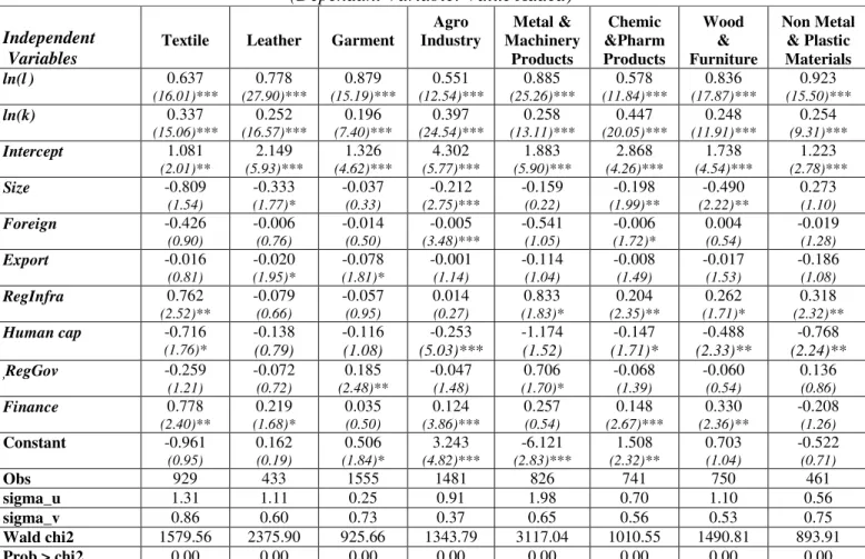
Results of estimation by industry are given in Table 7. Estimation results reinforce our previous findings. Production frontiers are robust to the introduction of different IC variables, with little changes in returns to scales or in the elasticities of production factors across industries. Countries specific conditions are also validated by the data.

One of the most interesting outcomes, nevertheless, concerns the investment climate which four dimensions are now significant with the expected sign34. Beside, our model

validates the impact of a much more substantial number of IC variables incorporated in the aggregated indicators. This result has to be stressed because it is the first time (to our knowledge) that the empirical literature brings evidences of the role of such a significant set of IC variables for such a large and diversified sample of industrial firms.

Table 7. Estimation Results: Common Model with Aggregated IC Variables

(Dependant Variable: Value Added)

Independent Variables

Textile Leather Garment

Agro Industry Metal & Machinery Products Chemic &Pharm Products Wood & Furniture Non Metal & Plastic Materials ln(l) 0.637 (16.01)*** 0.778 (27.90)*** 0.879 (15.19)*** 0.551 (12.54)*** 0.885 (25.26)*** 0.578 (11.84)*** 0.836 (17.87)*** 0.923 (15.50)*** ln(k) 0.337 (15.06)*** 0.252 (16.57)*** 0.196 (7.40)*** 0.397 (24.54)*** 0.258 (13.11)*** 0.447 (20.05)*** 0.248 (11.91)*** 0.254 (9.31)*** Intercept 1.081 (2.01)** 2.149 (5.93)*** 1.326 (4.62)*** 4.302 (5.77)*** 1.883 (5.90)*** 2.868 (4.26)*** 1.738 (4.54)*** 1.223 (2.78)*** Size -0.809 (1.54) -0.333 (1.77)* -0.037 (0.33) -0.212 (2.75)*** -0.159 (0.22) -0.198 (1.99)** -0.490 (2.22)** 0.273 (1.10) Foreign -0.426 (0.90) -0.006 (0.76) -0.014 (0.50) -0.005 (3.48)*** -0.541 (1.05) -0.006 (1.72)* 0.004 (0.54) -0.019 (1.28) Export -0.016 (0.81) -0.020 (1.95)* -0.078 (1.81)* -0.001 (1.14) -0.114 (1.04) -0.008 (1.49) -0.017 (1.53) -0.186 (1.08) RegInfra 0.762 (2.52)** -0.079 (0.66) -0.057 (0.95) 0.014 (0.27) 0.833 (1.83)* 0.204 (2.35)** 0.262 (1.71)* 0.318 (2.32)** Human cap -0.716 (1.76)* -0.138 (0.79) -0.116 (1.08) -0.253 (5.03)*** -1.174 (1.52) -0.147 (1.71)* -0.488 (2.33)** -0.768 (2.24)** ,RegGov -0.259 (1.21) -0.072 (0.72) 0.185 (2.48)** -0.047 (1.48) 0.706 (1.70)* -0.068 (1.39) -0.060 (0.54) 0.136 (0.86) Finance 0.778 (2.40)** 0.219 (1.68)* 0.035 (0.50) 0.124 (3.86)*** 0.257 (0.54) 0.148 (2.67)*** 0.330 (2.36)** -0.208 (1.26) Constant -0.961 (0.95) 0.162 (0.19) 0.506 (1.84)* 3.243 (4.82)*** -6.121 (2.83)*** 1.508 (2.32)** 0.703 (1.04) -0.522 (0.71) Obs 929 433 1555 1481 826 741 750 461 sigma_u 1.31 1.11 0.25 0.91 1.98 0.70 1.10 0.56 sigma_v 0.86 0.60 0.73 0.37 0.65 0.56 0.53 0.75 Wald chi2 1579.56 2375.90 925.66 1343.79 3117.04 1010.55 1490.81 893.91 Prob > chi2 0.00 0.00 0.00 0.00 0.00 0.00 0.00 0.00

Notes: The one step procedure explains firm-level inefficiency. The expected sign of the IC aggregated variables is positive for RegInfra, RegGovand Fin, and negative for H (see definition of variables in section 5). Variables Size, Foreign and

Export are also expected with a negative coefficient. All regressions contain country-dummy variables when estimating the production function. * significance level 10%; ** 5%; *** 1%. Absolute value of z statistics are in parentheses.

Source. Authors’ estimations

Findings by industry bring, as well, quite interesting comments. Human capital (Human), Infrastructure (Infra), and Financing Constraints (Finance) appear to be the most statistically significant investment climate factors for firm-level productivity. All three broad indicators explain quite well productivity discrepancies in most industries while Business-Government Relations (Gov) constitutes a less robust dimension. Our empirical analysis also reveals that some industries: Textile (for Human, Infra and Finance), Metal & Machinery Products (for Human and Gov) and Wood & Furniture (for Human and Finance) appear more sensitive and vulnerable than others in front of a deficit of their investment climate (the estimated coefficients of the IC variables are higher for these