HAL Id: hal-00371115
https://hal.archives-ouvertes.fr/hal-00371115v2
Submitted on 2 Nov 2009
HAL is a multi-disciplinary open access
archive for the deposit and dissemination of
sci-entific research documents, whether they are
pub-lished or not. The documents may come from
teaching and research institutions in France or
abroad, or from public or private research centers.
L’archive ouverte pluridisciplinaire HAL, est
destinée au dépôt et à la diffusion de documents
scientifiques de niveau recherche, publiés ou non,
émanant des établissements d’enseignement et de
recherche français ou étrangers, des laboratoires
publics ou privés.
MPLS label stacking on the line network
Jean-Claude Bermond, David Coudert, Joanna Moulierac, Stéphane Pérennes,
Hervé Rivano, Fernando Solano Donado
To cite this version:
Jean-Claude Bermond, David Coudert, Joanna Moulierac, Stéphane Pérennes, Hervé Rivano, et al..
MPLS label stacking on the line network. IFIP Networking, May 2009, Aachen, Germany. pp.809-820,
�10.1007/978-3-642-01399-7�. �hal-00371115v2�
MPLS label stacking on the line network
⋆ Jean-Claude Bermond1, David Coudert1, Joanna Moulierac1, StephanePerennes1, Herve Rivano1, Ignasi Sau1,2, and Fernando Solano Donado3
1
Joint project MASCOTTE, I3S(CNRS-UNS) INRIA, Sophia-Antipolis, France
2 Graph Theory and Combinatorics Group at Applied Mathematics IV Department
of UPC, Barcelona, Spain
3
Institute of Telecommunications, Warsaw University of Technology, Poland
Abstract. All-Optical Label Switching (AOLS) is a new technology
that performs forwarding without any Optical-Electrical-Optical conver-sions. The most promising scheme to manage the control plane of these optical networks is Generic MultiProtocol Label Switching (GMPLS). In this paper, we study the problem of routing a set of requests in GMPLS networks with the aim of minimizing the number of labels required to ensure the forwarding. In order to spare the label space, we consider label stacking, allowing the configuration of GMPLS tunnels. We study particularly this network design problem when the network is a line. We provide an exact algorithm for the case in which all the requests have a common source and present some approximation algorithms and heuris-tics when an arbitrary number of sources are distributed over the line. We analyze by simulations the performance of our proposed algorithms and compare them with previous ones.
1
Introduction
All-Optical Label Switching (AOLS) [2] is an approach to transparently route packets all-optically, allowing a speed-up of the forwarding. This very promising technology for the future Internet applications also brings new constraints and, consequently, new problems have to be addressed. Indeed, as the forwarding functions are implemented directly at the optical domain, a specific correlator is needed for each optical label processed in the node. Therefore, it is of ma-jor importance to reduce the number of employed correlators in every node, hence reducing the number of labels (as referred in the rest of the paper). The most promising scheme to manage the control plane of these optical networks is Generic MultiProtocol Label Switching (GMPLS). Therefore, for reducing the total number of labels in routers, solutions deployed by GMPLS for reducing the number of labels, such as label merging or label stacking, have to be studied.
In this paper we consider the problem of routing a set of given requests with the aim of minimizing the total number of labels. We study this problem when
⋆This work has been partly funded by the European project FET AEOLUS, the
COLOR INRIA LARECO and the project “Optimization Models for NGI Core Network” (Polish Ministry of Science and Higher Education, grant N517 397334).
the network is a line and when label stacking allowing to configure GMPLS tunnels is considered. Restricting the problem to the case when the network is a line will provide efficient algorithms that are necessary to better apprehend the general problem.
The first studies related to label space reduction in GMPLS networks are based on a technique called label merging (not discussed here). Saito et al. were the first considering this problem and they propose in [3] a linear programming mathematical model to find the most efficient routing solution in terms of labels using label merging. It is worth mentioning the heuristic proposed by Bhatnagar et al. in [1] with the same aim. The contributions using label merging were further extended in [7].
In [8] the authors deal with the problem of minimizing the number of used labels, when routes are given and the stack depth is limited to two. In [4], the authors extend this problem by assuming that routes should be found as well, considering that links have capacities. In these two contributions, the authors have as objective the minimization of the usage of the label space while keeping the stack depth to a maximum of two, which can be seen as a network design problem since the goal is to find the minimum capacities in the nodes to satisfy a traffic matrix.
This paper is organized as follows. In Section 2, we recall the basic concepts of GMPLS label forwarding mechanism. In Section 3, we formally state the problem addressed in this paper. In Section 4, we present a optimal polynomial-time algorithm when one source is considered in the line. In Section 5, we propose an approximation algorithm and heuristics when multiple sources are considered. Simulation results concerning these algorithms are reported in Section 6. Finally, Section 7 gives conclusion and perspectives of the work.
2
Label Switching Mechanism in GMPLS
In GMPLS, requests are established by the configuration of Label Switched Paths (LSPs). Packets are associated to LSPs by means of a label, or tag, placed in the header of the packet. In this way, routers - called Label Switched Routers (LSR) - can distinguish and forward packets. In addition, in GMPLS, it is allowed to carry a set of labels in packets header, conforming a stack of labels. Even though a packet may contain more than one label, LSRs must only read the first (or top) label in the stack in order to take forwarding decisions. Stacking labels and label processing, in general, is standardized by the following set of operations that an LSR can perform over a given stack of labels:
– SWAP: replace the label at the top by a new one,
– PUSH: replace the label at the top by a new one and then push one or more onto the stack, and
– POP: remove the label at top in the label stack.
The labels stored in the forwarding table are significant only locally at the node and swapped all along the LSP.
λ κ ι λ l:l SWAP l1,out:BC l2: POP,out:DE l1:l1 SWAP l2,out:CD units of traffic λ k1:PUSH l,out:AB k :PUSH l,out:AB k :PUSH l,out:AB k :PUSH l,out:AB k2:PUSH l,out:AB PUSH ... ... E D C B A Data Payload l ki ki Data Payload Data Payload Data Payload Data Payload Data Payload Data Payload kλ kκ kι k 2 k1
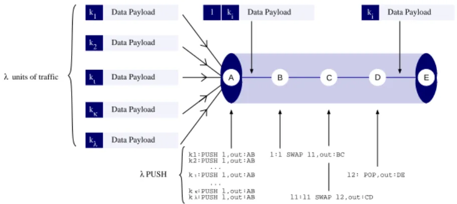
Fig. 1.GMPLS Operations performed at the entrance and at the exit of a tunnel.
Label stacking
When two or more LSPs follow the same set of links, they can be routed together ‘inside’ a higher-level LSP, henceforth a tunnel. In order to setup a tunnel, mul-tiple labels are placed in the packet’s header: a method known in the literature as label stacking.
As mentioned before, the LSRs in the core of the network route data solely on the basis of the topmost label in the stack. This helps to reduce both the number of labels that need to be maintained on the core LSRs and the complexity of managing data forwarding across the backbone.
Figure 1 represents the general operations needed to configure a tunnel with the use of label stacking. At the entrance of the tunnel, λ PUSH are performed in order to route the λ units of traffic through the tunnel. Then, only type one operation (either a SWAP or a POP at the end of the tunnel) is performed in all the nodes along the tunnel, regardless of λ. In this figure, a stack of size 2 is used to route the λ LSPs in one tunnel from node A to node E. The top label l is swapped and replaced at each hop: by l1 at node B, by l2 at node C, and
is finally popped at node D. The λ units of traffic, at the exit of the tunnel at node E can end or follow different paths according to their bottom label ki, for
all i ∈ {1, 2, ..., w} in the stack.
Therefore, the total cost c(T ) of this tunnel T = (A, E) in terms of number of labels is: c(T ) = λ + l(T ) − 1, where λ is the number of units of traffic forwarded through this tunnel and l(T ) is its length in terms of number of hops (which is 4 on this example).
The traffic can enter in any node of a tunnel but can exit in only one point, the last node of the tunnel. In other words, when some traffic is carried by a tunnel, it follows the tunnel until the end.
This cost function c(T ) still holds for some degenerated cases. For example, in the case of an arc (i.e., a path of length 1, l(T ) = 1), or when one unit of traffic is routed in a path (i.e., a single LSP with λ = 1 whose cost is only its length). In the following, we consider as a tunnel, without loss of generality: (1)
an arc routing several units of traffic, (2) a path routing a only one unit of traffic, and (3) a path routing several units of traffic (i.e., λ > 1 and l(t) > 1). Note that strictly speaking, only the third case is considered as a tunnel.
In this paper, we fix the maximum stack size to 2. Increasing the stack size, increases also the total bandwidth consumption in the network. When the size of the stack is not limited, label stripping [9, 10] encoding the whole path in the stack provides a feasible solution.
3
Modelling the LSPR problem
This section describes the problem of routing a set of requests in GMPLS network with the aim of minimizing the number of labels. The problem is formally defined as follows:
Label Space Reduction in a GMPLS Network: LSPR
Input:a network (digraph) G = (V, E) and a set of requests R, where in the request r ∈ R, r = (si, uj), si∈ V sends wr units of traffic to uj ∈ V .
Output:A set T of tunnels enabling to route the traffic and a dipath composed of tunnels in T for each request (si, uj).
Objective: minimize the total cost of T , that is c(T ) =PT
k∈T c(Tk) where
the cost c(Tk) of a tunnel Tkwhich contains λkunits of traffic and is of length
l(Tk) (number of arcs in G associated to the path joining the end-vertices of
Tk) is c(Tk) = λk+ l(Tk) − 1.
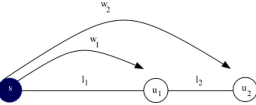
Computation of a solution to the example of Figure 2. Consider the line network with one source s, w1 units of traffic destined to u1at distance l1from s (l1− 1
nodes between s and u1) and w2units of traffic destined to u2 at distance l1+ l2
from s. See Figure 2 for an illustration. The optimal solution depends on the values li and wi. Indeed, two solutions have to be examined.
In the first solution, a specific tunnel (s, ui) is configured for each destination
ui, giving two tunnels (s, u1) and (s, u2) with a total cost: (w1+ l1− 1) + (w2+
l1+ l2− 1) = w1+ w2+ 2l1+ l2− 2.
The second solution is composed of the two tunnels (s, u1) and (u1, u2). The
requests destined to u2 will first use the tunnel (s, u1) and then the tunnel
(u1, u2). The traffic carried by (s, u1) is λ1= w1+ w2 and the traffic carried by
(u1, u2) is λ2= w2. Therefore, the total cost is (w1+w2+l1−1) + (w2+l2−1) =
w1+ 2w2+ l1+ l2− 2.
The optimal solution is either the first one if l1 ≤ w2 or the second one if
l1≥ w2.
Lemma 1 In any network G = (V, E), there exists an optimal solution T for the problem LSPR such that all the units of traffic of the request (si, uj) are
routed in T via a unique dipath (set of consecutive tunnels) from si to uj.
Proof. Let T be an optimal solution and suppose that the requests arriving at ujare routed via p > 1 different paths P1, . . . , Pm. Let λm, 1 ≤ m ≤ p, be the
w l l w u s 1 1 1 2 u2 2
Fig. 2. Depending on the values l1 and w2, the optimal solution may be composed
either of tunnels (s, u1) and (s, u2), or of tunnels (s, u1) and (u1, u2).
number of traffic units forwarded by Pm. Let hm (h like hops), 1 ≤ m ≤ p, be
the number of consecutive tunnels in the path Pm. Let the order of the paths be
such that P1 is a path with the minimum number of consecutive tunnels h1.
Then, for any other path Pm(m > 1) reroute the λmrequests routed via Pm
via P1. We obtain a new feasible solution T′ whose cost is
c(T′) ≤ c(T ) + λmh1− λmhm.
Indeed, the cost of each tunnel used in Pmis decreased by λm, plus possibly,
if some tunnel T of Pmbecomes empty, by l(T ) − 1 ≥ 0. On the other hand, the
cost of each tunnel of P1 is increased only by λm as the tunnel already exists.
Therefore, as h1 ≤ hm, we get c(T′) ≤ c(T ) with strict inequality if h1 < hm
(the path Pmis strictly longer than P1) or if, in the rerouting, some tunnels of
length more than 1 become empty. So T′ is also an optimal solution.
Repeating the operation for each Pmwe obtain an optimal solution T∗, where
all the requests arriving at a node ui are routed in T via a unique dipath. ⊓⊔
The cost of an optimal solution T for problem LSPR with |T | tunnels and |R| requests is: c(T ) = |T | X k=1 (l(Tk) − 1) + |R| X r=1 hrwr.
where hr is the number of consecutive tunnels for the request r in T , wr
is the number of units of traffic of the request r and l(Tk) is the length of the
tunnel Tk in terms of number of hops. The cost c(T ) is the sum of the cost for
the configuration of the tunnels (P|T |k=1(l(Tk) − 1)) and the cost for the requests
to enter the tunnels (P|R|r=1hrwr).
4
LSPR-L1 problem: the line network, one source
In this section, we focus on the specific case when the network G = (V, E) is a directed line (a dipath) and when the number of sources is equal to 1. Focusing on the same problem with simplest constraints will provide algorithms that will be useful to find efficient solutions for the general problem. Let us denote by Ps→un
s uj uα ul
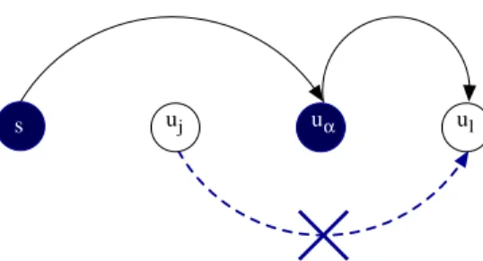
Fig. 3.The tunnel in dotted points is not present in an optimal solution.
indexed in the increasing order of their distance from s. This problem is referred as LSPR-L1 in the sequel (standing for Label Space reduction in a GMPLS Line Network with 1 source). The main result of this section is an algorithm based on dynamic programming techniques that finds an optimal solution in time O(n3),
as stated in Proposition 1. First, we need two technical lemmas.
Lemma 2 When the network is a directed line, with source s, an optimal solu-tion T for LSPR-L1 problem is such that, if (s, uα) is the longest tunnel from
s, then there is no tunnel (uj, ul) in T with j < α < l.
Proof. Suppose there exists such a tunnel (uj, ul) (see Figure 3). As α is the
maximum index, then uj 6= s, otherwise (s, ul) would have been longer than
(s, uα). Therefore, the number of consecutive tunnels towards ul, h(s,ul)denoted
simply hl, satisfies: hl≥ 2. Consider the solution T′obtained from T by deleting
the tunnel (uj, ul) and adding, if it does not exist, the tunnel (uα, ul). The request
(s, ul) is then routed through two consecutive tunnels (s, uα) and (uα, ul). It is
an admissible solution whose cost satisfies:
c(T′) ≤ c(T ) − λlhl− (l(uj, ul) − 1) + 2λl+ l(uα, ul) − 1,
where λl is the number of requests arriving at ul. As hl ≥ 2 and l(uα, ul) <
l(uj, ul), c(T′) < c(T ). ⊓⊔
Lemma 3 For a line Ps→un with wi units of traffic for the request (s, ui), the
cost of an optimal solution is:
c∗(Ps→un) = min α [ n X i=α wi+ l(s, uα) − 1 + c∗(Ps→uα−1) + c ∗(P uα→un) ],
where uα∈ Pu1→un is a splitting point that decomposes the problem into two
sub-problems.
Proof. By Lemma 2 an optimal solution contains a tunnel (s, uα) of cost (
Pn i=αwi+
l(s, uα) − 1) plus an optimal solution on the sub-line Ps→uα−1 and an optimal
Algorithm 1: Polynomial-time algorithm computing an optimal solution for the LSPR-L1 problem.
Input: Line Ps→un from s to un, where s is the source (referred also as u0)
and (s, ui) are the set of requests (i ≥ 1), each of them having wiunits
of traffic
Output: Set of tunnels enabling the routing from s of all the requests (s, ui)
begin
Cis a table of size n2 indicating the costs all the sub-solutions;
S is a table of size n2
indicating the splitting points uα associated to the
optimal sub-solutions;
W is a table of size n storing partial sums of weigths, W [0] = 0, W [j] =
Pj i=1wi= W [j − 1] + wj, and so Pβ i=αwi= W [β] − W [α − 1]; fori ∈[0, n] do C[ui, ui] = 0;
C[ui, ui+1] = wi+1+ l(ui, ui+1) − 1;
S[ui, ui+1] = ui+1;
fori ∈[2, n] do
for ∀k ∈[0, n − i] do
min= +∞;
for ∀α ∈[k + 1, k + i] do
value= (W [k + i] − W [α − 1]) + l(uk, uα) − 1 + C[uk, uα−1] +
C[uα, uk+i];
if value < min then
min= value;
C[uk, uk+i] = c(Puk→uk+i) = value; S[uk, uk+i] = uα;
Compute the optimal set of tunnels from the table S; end
Proposition 1 When the network is a directed line Ps→un, and all requests
are issued from s, then an optimal solution of the LSPR-L1 problem can be computed in time O(n3) by Algorithm 1.
Proof. According to Lemma 3, to compute an optimal solution for Ps→un, we
need first to compute optimal sub-solutions for Ps→uα−1 and for Puα→un, uα∈
{u1, . . . , un}, and recursively. The algorithm computes first solutions for Pui→ui+1,
and for computing solutions for Pui→ui+2, the already computed values for
sub-lines Pui→ui+1(say C[ui, ui+1]) and Pui+1→ui+2(say C[ui+1, ui+2]) are used
with-out any recomputation.
For example, to compute the solution on Ps→u2, we need the values C[s, u1]
and C[u1, u2] since we have C[s, u2] = min{(w1+ w2+ l(s, u1) − 1 + C[u1, u2]),
(w2+l(s, u2)−1+C[s, u1])}. Now, if we want to compute the solution on Ps→u3,
we need to compute first C[u1, u3] and C[u2, u3], but not C[s, u1] and C[s, u2]
(s,u1) (u1,u2) (s,u3) (u3,u4) w = 20 w = 10 w = 10 w = 10 11 11 11 11 3 4 2 1 u1 u2 u3 u4 s
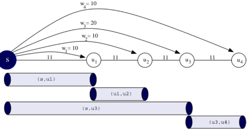
Fig. 4.An example with its optimal solution.
Finally, we can compute the optimal solution using dynamic programming (Algorithm 1), with time complexity O(n3) and space complexity O(n2). ⊓⊔
The optimal algorithm in the example of Figure 4. Let us compute an optimal solution to the example in Figure 4 using Algorithm 1. We first have to compute the table C containing the costs of the sub-optimal solutions for each sub-line.
First, the sub-paths of length 1, Ps→u1, Pu1→u2, Pu2→u3, and Pu3→u4 are
straightforward computed in C[u0, u1], C[u1, u2], C[u2, u3], and C[u3, u4].
Then, for the sub-paths of length 2, Ps→u2, Pu1→u3, and Pu2→u4, two splitting
points are considered by the algorithm. For example, for Ps→u2, the optimal
solution implies a splitting point u1with cost w1+ w2+ l(s, u1) − 1 + C[u0, u0] +
C[u1, u2] = 50 (the splitting point u2 implying a greater cost w2+ l(s, u2) − 1 +
C[u0, u1] + C[u2, u2] = 51). The already computed costs C[u0, u0], C[u1, u2], and
C[u2, u2] have been used by the algorithm and are not computed again.
For the computation of the optimal solution on the whole line Ps→u4, four
splitting points, u1, u2, u3, and u4 should be considered.
When the table C showing the optimal costs for all the subpaths has been computed as presented in Table 1, the set of tunnels composing the optimal solution can be deduced from the splitting points. The optimal solution for line Ps→u4 has cost 132 and a splitting point u3. Thus, the optimal solution is
composed of a tunnel (s, u3) and of optimal solutions for the sub-paths Ps→u2
and Pu3→u4. The first sub-solution has a splitting point u1 which gives tunnels
(s, u1), (u1, u2). The optimal solution for the sub-path Pu3→u4 is obviously the
tunnel (u3, u4).
Finally, the optimal solution is composed of tunnels (s, u1), (u1, u2), (s, u3),
and (u3, u4).
In the special case where the requests are uniform, we are able to give a closed formula of the cost of an optimal solution, as stated as follows.
s= u0u1 u2 u3 u4 s= u0 0 20 50 (u1) 101 (u2) 132 (u3) u1 - 0 20 61 (u3) 91 (u3) u2 - - 0 30 60 (u3) u3 - - - 0 20 u4 - - - - 0
Table 1.Computation of the table C and S for the optimal solution of the example
on Figure 4, the nodes in brackets representing the splitting points of table S.
Proposition 2 For a line network Ps→un, with n = 2
q − 1 + r, where 0 ≤ r ≤
2q− 1, and an uniform distribution: ∀i, w
i= 1, the cost of an optimal solution
is 2q(q − 1) + 1 + (q + 1)r.
The proof of this proposition is technical and is not given in this paper due to lack of space. In this specific case we can prove that c∗(P
s→un) = c ∗(P
s→un−1) +
⌊log(n)⌋ + 1.
5
LSPR-LM problem: the line network, multiple sources
In this section, we study the problem of routing a set of requests on the line network when multiple sources are distributed along the line. Since sources may inject traffic anywhere in the network, Lemma 2 is not valid anymore, hence the problem seems to be inherently more complicated. As the problem cannot be decomposed as easily as previously, we present in this section a log(n)−approximation algorithm and an heuristic that will be compared to the optimal solution and to previous known heuristics in Section 6. The problem is referred in the following as LSPR-LM (standing for Label Space reduction in a GMPLS Line Network with Multiple sources).
5.1 log(n)-approximation algorithm for LSPR-LM
Consider the nodes {u0, u1, . . . , un}, that can be source or destination or both,
sorted according to their position on the line from the left to the right (ui+1
after ui on the line, ui+1 being at distance li+1 from ui). Suppose that the line
is of length L, meaning that L =Pni=1li.
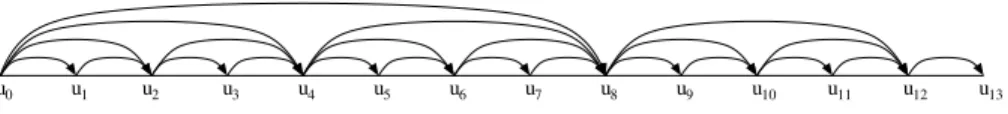
The algorithm consists of configuring all the consecutive tunnels {(u0, u1),
(u1, u2), . . . , (un−1, un)}, {(u0, u2),(u2, u4), . . . ,(un−2, un)}, {(u0, u4), (u4, u8),
. . . ,(un−4, un)}, and more generally, those of length a power of 2. See Figure 5
for an illustration of the configuration of the tunnels. Consequently, there exists a path of at most log(n) tunnels from any source to any destination, ensuring a valid routing for all the requests. When the solution has been computed, then some tunnels that are not used by any destination may be removed.
Theorem 1 For a problem with n sources and/or destinations, there exists a log(n)-approximation algorithm for the LSPR-LM problem.
u u u u u u
u0 1 2 3 4 5 6 u7 u8 u9 u10 u11 u12 u13
Fig. 5. Computing this set of tunnels gives a log(n)−approximation algorithm for
LSPR-LMproblem.
Proof. The cost of a solution computed by the algorithm is (1) the cost of the configuration of the tunnels plus (2) the cost for entering the tunnels.
To configure each level of consecutive tunnels, at most L−1 labels are needed. There are at most log(n) different levels of tunnels. So, the overall number of labels needed for the configuration of tunnels is at most (1) ≤ (L − 1) log(n).
When that set of tunnels has been configured, any source can join any des-tination in at most log(n) hops. Therefore, the total cost needed to enter the tunnels is at most (2) ≤P|R|r=1wrlog(n).
Then, the cost of this solution is at most: (1) + (2) ≤P|R|r=1wrlog(n) + (L −
1) log(n) = log(n)(P|R|r=1wr+ L − 1).
In the best case, an optimal solution will be of costP|R|r=1wr+ (L − 1), giving
a log(n)−approximation. ⊓⊔
5.2 Proposed heuristic: Extended Dynamic Programming
This subsection presents a simple heuristic to find a solution of the problem on the line with multiple sources. Suppose that, when constructing the solution, there is a set of tunnels leading from a source u0 to a destination ui. Then, if
another source, say ux with x > 1, has to transmit traffic to ui, then ux may
insert traffic directly in the tunnels going to ui without additional cost.
Therefore, the heuristic consists of considering only the source u0, then, to
affect the whole set of requests to u0 and to use the polynomial algorithm just
described previously for only one source. In the solution, there would be tunnels from u0 to all the destinations, and the other sources will insert their traffic in
the tunnels passing through them.
6
Simulations
In this section we analyze the performance of the proposed heuristics using simulations. The analysis consists of the comparison of the total number of labels used by the heuristics.
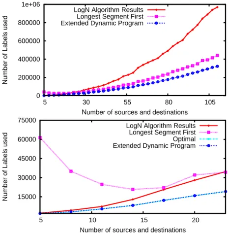
In our simulations, we use a line network consisting of 500 nodes. Each ex-periment consists of a different number of sources and destinations. The number of sources equals the number of destinations in each experiment. Between a pair of source and destination nodes, a demand is generated (with a probability of 80%) with a random capacity between one and 500 (uniform).
0 200000 400000 600000 800000 1e+06 5 30 55 80 105
Number of Labels used
Number of sources and destinations LogN Algorithm Results
Longest Segment First Extended Dynamic Program
15000 30000 45000 60000 75000 5 10 15 20
Number of Labels used
Number of sources and destinations LogN Algorithm Results
Longest Segment First Optimal Extended Dynamic Program
Fig. 6.Comparison on the number of labels used by different heuristics and
magnifi-cation of the first 20 experiments including the optimal solution.
Figure 6 (top) shows the behavior the heuristics proposed in this article together with the Longest Segment First (LSF) heuristic [5]. The number of sources (or destinations) varies from 5 to 113 with increments of three nodes in each experiment. Each experiment was run 100 times. The results show that, even though the log(n)-approximation runs in O(p log n) and guarantees a bound in terms of sub-optimality, in practice the results are not as good as the proposed Extended Dynamic Programming heuristic or the LSF heuristic running in O(n3)
and O(np2), respectively. We also observed that the requirements in memory for
LSF are lower than those of the Extended Dynamic Programming heuristic; however the quality of the solution of the later always outperforms the former’s. Some other previously proposed heuristics (see [4] and [6]) were tested as well with worse results, hence not considered in this analysis.
At the bottom of Figure 6, a magnification of the results in the first 20 experiments is shown. The plot showing the optimal value is also added. In
these experiments, the numerical solution computed by the heuristic based in dynamic programming is within 1% (in most of the case) of the optimal value. We conjecture that this is because the demands share the same set of destinations. The proposed heuristics in this paper show a better convergence than that of LSF when the number of sources is low.
7
Conclusion and perspectives
We presented in this paper the problem of routing a set of requests with the aim of reducing the total number of labels in the network. For the line, we exhibit a polynomial-time algorithm when there is a single source and a log(n)-approximation algorithm, and one heuristic for multiple sources. We show the good performance of these algorithms through simulations. In future work, we plan to extend these proposed algorithms to general networks and to study the computational complexity of the LSPR problem.
References
1. S. Bhatnagar, S. Ganguly, and B. Nath. Creating Multipoint-to-Point LSPs for traffic engineering. IEEE Commun. Mag., 43(1):95–100, Jan. 2005.
2. F. Ramos et al. IST-LASAGNE: Towards all-optical label swapping employing optical logic gates and optical flip-flops. IEEE J. Sel. Areas Commun., 23(10):2993– 3011, Oct. 2005.
3. H. Saito, Y. Miyao, and M. Yoshida. Traffic engineering using multiple
MultiPoint-to-Point LSPs. In IEEE Conference on Computer Communications (Infocom
2000), pages 894–901, 2000.
4. F. Solano, R. V. Caenegem, D. Colle, J. L. Marzo, M. Pickavet, R. Fabregat, and P. Demeester. All-optical label stacking: Easing the trade-offs between routing and architecture cost in all-optical packet switching. In IEEE Conference on Computer Communications (Infocom 2008), pages 655–663, Phoenix, AZ, USA, Apr. 2008. 5. F. Solano, R. Fabregat, Y. Donoso, and J. Marzo. Asymmetric tunnels in P2MP
LSPs as a label space reduction method. In Proc. IEEE International Conference on Communications (ICC 2005), pages 43–47, May 2005.
6. F. Solano, R. Fabregat, and J. Marzo. A fast algorithm based on the MPLS label stack for the label space reduction problem. In Proc. IEEE IP Operations and Management (IPOM 2005), Oct. 2005.
7. F. Solano, R. Fabregat, and J. Marzo. On optimal computation of MPLS label binding for MultiPoint-to-Point connections. IEEE Trans. Commun., 56(7):1056– 1059, July 2007.
8. F. Solano, T. Stidsen, R. Fabregat, and J. Marzo. Label space reduction in MPLS networks: How much can a single label do? IEEE/ACM Trans. Netw., Dec. 2008. 9. R. Van Caenegem et al. Benefits of label stripping compared to label swapping from the point of node dimensioning. Photonic Network Communications Journal, 12(3):227–244, Dec. 2006.
10. R. Van Caenegem et al. From IP over WDM to all-optical packet switching: Economical overview. J. Lightw. Technol., 24(4):1638–1645, Apr. 2006.