Correlation of NSWC grounding tests with MIT theory

(1)

CORRELATION OF NSWC GROUNDING TESTS

WITH MIT THEORY

by

Ifiigo Javier Puente

B.S. Ocean Engineering

Massachusetts Institute of Technology (1994)

Submitted to the Department of Ocean Engineering in Partial Fulfillment of the Requirements

for the Degree of

MASTER OF SCIENCE In Ocean Engineering

at the

MASSACHUSETTS INSTITUTE OF TECHNOLOGY May 1995

The author hereby grants to MIT permission to reproduce and to distribute publicly paper and electronic copies of this thesis document in whole or in part.

/ Signature of Autho..

'T/2

A

Department of Ocean EngineeringMay 1995 Certified by

Tomasz Wierzbicki, Professor of Applied Mechanics Thesis Supervisor

i -

,-Accepted by.

A. Douglas Carmichael, Chairman Deartment Gfaduate Committee Department of Ocean Engineering

;MASSACUSrETTS INSti'UiE

OF TECHNOLOGY f

d w

(2)

-CORRELATION OF NSWC GROUNDING TESTS

WITH MIT THEORY

by

Ifiigo Javier Puente

Submitted to the Department of Ocean Engineering on May 17, 1995, in partial fulfillment of the requirements for the degree to Master of Science in Ocean Engineering.

ABSTRACT

Over the last three years, the Joint MIT-Industry Program on Tanker Safety has conducted extensive research on the subject of ship grounding and collision accidents. In a previous Tanker Safety Report [2], the NSWC large scale grounding experimental results were used to validate the existing Minorsky/Vaughn theory. The correlation was shown to leave room for improvement. In this thesis, a complete new theoretical approach to the problem of ship grounding is developed. This new approach is based on the concept of Superelements that was first introduced in the automotive industry. The underlying principle of the new theory is to investigate the separate contributions of the large structural elements identified in the model, and then to assemble those contributions into the total response of the structure. In this thesis, it will be shown that the correlation of the new MIT theory with NSWC large scale grounding experimental results constitutes a significant improvement on the existing Minorsky/Vaughn theory.

Thesis Supervisor: Tomasz Wierzbicki Title: Professor of Applied Mechanics

(3)

Acknowledgment

First and foremost, I would like to thank my advisor Professor Tomasz Wierzbicki for his guidance and help in completing this thesis. I would also like to thank the research team of the Joint MIT-Industry Program on Tanker Safety, including Dr. Sung K. Choi of Deawoo, Dan Pippenger of MIT, and Bo Simonsen of the Technical University of

Denmark, for their contributions to the development of the new ship grounding theory. Many thanks are due to Teresa Coates for her invaluable help in dealing with administrative matters.

I wish to extend my gratitude to all the people that over my five years at MIT have impressed upon me the desire of learning which has culminated in this masters thesis.

Finally, I would like to offer a special recognition for my mother Agurtzane, my family, and my friends, for their love and support, without which any enterprise would lose its meaning. To them I dedicate this thesis.

(4)

Force...

(53)

4.3.2 Geometry of Inner Plate Steady State Cutting ... (54)

4.3.3 Inner Plate Steady State Cutting Boundaries ... (54)

4.4 Summary of Inner Plate Contribution to the Total Resisting Force ... (54)

Chapter 5. Contribution of Transverse Frames to the Total Resisting Force ... (61)

5.2 Transverse Frame Cutting Force Governing Equation ... (62)

5.3 Transverse Frame Contribution Boundaries ... (63)

5.4 Summary of Transverse Frame Contribution to the Total Resisting Force ... (64)

Chapter 6. Contribution of Longitudinal Girders to the Total Resisting Force ... (70)

(6)

6.2.1 Model Kinematics ... (70)

6.2.2 Energy Dissipation . ... (71)

6.2.3 Friction Contribution to the Longitudinal Girder Crushing Force ...(72)

6.2.4 Closed Form Solution for the Longitudinal Girder Crushing Force ...(72)

6.3 Longitudinal Girder Contribution Boundaries ... (73)

6.4 Summary of Longitudinal Girder Contribution to the Total Resisting Force ...(74)

Chapter 7. Conclusion ... (79)

7.1 Comparison of MIT Theory with NSWC Grounding Test ... (79)

7.2 Recommendations for Future Work ... (81)

7.3 Final Remarks ... (82)

References

...

(84)

Appendix

...

(86)

Al. Table of Numerical Values ... (77)

A2. Matlab Source Code ... (77)

(7)

List of Figures

Figure 2.1. Schematic View of NSWC Experimental Apparatus ...(18)

Figure 2.2. NSWC Grounding Test T-5 Model Geometry ...(19)

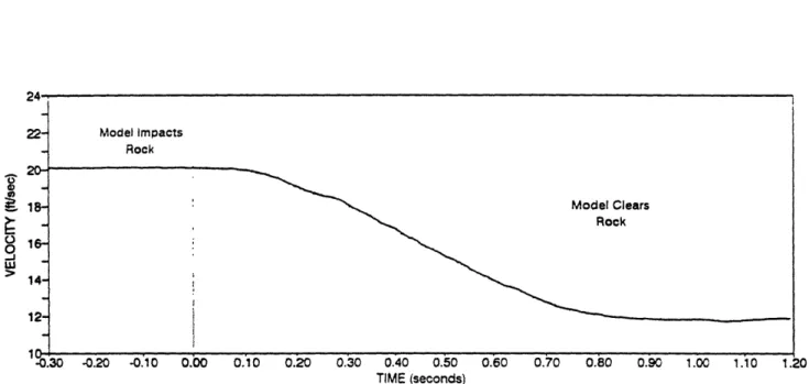
Figure 2.3. NSWC Grounding Test Velocity Data ...(20)

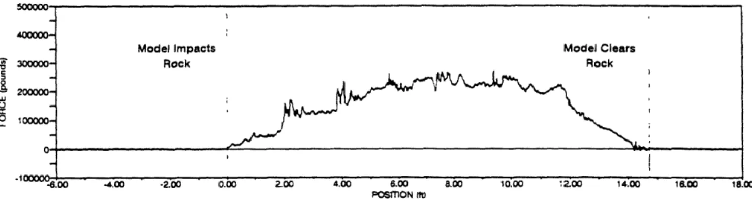
Figure 2.4. NSWC Grounding Test Rock Reaction Forces ... (21)

Figure 2.5. Global Coordinate System for Hull-Cone Interaction ...(22)

Figure 3.1. Aerial View of Cone Cutting through Outer Plate ...(40)

Figure 3.2. Outer Plate Initiation Force vs. Split Angle ...(41)

Figure 3.3. Curved Flaps Model Geometry ... (42)

Figure 3.4. Local Coordinate System for Curved Flaps Model ...(43)

Figure 3.5. Side View of Cone-Outer Plate Interaction . ... (44)

Figure 3.6. Outer Plate Steady State Force vs. Split Angle ...(45)

Figure 3.7. Theoretical Contribution of Outer Plate to the Total Resisting Force ...(46)

Figure 4.1. Inner Plate Cutting Initiation Geometry ...(56)

Figure 4.2. Straight Flaps Model Geometry ... (57)

Figure 4.3. Side View of Cone-Inner Plate Interaction ...(58)

Figure 4.4. Inner Plate Steady State Force vs. Split Angle ... (59)

Figure 4.5. Theoretical Inner Plate Contribution to the Total Resisting Force ...(60)

Figure 5.1. Transverse Frame Geometry ... (66)

Figure 5.2. Diamond Shape Geometry in Transverse Frame Cutting ...(67)

Figure 5.3. Phases of Transverse Frame Cutting ... (68)

Figure 5.4. Theoretical Transverse Frame Contribution to the Total Resisting Force ...(69)

Figure 6.1. Longitudinal Girder Deformation Geometry ...(75)

Figure 6.2. Side View of Longitudinal Girder Deformation Geometry ...(76)

Figure 6.3. Longitudinal Girder Force vs. Split Angle ... (77)

Figure 6.4 Theoretical Longitudinal Girder Contribution to the Total Resisting Force ...(78)

(8)

List of Tables

Table 2.1. Summary of NSWC Experiment Global Parameters ...(15)

Table 3.1. Summary of Outer Plate Contribution to the Total Resisting Force ...(39)

Table 4.1. Summary of Inner Plate Contribution to the Total Resisting Force ...(55)

Table 5.1. Summary of Transverse Frame Contribution to the Total Resisting Force ...(65)

Table 6.1. Summary of Longitudinal Girder Contribution to the Total Resisting Force...(73)

(9)

List of Symbols

0 Plate split angle.

q~ Cone apex angle measured from the vertical. ao Material flow stress.

t Plate thickness for all structural members. It Coefficient of friction.

a Angle of attack of structural assembly with respect to the ground. cl Transverse frame spacing.

c2 Perpendicular distance from outer plate leading edge to the first transverse frame. R Stable flap rolling radius.

V Forward horizontal velocity of the structure with respect to the cone.

B Curved flap induced conical wedge shoulder.

h Vertical distance from cone vertex to the undeformed outer plate. A Height of the 90 degree cone.

A1 Height of the conical rock.

r Radius of the conical rock rounded tip dome.

1 Overall length of model assembly.

[~ Rotation of the straight flap with respect to the undeformed inner plate. 56 Vertical penetration of the conical rock into the inner plate.

d Double hull height.

e Perpendicular distance between top of spherical rock and outer plate leading edge.

x,y Global coordinate system. , 7/ Local coordinate system.

(10)

Chapter 1 Introduction

1.1 Introduction

Over the last two years three large-scale oil tanker grounding experiments have been conducted by the Carderock Division of the Naval Surface Warfare Center (NSWC). An additional eight tests are being planned in the near future. At the time of this writing only results from the first grounding experiment were published in the open literature, Rodd [1]. This experiment represents a typical section of a conventional double hull tanker bottom structure with longitudinal and transverse framing. The T-5 Panel Buck geometry and scantlings were used for the one-fifth scale Grounding Model #1. The Grounding Model #1 is considered to be the baseline for subsequent, more elaborated double hull

structural designs, and, therefore, the most general and representative case.

The objective of this thesis is to predict the total resisting force of the structure in the event of grounding against a conical rock and compare it with NSWC test results. In an earlier effort by Choi et al. [2], the grounding force developed in NSWC Model #1 was determined using the MinorskyNaughn method. The validity, in large scale experiments, of the Minorsky/Vaughan empirical formula, [13], [14], [15] and [16], for the prediction

of the energy absorbed by a ship hull structure during collision and grounding accidents, has been challenged by Choi's correlation between the Minorsky approach and the NSWC Grounding Tests results, Choi et al. [2]. Choi found that this correlation was not satisfactory, both in terms of the magnitude of the grounding force and the total energy dissipated. The deficiencies in the Minorsky/Vaughan method can be attributed to three factors:

(11)

1. The inherent difficulty of defining the amount of damaged material around the rock, or other underwater obstacles.

2. The independence of Minorsky's empirical formula on the magnitude of the material yield stress, and hence its inability to distinguish amongst different types of materials, e.g. mild steel versus high strength steel.

3. The difficulty of determining the displaced volume of ship hull material and the area of tearing fracture for complex ship hull geometry, such as in the case of NSWC Grounding Tests.

In the present report, an alternative method of predicting grounding forces is introduced, based on the concepts of Superfolding and Supertearing elements. The Superelement approach to grounding calculations was developed for the Joint MIT-Industry Program on Tanker Safety and is documented in a number of technical reports. Each of these reports addressed particular failure modes of single structural elements. Examples of failure modes considered so far are concertina tearing of hull plating [9], central separation (also known as clean cut) [4], crushing of webs [10] and [11], and cutting of transverse frames and bulkheads [121. Good correlation with small, intermediate and full scale tests was obtained at the level of individual structural elements.

A section of a double hull tanker represents a complex structural system. The NSWC intermediate scale test provides a perfect opportunity to validate the MIT theory in a realistic grounding configuration. However, the conical rock geometry and the relative position of the rock with respect to the double hull used in the NSWC test have introduced a number of failure modes that had not been considered in the existing reports of the Tanker Safety Program. In an attempt to improve the analytical techniques for predicting damage to ships in collision and grounding accidents, the Joint MIT-Industry Program on Tanker Safety was commissioned by NSWC to conduct additional research and develop new theoretical models for the prediction of damage. The correlation of the new MIT theory with NSWC Grounding Tests results has turned out to be an improvement over the existing Minorsky/Vaughan method.

(12)

The spirit of the MIT theory is to investigate the individual contributions of all structural members present in the double hull ship structural configuration of NSWC Grounding Tests, and to account for the effect of the material yield stress in all calculations.

In this document, theoretical models are developed for the energy dissipation modes of each contributing structural member and, in the end, the individual contributions are assembled and compared with the results of the NSWC Grounding Tests.

All calculations were conducted using Matlab software. A hard copy of the input file is included in the Appendix.

(13)

Chapter 2 Description of NSWC Grounding

Experiment

2.1 Description of the Experimental Apparatus

In NSWC tests, the Grounding Test Machine developed by HI-TEST Laboratories, Inc., in Arvonia, Virginia, is employed. The Grounding Test Machine enables researchers to simulate grounding conditions for Oil Tanker in the 30,000 to 40,000 ton category, at one-fifth scale. Figure 2.1 shows a schematic view of the experimental apparatus.

The test vehicle, weighing 223 tons, consists of a floating shock platform (FSP) mounted onto two railroad cars. The one-fifth scale ship double-hull bottom model is mounted onto the underside of the test vehicle. The whole assembly is constrained from vertical motion by a system of outriggers, so as to prevent the occurrence of derailment. In addition, some 260,000 pounds of ballast, in the form of concrete blocks, are loaded onto the test vehicle, so that its total weight amounts to 500,000 pounds.

The entire test assembly sits on top of an incline slope. At the required time, the test vehicle is released and let to accelerate freely under the force of its own weight, down the incline ramp. At the bottom of the ramp, the test vehicle engages with a cone shaped rock, mounted onto a 2.6 million pound reaction mass and containing the instrumental apparatus, at a speed of 12 knots, or 20 ft/sec. The rock itself is a 90 degree cone, 36 inches high and with a 7 inch radius spherical dome, made up of laminated steel plates and weighing approximately 13,000 pounds. The entire collision process is recorded by high speed 16mm cameras, video cameras, and various other recording devices.

(14)

2.2 Description of the Double-Hull Ship Bottom Model

The structural model employed in NSWC Grounding Tests represents a conventional T-5 double hull oil tanker bottom with transverse and longitudinal framing. The model geometry is shown in figure 2.2, which includes the double hull bottom arrangement, the forward and aft transverse bulkheads, and heavy sideplates representing the stiff center line longitudinal bulkhead and bilge of the ship .

The model is installed such that it is inclined by a 7.4 degree angle with respect to the horizontal. The purpose of the angle of attack is to delay the engagement of the rock with the inner plate, so as to be able to observe the actual initiation of rupture of the inner shell. Thus, the rock tip enters the model structure at the leading edge just below the inner bottom, and exists at the trailing edge high enough to ensure rupture of the inner shell. This exiting height of the cone was arbitrarily defined as twice the double-hull height.

The model structure was manufactured from ASTM A569 steel plating, with measured yield and ultimate stresses of 41 ksi and 50 ksi, respectively.

2.3 Analysis of the Experimental Results

2.3.1 Experimental Results

In addition to visual evidence of the failure mechanisms provided by the image recording devices, the instrumental set up produced data of the time history of the model velocity, and of the reaction forces measured by load cells located on the rock. These results are plotted and reproduced in figures 2.3 and 2.4, where velocity and forces are plotted with respect to the traveling distance of the model, relative to the cone. A summary of the principal global parameters measured in the experiment is given in table 1.1, where all quantities were measured with respect to the inertial (fixed) reference frame (x,y) with the

origin at the base of the cone, as shown in figure 2.5.

(15)

Table 2.1: Summary of NSWC Experiment Global Parameters

In this section, a global analysis of the above experimental data will be performed with the intention of checking the internal consistency of the results and learning about the nature of the contact forces between the hull and the conical rock. In addition. some observations will be made on the failure mechanics of the main structural components of the hull. Based on these observations, theoretical models will be developed in subsequent chapters to predict the hull grounding resisting force.

2.3.2 Energy Balance

Because of the fact that the sled is constrained from vertical motion, as described in section 2.2, the loss of kinetic energy AEk must be equal to the total external work done on the system, that is

(1.1)

AE = _W

k-M = 0.5 106 lbs total weight of the test sled with hull section attached

Mr = 2.6 106 lbs weight of the concrete reaction mass

V0 = 20.1 ft/sec initial velocity of the sled

Vf = 12.1 ft/sec final velocity of the sled

FH (x) [ibs] hull resisting force in the horizontal direction

(16)

The kinetic energy loss in equation (1.1) can easily be calculated using the test data from table 1.1. Hence

AEk= ₂

M(Vo2-Vf2)=2.0.106

[Ibs

ft]

(1.2)

The total external work done on the Sled-Hull Model system goes into plastic distortion, fracture and friction components. The aggregate sum of these components is measured by load cells positioned at the base of the conical rock. By definition the incremental work is

dW = FH dx + F

v

dy

(1.3)

where x and y are the directions of the coordinate axes in figure 2.5. However, because of the constraint on vertical motion, dy = 0. Therefore, only the horizontal force contributed to the work done. The substantial vertical force developed in the experiment should be considered as a reaction force. Note that in a real ship, the vertical force on the hull will produce pitching and rolling motion of the hull. The total energy dissipated by the hull becomes

W =

JFH

(X)

dx (1.4)

0

where _{f is the total distance traveled by the hull when in contact with the cone.} Numerical integration of the experimentally measured horizontal hull resisting force, shown in figure 2.4, gives

W = 2,098,800 [lbs. ft] (1.5)

The ratio of the kinetic energy loss to the total work is calculated from equations (1.2) and (1.5) as

AEk = 0.953 (1.6)

W

(17)

The energy unaccounted for in the measurements is 4.7 % of the total energy input. This is an acceptable error considering the size of the experiment and the difficulties in handling such large systems. Possible sources of discrepancies could arise from inaccurate estimation of the mass of the sled, measurement of velocities and small systematic errors in the force acquisition system.

2.3.3 Observations on Hull Failure Modes

From the photographs of the damaged hull shown in the experimental paper by Rodd [1] and a video of the test produced by NSWC, several observations concerning failure patterns of the structural elements can be made. These observations will then be used in the next chapters to develop realistic deformation models of the hull. Thus,

1. The torn and displaced outer shell conformed to the shape of the conical rock. This observation is used in developing a computational model of the plate cutting by a conical wedge (see Chapter 3).

2. The inner shell wrapped around the tip of the rock, but was also displaced all the way to the longitudinal girders. The implications of the above deformation pattern are discussed in Chapter 4.

3. No weldment failures are visible.

4. Insufficient lateral support of the model resulted in the overall contraction of the section of the hull over the last two transverse frames. The above effect of the free boundary should be much weaker for double length models to be tested in the future.

5. More information on the damage pattern of the transverse and longitudinal frames

could be retrieved had the hull been cut into pieces to expose the hidden members. Therefore, the assumptions regarding failure modes of these members should be regarded as tentative. These assumptions will be revised as new experimental data become available.

(18)

iD x 4r

0 -j

0 0 H

°!l[E

>9 >0 0 3 J_

:

.0 1) C% Cu C -li V) en I i

(19)

0.125' x .' STIoM ET ENl ia L STPE.

hI IINAL INS

SELL A YWE STIFFE S

ST SN FM CLARITY.

NTE: DN INVERTED (FAI

STIETl IN THIS I

AR Material 0.119" A569 L-L PICFL

(iuE Fi2 IF SSIE)

Figure 2.2. NSWC Grounding Test T-5 Model Geometry

IE BWLJHEAD LEATIM. iE BUIKEAf IN THIS [DENTICAL i TRM'sM -'cc'r" cz'c`""

(20)

24 22- Model Impacts - Rock 20-18- . Model Clears Rock 12- i 1-°-0.30 -0.20 .0.10 0.00 0.10 0.20 0.30 0.40 0.50 0.60 0.70 0.80 0.90 1.00 1.10 1.20 TIME (seconds)

Figure 2.3. NSWC Grounding Test Velocity Data

(21)

500000-

400000-Model Impacts Model Clears

3o0000- Rock Rock

200000- 100000-... _, -1 ooosin- _ °°-6.00 4.00 -2.00 0.00 o00 4.00 6.00 POSmON t 8.00 10.00 2.00 14.00 1600 18.00

NSWC Experimental Horizontal Force vs. Distance along the Structure

POSITION tft

NSWC Experimental Vertical Force vs. Distance along the Structure

Figure 2.4. NSWC Grounding Test Rock Reaction Forces

cR w 'O 0 a w Er I? __

(22)

0 To 0-Q e1m_V) U) cl ._ 1 1 Cli ci a) '314 ._ -L-- -1--- ---

(23)

9·-Chapter 3

Contribution of Outer Plate to the Total

Resisting Force

3.1 Introduction

In the NSWC grounding experiment, the outer plate is the first structural component that engages with the cone shaped rock. Because of the geometry of the arrangement, it is expected that the outer plate will be immediately ruptured after it first comes into contact with the cone. In the cutting process, we should expect two different phases to take place:

1. First, a cutting initiation phase, possibly including concertina tearing and other complicated failure modes

2. Finally, a steady state cutting phase, where the cone leaves a stable wake as it cuts through the plate.

In this chapter, we will develop theoretical models for both phases of the cutting process. The problem of cutting initiation through metal plates has been studied in the literature, e.g., Wierzbicki and Thomas [3] and Zheng [17]. Thus, the governing equation for the initiation phase shall be taken from Zheng [17] and modified to meet the geometric constraints of the problem. We will then proceed by deriving the governing equation for the steady state phase based on a curved flap model. The curved flap model will then be applied to the particular geometry of the NSWC grounding experiment. The boundaries of both initiation and steady state phases will be established based on geometrical assumptions supported by experimental observations. Finally, both initiation and steady state contributions will be added and the results summarized at the end of the chapter.

(24)

3.2 Outer Plate Cutting Initiation

3.2.1 Outer Plate Cutting Initiation Governing Equation

The problem of cutting initiation in metal plates has been studied by Wierzbicki and Thomas [3]. The governing equation for cutting initiation of a plate was derived by Zheng [17], as

OP = 4 Fi. t1.5x0 (sin) x < < xl (3.1)(3.1)

3 cos e

where the variable x corresponds to the distance traveled by the conical wedge in the cutting process, t is the plate thickness, and a0 is the flow stress of the material, given as

46 ksi. The boundary x1 is defined in figure 2.5 and shall be calculated in section 3.2.2.

The friction correction factor f was calculated by Pippenger [5] as

f = 1 = 1+ /Y cot (3.2)

1- c cose cos

cos sin 0 + # cos 0

where is the cone apex angle measured from the vertical, and 0 is the unknown split angle, as shown in figure 3.1. To obtain a closed form solution for the outer plate initiation force as a function of x we find the value of 0 that minimizes the force in equation (3.1). Figure 3.2 shows a plot of the peak force with respect to 0, from which we

infer that the optimum split angle is

outer plateinitiation = 20 deg (3.3) optimum

Substituting from equation (3.3) into (3.2), and then into (3.1), we eliminate the unknown 0 and obtain the outer plate cutting initiation force as a function of x only, as desired. All numerical values of the various parameters of equation (3.1) are given in table Al.

(25)

3.2.2 Outer Plate Cutting Initiation Boundaries

The boundaries for the cutting initiation phase in the outer plate are determined from experimental experience in the following manner:

1. The initial value of the x-coordinate in equation (3.1) corresponds to the initial location of the cone axis, i.e. x = 0.

2. The final value of the x-coordinate in equation (3.1) corresponds to x, i.e. the location of the cone axis when the cone comes into contact with the first transverse

frame, as shown in figure 2.5.

From the geometry in figure 2.5, we can express the boundary points as

xi =O

(3.4) Xf = c2(cos

a -

sin a tan )

=

24.16 inches

(26)

3.3 Outer Plate Steady State Cutting

3.3.1 Derivation of Outer Plate Steady State Cutting Force 3.3.1.1 Curved Flap Model Kinematics

Under steady state cutting, the outer plate is separated by the cone shaped wedge and bent up forming two curved flaps. The flaps bend along two inclined plastic hinges. The model is described in figure 3.3, where three distinct deformation zones are identified. First, the material undergoes membrane deformation in the vicinity of the tip zone. Second, the material undergoes bending deformation in the transient flaps. Then, the material is stretched when it enters the transition zones. Finally, upon leaving the transition zones, the material is compressed back and it may buckle near the stable flaps. No further material deformation occurs in the stable flaps.

3.3.1.2 Energy Dissipation

In the kinematically admissible deformation mechanism described above the material of the outer plate is first stretched, then cut, and finally removed by the cone shaped wedge in the out-of-plane direction. The velocity field depends on the parameters 0, B and R as defined in figure 3.4.

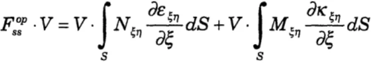
The steady state cutting force F is determined from the upper bound theorem of plasticity

FOP V = Na Sa, M dS dS (3.5)

S S

where V is the relative velocity of the plate relative to the cone, and N. and M, are the components of the membrane force and bending moment tensors. The strain and

curvature rates gap and Kap are calculated from the deformation modes described in

(27)

figure 3.3. The integration occurs over the whole deformed region. The material is characterized by the flow stress a 0.

In the local curvilinear coordinate frame shown in figure 3.4 the condition of steady state is expressed mathematically as

V = d~ (3.6)

dt

Using the chain rule and equation (3.6) we obtain

d( )=

d =v.(

)

(3.7)

dt

And now we can eliminate differentiation with respect to time from the statement of the upper bound theorem of plasticity by substituting the result of equation (3.7) into equation (3.5). Hence

FSP V= V .JN

a"

dS + V. M

dS(38)

s s

In equation (3.8), the first term of the right hand side corresponds to the membrane energy dissipation in the tip and transition zones, whereas the second term represents the energy

dissipated via bending of the curved flaps.

Additionally, the following kinematic assumptions shall be made in order to simplify the problem:

1. Small bending effects in the near-tip zone are neglected 2. Plastic shear strain is ignored

3. Local necking in the near-tip zone is ignored, and the plate thickness is taken as constant.

4. The plate material obeys a plane stress von Mises yield condition

(28)

where a=, ay and ry, are the in-plane components of the stress tensor. The corresponding flow rule is

E = (2, - yy),

yy =

i

(2a. -a ),

* 3

£,y =3Cy

(3.10)

where A is a scalar multiplier.

5. The plastic coupling between the bending moment Ma and the membrane force

Na, is neglected in the near-tip zone and the transition zones. This assumption will

overestimate the actual energy dissipated.

Making use of the above assumptions, let us now investigate the contributions of the different energy dissipation mechanisms in the curved flap model.

3.3.1.3 Bending Energy Rate

In the steady state cutting of the outer plate, bending is confined to the two inclined plastic moving hinges located in the transient flaps. The integration is performed over the

area 1, x 1, containing the diagonal line OP as shown in figure 3.4, where 1, and l,, are the projections of the hinge length I into the and rl directions, respectively. In the local coordinate system dS = dxdl, and the limits of integration become 0 < < 1 and 0 < r < ,. Also, from the geometry of the problem in figure 3.5

1, =B +Rcoso (3.11)

Let us consider one of the transient flaps in figure 3.4 and integrate first in the streamline direction 4 the second term of the right hand side of equation (3.8). Thus

ln 14

Eb =

VJJ

M d d = V M [Ktl]

d7

(3.12)

00 0

(29)

where [g] is the curvature tensor jump across the hinge line. Due to the fact that the transient flaps form a cylindrical surface, there are no variations of the curvature jump in the circumferential direction Tr. Hence

Eb = V Mn[Kr

]

(3.13)

In the local coordinate system of the cylindrical transient flaps the curvature tensor is

Ken =[iRcos6

1 (3.14)

where R is the unknown radius of the stable flaps. It follows from the geometry of figure 3.4 that the radius of the transient flaps is obtained by dividing R by the cosine of the split angle 0, as is done in equation (3.14). Finally, substituting the results of equations (3.11) and (3.14) into equation (3.13), and taking into account that there are two transient flap zones in the model we obtain

Eb

=

2

VM (B+Rcos

(3.15)

where MO is the only non-zero component of the fully plastic bending moment tensor, in the circumferential direction; 0 is the split angle and the cone angle. Using the yield condition described in equation (3.9) on the one-dimensional strain rate field we can express the yield moment MO in terms of the average flow stress a_o , which is a well documented material property. Thus,

2 t2

(30)

-3.3.1.4 Near Tip Zone Membrane Energy Rate

In the curved flap model, membrane energy dissipation occurs both in the near-tip zone and also at the transition zones. In the near-tip plastic zone the following assumptions can be made, as suggested by Zheng [4]:

1. The strain rate component in the direction of the cone shaped wedge ecg should be zero. Otherwise, material would accumulate on the wedge tip, a hypothesis which contradicts experimental observations.

2. As a consequence of kinematic assumption (2) in section 3.3.1.3, the shear component

eon is also zero.

If we now apply the above kinematic restrictions to the yield condition in equation (3.9), and its corresponding flow rule relations in equation (3.10), we obtain

A

ofa[ 0 2] (3.17)

And by virtue of the chain rule and steady state conditions in equation (3.7), the strain rate tensor is

El=

_{0 V}as(3.18)

[o (3.18)

Next, we consider the contribution of the near-tip zone membrane energy dissipation E to the first term of the right hand side of equation (3.8). Hence

Eml

=

Nse

4dS=tJ

C 4n

dS

(3.19)

s s

where N7 = t an and t is the plate thickness. The area of integration S is defined by the length of the near-tip plastic zone 1p in the streamline -direction, and by the

(31)

boundary (4) in the r-direction. Then, substituting equations (3.17) and (3.18) into (3.19)

vaI

Va~t

(3.20) >=

)

tTofV f7 dS ., .3 V d

Recall the definition of the strain rate tensor e r,

* 12 .,

E4 =7 ~2 U4+Un,4 V _{1 (U4,17}( (3.21)

Substituting equation (3.21) into equation (3.20) we obtain

km,( ) _(3.22)

where u, denotes the relative displacement in the near tip plastic zone. The maximum and

minimum displacements are given by Zheng [4] and corrected by Simonsen [6] as

u,(G = Ip) = 0 = 0.317 R cos

0

(1 + 0.55 02)

U(9 = 0) =0

We can now substitute equation (3.23) into equation (3.22). Therefore,

Em = 2 co tVu o = 0.366 Vtao RcosO (1+0.55 02) (3.24) And recalling the relationship between the fully plastic bending moment and the average flow stress expressed in equation (3.16), we arrive at the following expression for the contribution of the near tip plastic zone to the membrane energy dissipation:

to./)

km

P+(I 1 0 -~3 0 2 ,--cn V e · · D

tv 1 d (U,

d5

(32)

Em1 = 127 MO V Rcos (1+ 0.55 2) (3.25)

t

3.3.1.5 Membrane Energy Rate in the Transition Zones

The transition zones between the transient and the stable flaps are in effect toroidal surfaces where the material is first stretched and finally compressed upon entering the stable flaps. In such transition zones, the following kinematic assumptions are suggested by Zheng [4]:

1. Due to rotational symmetry of the shell, the shear strain E,7 vanishes.

2. The arc length of the transient flaps is equal to the arc length of the stable flaps. 3. The material is inextensible in the circumferential direction, i.e. e,, = 0.

After applying the above kinematic restrictions to the yield condition in equation (3.9) and the corresponding flow rule of equation (3.10), the stress and strain rate tensors become

_1

[2

(3.26)

and

e

=

oV (3.27)

O O

Next, we let us consider the contributions of the two transition zones to the membrane energy dissipation term in the right hand side of equation (3.8). Hence

Em2

=

2 N 4 dS = 2

t

ca

E dS (3.28)

S S

where Ns = t a in and t is the plate thickness. The area of integration S is defined in

the local coordinate system by the streamline coordinate boundary C and 0 < 7 < Il in the

(33)

circumferential direction, where In is defined in equation (3.11). Then, substituting

equations (3.26) and (3.27) into (3.28)

17 ?C SdE

d di7

=2t-V 4

e

o

dn

The strain in the transition zones was calculated by Zheng [4] and corrected by Simonsen [6] for a similar geometry as

e (r) = 0.29 0

sin0

cos 0/2

cos R (3.30)

After substituting for the strain into equation (3.29) and integrating we obtain

Em2 = 116 V Mo 0 sin0 coS 0/2

cos 0

(R cos + B)2

Rt

(3.31)

where Mo is defined in equation (3.17).

3.3.1.6 Theoretical Outer Plate Steady State Cutting Force without Friction

Having so far calculated the contributions of the different energy dissipation modes, we can now substitute from equations (3.15), (3.25) and (3.31) into the expression for the

steady state upper bound theorem of plasticity in equation (3.8). Hence

FP

B +

R cos b

=2.

MO R cos

+

27 R

t

Cos (1 + 0.55

02) + l16 Osine cos 0 /2 cos 0

(Rcos + B)

2

Rt

(3.32)

where we have eliminated V and have non-dimensionalized by the fully plastic bending moment M0. In equation (3.32) the unknowns are the outer plate cutting force FO, and the stable flap rolling radius R and the wedge shoulder B, both of which are defined in

E,2 =2t.

_-.F

2 (3.29)

(34)

figure 3.5. Additionally, the split angle 0 is also a free parameter which we need to determine. Therefore, at this point we have one equation for four unknowns. The immediate task is to identify another three equations relating the four unknowns.

3.3.1.7 Geometric Relation between R and B for a Conical Wedge

Figure 3.5 shows the geometry of the side view interaction between the outer plate and the cone in the curved flap model. From simple geometric arguments we can establish the following relation between R and B

h - R (1- sin)

(333)

cot

where h is the vertical distance between the vertex of the cone and the undeformed outer plate, as shown in figure 3.5. In the next section, we shall express h as a function of x. At any rate, it is sufficient to say now that h is a known quantity that can be derived from the geometry of the problem.

3.3.1.8 Closed Form Solution for the Outer Plate Steady State Cutting Force

In order to establish a third relation between the four unknowns of the problem, it is necessary to postulate that the rolling radius R adjusts itself so as to minimize the cutting force. That is, first we substitute for B from equation (3.33) into equation (3.32), and then we calculate the analytical minimum of equation (3.32), imposing the condition

dF

= 0. Then

dR

2 t_{--+ 116 sin0}1 1 6 8 cos &/2₀

R cot4 cos h cos9 Cot2 (334)

h 1 L27 cos0 (1+0.55 02) + 116 Osin COS 0/2 .[cos0 - tan (1- sin )]2

(35)

In equation (3.34), R is expressed as a function of h, which is a known geometric quantity. Therefore, we can now substitute from equations (3.33) and (3.34) into equation (3.32) and eliminate B and R as unknowns variables, leaving the plastic force FP as a function of the split angle 0 only.

3.3.1.9 Friction Contribution to the Outer Plate Steady State Cutting Force

The next step in our derivation is to include the effect of friction on the plastic cutting force. Such an effect was investigated by Zheng [17] and perfected by Pippenger [5], who found a friction correction factor for a problem of similar geometry of the form

af1 = 1+ 3 cot8 (3.35).

/2 cos 0 Cos

1-

cos

cos 0 sin 0 + t cos 0

The total plastic force is then found by multiplying equation (3.32) by equation (3.35) such that

Tot Fs° = F p f (3.36)

Let us recall that after the last few substitutions performed into equation (3.32), we have reduced the number of variables, so that FP = f(O,h(x)) only. Hence, the final step consists of determining a relation between the total force in equation (3.36) and the plate split angle 0. In figure 3.6, the total plastic force including the friction effect is plotted against the split angle 0. It is postulated that the split angle is such that it minimizes the total force. From the graph in figure 3.6, it can be inferred that the optimum split angle is 10 degrees. However, because of the transverse framing, it is impossible to conceive geometrically a crack tip far enough ahead of the cone to possibilitate such a small split angle. Hence, based on geometric constraints, a minimum split angle of 20 degrees is postulated. In figure 3.6, we observe that at 20 degrees the force level is a quasi-minimum, and therefore the violation of the criterion of minimum force for the selection of the split angle is of small order. Consequently,

(36)

outer platesteady-state = 20 deg (3.37) optimum

Finally, we have eliminated the unknown parameters B, R, and 0 , such that now FOPis a function of known geometric parameters, e.g. h, only. The geometric characteristics of

FOPare explored in the next section.

3.2.2 Geometry of Outer Plate Steady State Cutting

In section 3.2.1, the governing equation for the contribution of the steady state cutting of the outer plate to the total resisting force was derived as equation (3.36). The task now is to find the dependency of this theoretical force with respect to the distance traveled by the structure relative to the cone. In other words, the task is to establish the history of the force in order to compare it to the experimental results of the NSWC grounding experiment shown in figure 2.4.

First, let us define a coordinate system for the problem. Such coordinate system is shown in figure 2.5, where the origin O corresponds to the location of the axis of the cone at the time of the first contact with the leading edge of the structure. The y-axis runs parallel to the cone axis, and the x-axis is parallel to the ground. By symmetry, we will consider that

the cone advances with respect to an stationary structure, whereas in reality the process occurs viceversa.

Having defined the coordinate system, let us now be concerned with establishing the x-coordinate dependency of the parameters that determine the resisting force in equation (3.36), namely the flap rolling radius R and the wedge shoulder B. In equation (3.33), it was shown that B and R are related via the quantity h, the vertical distance from the vertex of the cone to the undeformed outer plate. Because of the tilt angle ca, h becomes a function of x. Then, by virtue of equation (3.33), both B and R also become functions of x. Hence, the outer plate steady state cutting force in equation (3.36) is a function of x.

Consider figure 2.5. In the x-y plane, the outer plate is described by the line

(37)

p = m - x tana

,

Xto <X < Xtl

where is the tilt angle of the plate relative to the ground, x is the location of the leading edge of the outer plate, and x mll is the location of the trailing edge of the outer

plate, as shown in figure 2.5. From geometrical considerations, the y-intercept ml can be expanded as

m = A + (d-e)(sina tan - cos a) + rtan

tan

(3.39)

where all the geometric parameters are given in table Al. Substituting from the values in table Al into equation (3.39), we obtain

m = 25.375 inches. (3.40)

From the geometry of the problem h can be defined as

h = A-yo =A-m +x tana

(3.41)

after substituting for yop from equation (3.38). Note that the height of the cone A and the height of the cone shaped rock are different because of the rounded tip of the rock. In fact, we can relate both quantities from simple geometry such that

A

l

=A+r1

sin

(3.42)

where r is the rounded tip radius and 0 the cone angle. The values for both A and A1 are listed in table Al as 38.9 inches and 36.0 inches, respectively.

Thus, we have determined h as h(x), and having done so we can substitute into equation (3.33). Then, we have expressed the total force as a function of x only, which can easily be implemented in the computer.

(38)

3.2.3 Outer Plate Steady State Cutting Boundaries

Because of the geometry of the problem as shown in figure 2.5, rupture of the outer plate occurs immediately after contact is made between the cone and the outer plate leading edge. Thus, before the process reaches steady state, a certain degree of cutting initiation is to be expected, Zheng [17]. In the present analysis, the length of the initiation phase is assumed to be the distance from point O to station x1 in figure 2.5. In other words, steady

state cutting of the outer plate begins at the point of contact between the cone and the first transverse frame.

In addition, the final location after which the steady state force drops linearly to zero is assumed to be the location of the cone axis when the cone is tangent to the outer plate trailing edge, i.e. station xj1 in figure 2.5.

By considering the geometry of figure 2.5, we can expand the boundary points xiP and op

X as

x

°P _{= X}

1

=

C2(Cos

a -

sin

a

tan )

(3.43)

xp = x = I (cos a - sin a tan e)

Substituting for the numerical values of the various parameters from table Al, we obtain

x

°P _{= 24.16 inches and}_x P

= 134.6 inches.

Li f

(39)

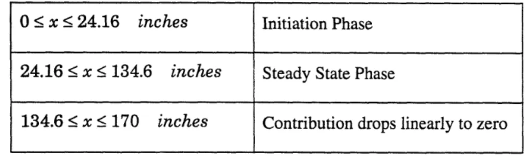
3.4 Summary of Outer Plate Contribution to the Total Resisting Force

In this chapter we have investigated the contribution of the outer plate to the total resisting force in both initiation and steady state modes. This contribution is plotted along

the length of the model structure in figure 3.7. Note that in figure 3.7 we can distinguish the following intervals:

Table 3.1: Summary of Outer Plate Contribution to the Total Resisting Force

In table 3.1, the final value of 170 inches corresponds to the overall length of the model structure. We observe that the initiation force is proportional to the square root of x, as we should expect from equation (3.1). However, the steady state component is linear with x. Such a linear dependence is also expected from the theory developed in the previous section. Recall from equation (3.41) that h is linear in x. Also, via the geometric relation in equation (3.33), B and R are linear in h, and hence linear in x. Finally, considering equation (3.32) we conclude that since the steady state force is linear in B and R, it should also be linear in x.

All calculations were performed using MATLAB software. A hard copy of the source code is included in the Appendix.

0 < x < 24.16 inches Initiation Phase

24.16 < x < 134.6 inches Steady State Phase

(40)

C~-9I-,

Fa

Figure 3.1. Aerial View of Cone Cutting through Outer Plate

40 - 4 i I I II i I

(41)

Outer Plate Initiation Force vs. Split Angle 5 4.5 4 3.5 0 a 3 2.5 1 2 1.5 0.5 10 20 30 40 50 60 70 80 90

Split Angle in [deg]

3.2. Outer Plate Initiation Force vs. Split Angle x 104

n

(42)

L. u E sw

v

10 O *_a: 10 4) L. 960 0 C0

0

_{O n} I .. AC_¢ p II v .an

(43)

la 0 CUow 0 CU Q₀ w .r To cn O-, eer cn 10 Lo O * 14 LW

(44)

..*. ...

Figure 3.5. Side View of Cone-Outer Plate Interaction

44

(45)

x 10O 0 U T E R PLATE Steady State Force vs Split Angle for constant penetration

10 20 30 40 50 60 70 80 90

Cone Split Angle in [degrees]

Figure 3.6. Outer Plate Steady State Force vs. Split Angle 8 7 6 "0 5 0 .C

04

LL 03 2 1 n 0

(46)

-

x 105

_{X ..}

OUtr Ptan

,,r_:

..

CZ-.= . a)

0

0 IL=_a) C-_o L-._ C) a.C₎ C: ( , v,., I -u 140 x-coordinate in [inches]

Figure 3.7. Theoretical Outer Plate Contribution to the Total Resisting Force

46

(47)

Chapter 4 Contribution of Inner Plate to the Total

Resisting Force

4.1 Introduction

The mechanics of the cutting process of the inner plate are significantly different from the outer plate because of the geometric configuration of the structural model. In the case of the outer plate, the proposed theoretical model developed in chapter 3 was a curved flap model. The reasoning for such a choice of model was based on the fact that rupture of the outer plate is immediate upon contact, and hence the problem becomes analogous to that of a wedge indentation through a plate.

In the case of the inner plate, however, rupture is by no means immediate. As shown in figure 2.5, the leading edge of the inner plate is higher above the ground than the tip of the cone at the initial point of contact. As the cone penetrates the structure, it begins to approach the inner plate because of the tilt angle of the plate. Eventually contact is made at the location x. From this point on, the cone pushes up the inner plate until the upward penetration generated strain reaches critical value. At this point x, rupture occurs, relieving much of the inner plate resisting force.

In addition, experimental evidence gained from NSWC Grounding Tests corroborates that the initiation of rupture in the inner plate is generated through cracks propagating ahead of the cone in the outer plate, and running up through transverse frames to meet the inner plate. In fact, according to NSWC experimental observations [1], inner plate rupture

(48)

occurs when the vertical penetration of the cone into the inner plate exceeds 0.4 times the double hull height.

After the initial point of rupture xr, the inner plate enters a steady state cutting phase, in a manner analogous to the outer plate. However, in order to capture the failure behavior described above, it is necessary to consider a different approach for the derivation of the governing equation of the steady state inner plate contribution to the total resisting force. This new approach is based on a straight flap model.

In this chapter, we shall develop theoretical models for both phases of the inner hull cutting process.

4.2 Inner Plate Cutting Initiation

4.2.1 Inner Plate Cutting Initiation Governing Equation

Consider the frontal view of the structure in figure 4.1. We observe that the vertical penetration into the inner plate is constrained by the presence of the longitudinal girders A and B. We can define the angle [5 as

tang = (4.1)

d

where is the penetration into the inner plate and d is the double hull height, which is approximately also half of the horizontal separation between the longitudinal girders. Under fully plastic conditions, the resisting force can be expressed, as derived by Simonsen [6], as

Fip = co t (4.2)

FLP(T, tS

(4.2)

Cos a

where t is the plate thickness, and the fully plastic load is projected onto the horizontal by dividing by the cosine of the tilt angle or. Finally, by including the appropriate friction correction factor into equation (4.2) we obtain

(49)

1

Cos a (sin~a + 1 +g4 cos(a +))

X < X < Xr

where the friction coefficient =0.3, x is the initial contact point between the cone and he inner plate, and xr is the point at which the inner plate ruptures.

4.2.2 Geometry of Inner Plate Cutting Initiation

In determining the geometry of the inner plate cutting process, the goal is once more to establish the variation of the force along the length of the structural model. As for the case of the outer plate, we will once more refer to the coordinate system in figure 2.5. Then, we can describe the inner plate in the x-y plane by the line

Yip

= m2

- x

tana

, to, < X < Xt12

where oa is the tilt angle, and xto. and xtl2 are the leading and trailing edges of the inner

plate. From the geometry of figure 2.5, the y-intercept m2 can be expanded as

m2 =

A

1

+(d-e)(sina tan-

cosa) +-+

r( co

COS a COS

- tan ) tan a

where all relevant geometric parameters are defined in figure 2.5 and their values given in table Al. Substituting from table Al into equation (4.5) we obtain

m2 =

40.25 inches

(4.6)

Now, we can express the penetration into the inner plate 5 as a function of x, since

S=

Al -yp

=

A

1-m2

+x tana

(4.7)

where A is the height of the cone (not the height of the rock).

Fp _=

( t

Cos

a

(4.3)

(4.4)

(50)

If we now substitute for 6 from equation (4.7) into equation (4.3), we will have expressed the force as a function of x.

4.2.3 Inner Plate Cutting Initiation Boundaries

The contribution of the inner plate cutting initiation to the total resisting force starts at the point where the cone first makes contact with the inner plate. This location can be derived geometrically from figure 2.5 as

XC

=rI1

tan-csa

1+ d +(d-e)cosa tan

-

(4.8)

cos

tan a

sina

tan

a

Substituting from table Al we calculate

x, = 33.16 inches (4.9)

Empirical observations on NSWC tests revealed that rupture occurred when the penetration exceeded 0.4 times the double hull height. This condition is expressed

mathematically as

6 = (0.4) d (4.10)

Substituting for 6 into equation (4.7) and solving for x we obtain

(0.4) d- Al + 2 (4.11)

x

r

_{tan a}

=

(4.11)

and substituting from table Al we calculate

Xr = 78.15 inches (4.12)

(51)

4.3 Inner Plate Steady State Cutting

4.3.1 Derivation of Inner Plate Steady State Cutting Force 4.3.1.1 Straight Flaps Model Kinematics

The deformation pattern of the inner plate observed in the NSWC Grounding Experiment cannot be accurately described by the curved flaps model used for the outer plate (see section 3.3.1.1). In the case of the inner plate, experimental evidence corroborates that the generated flaps do not roll away from the cone. Based on this fact, a new approach in the form of a straight flaps model was implemented.

The characteristic geometry of the straight flaps model is depicted in figure 4.2. The deformation of the inner plate is symmetric on both sides of the cone, hence only one side needs to be considered for analysis. As the plate moves past the cone with a certain velocity V, it eventually ruptures at the center, so that the line OQRS defines a free edge. The area enclosed by OPRQO is assumed to undergo plastic membrane strains with rupture.

A material streamline is shown in figure 4.2. At any given point along the trajectory, a local coordinate system is defined, where the coordinate 4 is directed in the streamline direction and the coordinate rl is perpendicular to the streamline direction. The material element is undeformed until it reaches the line OP. The, as the material element passes through the triangular region OPR, it is stretched. As discussed by Zheng [4], it is unlikely that the plate recompress to a straight flap, but rather it will tend to buckle as

shown in figure 4.2.

4.3.1.2 Energy Dissipation

Because of the large membrane strains present in the triangular region OPR in figure 4., the bending energy dissipated by the hinge line OP becomes a second order effect, and hence it shall be ignored. Hence, the statement of the steady state upper bound theorem of plasticity in equation (3.6) becomes

(52)

F'P V=V = N4, d4jdS (4.13)

S

Note that in equation (4.13) the bending energy dissipation term has been omitted in accordance to the assumption stated above.

Furthermore, let us assume that lengths of the lines PR and PQ are equal and that the transverse component of strain in the 11 direction vanishes. Shear strain is considered via an equivalent strain rate formulation. Therefore, the two dimensional strain rate tensor under the steady state condition in (3.5) becomes

*·eq

= V

a

[ eq (4.14)

Next, if we substitute for the strain tensor into the von Mises yield condition in equation (3.7) we obtain

1 F2 01

No= ta = t

a

=

t

(4.15)

Now we can substitute from equations (4.14) and (4.15) into (4.13). Thus

max+C 4 ma_x

2 e 4

Fw

= 2

~

co

t |

|

q

d

r

T=

ot

Eeq

(77)

d

(4.16)

o -c o0

where the factor of 2 comes from considering the 2 flaps on both sides of the cone. If we assume a buckled flap wake and therefore neglect strain reversal, we can express the strain as

eq (7) = () (4.17)

l(7)

(53)

where u(rj) is the stretching given by the gap between PR and PQ in figure 4.2, and l(r7) is the original length of the fiber being stretched. From the geometry of figure 4.2, we can expand the gap opening and the fiber length as

l(1) = cot 0

u(/) = /j(1- cos i)2 sin2 0 + (1- cos 0)2 sin2 (4.18)

where is defined in equation (4.1), and ilm = is the length of the straight flap tan

0

attached to the cone. Substituting from equations (4.18) into (4.17) and (4.16), and integrating we obtain the expression for the steady state inner plate cutting force as

F.P=, y t an

(tan2

+ 14)[(1-

os

)2sin 2 +(1-cos0) 2sin2 ]i (4.19)

where we have applied the relevant functional relation for the equivalent strain in equation (4.17), as suggested by Simonsen [6]. Also, in this case, the angle , i.e. the rotation of the flaps with respect to the horizontal, is constrained by the cone angle

4,

such that since the flaps are attached to the cone P=O, as shown in figure 4.3.

4.3.1.3 Friction Contribution to the Steady State Cutting Force

The friction correction factor used for the steady state cutting of the inner plate is the same as the one used for the outer plate in equation (3.35). Therefore, the total inner plate resisting force becomes

Tot F P = F~iP (4.20)

1-cos 0 sin 0 + A 1-cos 0

4.3.1.4 Closed Form Solution for the Inner Plate Steady State Cutting Force

In equation (4.20) the inner plate cone splitting angle 0 is an unknown parameter. In order to eliminate 0 as an unknown, we plot the total inner plate force in equation (4.20)

(54)

with respect to 0 . This plot is shown in figure 4.4, from which we can observe that there is no value of 0 that minimizes the total inner plate force, other than zero, the trivial solution. Thus, we are forced to estimate the splitting angle from the geometry of the steady state cutting of the inner plate. In reality, the splitting angle is constrained by the presence of transverse framing. From geometry, the average cone radius that is seen by the inner plate is on the order of half the distance between transverse frames. Therefore, a good estimate for 0 can be obtained by considering the triangular region limited by the cone radius seen by the inner plate and the transverse framing spacing, in the ratio of 1:2. In other words

tan 6inner plate t inner plate = 26 deg (4.21)

optimum 2 optimum

4.3.2 Geometry of Steady State Inner Plate Cutting Force

Let us now introduce equation (4.21) into (4.20), therefore leaving the total inner plate steady state force as a function of 5 only, which is a function of x by virtue of equation (4.7). Hence, the inner plate steady state cutting force becomes a function of x only.

4.3.3 Inner Plate Steady State Cutting Boundaries

The steady state inner plate cutting contribution begins at the point of rupture defined in equation (4.12). In addition, the final location after which the steady state force drops to zero is assumed to be the location of the cone axis when the cone is tangent to the inner plate trailing edge, i.e. station x1 2 in figure 2.5.

By considering the geometry of figure 2.5, we can expand the boundary points x and

Xf as

x p x =x

=78.15

inches

(4.22)

=

[

+

d tan(a +

)](cos

a - sin a tan )

=

1514

inches

where all parameter values are taken from table Al.

(55)

4.4 Summary of Inner Plate Contribution to the Total Resisting Force

The contribution of the inner plate to the total resisting force is plotted in figure 4.5, where we can distinguish the following intervals:

Table 4.1: Summary of Inner Plate Contribution to the Total Resisting Force

In figure 4.5, we observe that the cutting initiation behavior is quasi-linear with respect

1

to the coordinate x. The lack of perfect linearity is due to the factor in equation

cos a

(4.3). Recall from equation (4.1) that the relation between

P

and the penetration involves a trigonometric transformation. Hence, even though is linear in x by virtue of equation (4.7), 3 is only quasi-linear. Therefore , we should expect the inner force contribution to be only quasi-linear, as is the case in figure 4.5. The steady state component, on the other hand, is perfectly linear in x, as in the case of the outer plate. An interesting feature of the plot in figure 4.5 is the force drop occurring at the rupture point. This is due to the sudden release of the transverse strength, and the transition from the initiation mode to the steady state mode.

O < x < 33.16 inches No contribution

33.16 < x < 78.15 inches Inner Plate Cutting Initiation

78.15 < x < 15114 inches Inner Plate Steady State Cutting

(56)

jinner

pliating

--- tongitudina cone

L\/outer

plating

~/ ~~~ , ZH ;,\, V, F

Figure 4.1. Inner Plate Cutting Initiation Geometry

56

- Z r

J I -

-m c i e (: -_

(57)

~-2-S

(58)

Figure 4.3. Side View of Cone-Inner Plate Interaction

58

Correlation of NSWC grounding tests with MIT theory

CORRELATION OF NSWC GROUNDING TESTS

WITH MIT THEORY

Ifiigo Javier Puente

'T/2

A

-CORRELATION OF NSWC GROUNDING TESTS

WITH MIT THEORY

Ifiigo Javier Puente

Acknowledgment

Table of Contents

Force...

(53)

References

...

(84)

Appendix

...

(86)

List of Figures

List of Tables

List of Symbols

Chapter 1

Introduction

1.1 Introduction

Chapter 2

Description of NSWC Grounding

Experiment

2.1 Description of the Experimental Apparatus

2.2 Description of the Double-Hull Ship Bottom Model

2.3 Analysis of the Experimental Results

M(Vo2-Vf2)=2.0.106

ft]

dW = FH dx + F

dy

(1.3)

JFH

(X)

0

-j

0

0 H

°!l[E

:

9·-Chapter 3

Contribution of Outer Plate to the Total

Resisting Force

3.1 Introduction

3.2 Outer Plate Cutting Initiation

a -

sin a tan )

24.16 inches

3.3 Outer Plate Steady State Cutting

dt

d( )=

d =v.(

)

(3.7)

dt

dt

FSP V= V .JN

dS + V. M

dS(38)

yy =

(2a. -a ),

VJJ

d7

]

1

(3.14)

Eb

=

VM (B+Rcos

(3.15)

El=

Eml

=

Nse

4dS=tJ

C 4n

_-.F