Hydrodynamic performance evaluation of an ice class podded propeller under ice interaction

(1)

Publisher’s version / Version de l'éditeur:

Vous avez des questions? Nous pouvons vous aider. Pour communiquer directement avec un auteur, consultez la Questions? Contact the NRC Publications Archive team at

[email protected]. If you wish to email the authors directly, please see the first page of the publication for their contact information.

https://publications-cnrc.canada.ca/fra/droits

L’accès à ce site Web et l’utilisation de son contenu sont assujettis aux conditions présentées dans le site

LISEZ CES CONDITIONS ATTENTIVEMENT AVANT D’UTILISER CE SITE WEB.

27th International Conference on Offshore Mechanics and Arctic Engineering

[Proceedings], 2008

READ THESE TERMS AND CONDITIONS CAREFULLY BEFORE USING THIS WEBSITE. https://nrc-publications.canada.ca/eng/copyright

NRC Publications Archive Record / Notice des Archives des publications du CNRC :

https://nrc-publications.canada.ca/eng/view/object/?id=71b86a7f-f2b5-4da7-9c54-3caa48fcf4a2

https://publications-cnrc.canada.ca/fra/voir/objet/?id=71b86a7f-f2b5-4da7-9c54-3caa48fcf4a2

NRC Publications Archive

Archives des publications du CNRC

This publication could be one of several versions: author’s original, accepted manuscript or the publisher’s version. / La version de cette publication peut être l’une des suivantes : la version prépublication de l’auteur, la version acceptée du manuscrit ou la version de l’éditeur.

Access and use of this website and the material on it are subject to the Terms and Conditions set forth at

Hydrodynamic performance evaluation of an ice class podded propeller

under ice interaction

(2)

Hydrodynamic Performance Evaluation of an Ice Class Podded Propeller under Ice Interaction

Pengfei Liu* Ayhan Akinturk Moqin He

Institute for Ocean Technology, National Research Council, St. John’s, NL Canada A1B 3T5

Email: [email protected]

Institute for Ocean Technology, National Research Council, St. John’s, NL Canada A1B 3T5 Email: [email protected]

Oceanic Consulting Corporation

95 Bonaventure Ave. Suite 401

St. John's, NL

A1B 2X5 , Canada

[email protected]

Mohammed Fakhrul Islam Brian Veitch

Faculty of Engineering and Applied Sciences, Memorial University of Newfoundland, St.

John’s, NL Canada A1B 3X5

[email protected]

Faculty of Engineering and Applied Sciences, Memorial University of

Newfoundland, St. John’s, NL Canada

A1B 3X5 [email protected]

ABSTRACT

Fluid-structure interaction between an ice sheet on the water surface and a podded R-Class propeller was examined and analyzed in terms of numerical simulation using a newly enhanced unsteady time-domain, multiple body panel method model. The numerical model was validated and verified and also checked against various previous in-house experimental measurements. The simulation was performed in a real unsteady case, that is, the ice piece stands still and the podded propeller moves and approaches the ice piece until collision occurs. Experimental data were taken from a previous cavitation tunnel test program for a bare R-Class ice breaker propeller under open water conditions, for the R-Class propeller approaching a blade-leading-edge contoured large size ice block under the proximity condition, and from an ice tank test program for a tractor type podded/strutted R-Class propeller under open water conditions. Comparison between experimental and numerical results was made. A general agreement was obtained. The magnitude of force fluctuations during the interaction increased significantly at the instant immediately before the impact between the propeller blades and the ice piece.

INTRODUCTION

Studies of ice effects on navigation have been extensive. Ice propeller interaction is mainly divided into two broad categories: ice induced force fluctuation due to proximity, that is the suction force created between the propeller and the ice in front of it, which is called blockage effect and is hydrodynamic in nature; and, the contact force due the collision impact of ice piece on propeller and then the force on the propeller when it mills the ice [Veitch 1995]. There are some other ice conditions such as propeller blades working in a local flow domain of mixed broken ice particles and fluid. During the mid and late 1990s, some experimental investigations were also performed at the Institute for Ocean Technology and Memorial University of

Newfoundland [Doucet 1996]. In parallel with the experiments, a panel method (PM) code, or boundary element method (BEM) code, from NASA, called PMARC, was modified to simulate the ice blockage effect on propeller thrust and torque coefficients under the proximity condition (shaft thrust and torque coefficients versus different fixed gap values) [Bose 1996]. At the same time, an in-house unsteady panel method code especially targeted for propeller applications was developed [Liu 1996a], based on a boundary element method (BEM) that was developed for oscillating foil applications [Liu 1996b]. This in-house code, PROPELLA, was first used to predict the hydrodynamic effects of ice blockage in terms of the proximity, on shaft thrust, torque and normal force fluctuation of the same R-Class propeller [Liu 1996a, Liu et al. 2000]. Further, PROPELLA was modified to implement a previous ice contact load model [Veitch 1995] for the R-Class propeller. Shaft force fluctuations of several skewed ice class propellers were also obtained and analyzed [Veitch et al. 1997, Doucet et al. 1998].

In a relatively recent work, variable proximity between a wall-shaped ice blockage and the R-Class propeller was numerically modeled [Liu

et al. 2005]. In this numerical model, the ice blockage was set to

stand still whereas in the previous work the ice blockage advanced with the propeller. That is, in the recent numerical model, the propeller moves with the advance speed, approaching the ice blockage far away. A more recent experimental work was also conducted in-house for a podded ice class propeller with the same blade geometry of the R-Class propeller, except that the podded propeller is 1.5 times the diameter so the new R-Class propeller model was able to fit on a pre-tapered hub [Akinturk et al. 2003 and Wang et al. 2005]. In this experimental work, the ice blockage is a sawn ice in a notch shape, not the same as the wall-shape in the previous studies mentioned above. The current numerical work simulated this most recent experimental condition for a podded

Proceedings of the ASME 27th International Conference on Offshore Mechanics and Arctic Engineering

OMAE2008

June 15-20, 2008, Estoril, Portugal

(3)

propeller interacting with ice to observe the transient force fluctuations in this case.

PROCEDURE AND METHOD

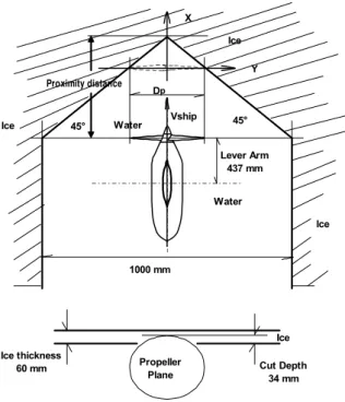
The method used in the current study is a 3-D unsteady low order panel method, in a dynamic object oriented multiple-body from. The arrangement of this form is to set objects moving in a stand-still fluid. The current numerical model was developed to simulate the ice block in front of a puller type podded propeller. Figure 1 shows the interaction scenario: the sawn ice is set to stand still in front of the podded R-Class propeller. As the diameter of the propeller is 300 mm, before the propeller approached the triangle region of the ice block, the distance from the tip of the propeller to the side edge of the ice was 350 mm (1.167R), which is greater than the diameter of the propeller, so the blockage effect of the side edge of the ice was neglected. In numerical simulation, at a time equal to zero, the propeller was aligned with the base of the ice triangle. As the triangle was equilateral with an apex angle of 90°, the vertical distance was the half of the base. Therefore, the initial distance between the propeller plane to the tip of the triangle was 350 mm. The final time step when the zero proximity occurred was when the propeller plane passed the y-axis at which position the propeller plane and the ice edge form an equilateral triangle with a base of 300 mm.

Water Ice Ice Water Ice Vship X Y 1000 mm Propeller Plane Ice Ice thickness 60 mm Cut Depth 34 mm Lever Arm 437 mm Proximity distance Dp 45° 45°

Figure 1. A SCHEMATIC DIAGRAM OF THE INTERACTION SCENARIO: A SAWN ICE NOTCH IS STANDING STILL IN

FRONT OF A MOVING AND ROTATING PODDED PROPELLER UNIT.

The new model was established on the basis of multiple body interaction. An object oriented numerical scheme was established and employed for the panel method model. In the model, the pod, strut and propeller and ice are different objects. For the perturbation potential panel method with object oriented scheme, each object has its own doublet and source influence coefficient matrix. To take into account the interaction, the body of every object is influenced by all other objects in terms of the presence of distributed doublet and source over the surfaces of all other objects.

For a detailed description of the panel method and an example of implementation of the method to a structured programming code, please refer to a text book and a PhD thesis [Katz and Plotkin 1991, Liu 1996b]. For the current multi-body formulation, each object has its own panel method system. Therefore, the numbers of the matrices to be solved in order to find the strength of the perturbation doublet potential on each panel is equal to the number of the objects in the flow field, which is different from the previous panel method that has only one doublet coefficient matrix to store all the objects in the flow domain. The interaction was taken into account, at each time step, by finding the influence of the doublet and source on the panels of all other objects and adding these influences to the right hand side of the linear equation system, as:

[ ] [ ]

[ ] [ ] [ ]

[ ]

[

] [ ] [ ]

[ ]

[

] [ ] [

]

[ ]

KNmN N w mN KN I N w JN N JN I N m K w m K I w J J I m K w m K I w I J I J J I C D C D C D C , , , 1 1 , 1 1 2 , 2 2 2 , 2 , 1 1 2 2 2 2 , 1 1 2 1 , 1 1 1 , 1 , 1 1 1 1 1 , 1 1 1 1 1 , 1 1 μ σ μ σ μ σ μ → → → → − − − − − − = M (1) where: •

[ ]

1 ₁_,₁ J I

C is the doublet influence coefficient matrix of object 1, due to a unit source strength on each of the surface panels of object 1. The subscripts I and J have the same value, i.e., the number of panels on object 1, representing the indices of row and column, respectively. The value of the elements of this matrix is dependant on the geometric shape of the local panel (centroid of a panel being influenced) and the influencing panels, and the geometrical orientation of the influencing panels. A detailed formulation and implementation procedure to determine the value of each element can be found in the above mentioned references [Katz and Plotkin 1991, Liu 1996b].

•

[ ]

1 1

J

μ is the unknown vector storing the doublet strength on the panels on object 1, which is the solution vector.

•

[ ]

1 ₁_,₁

J I

D is the source influenced coefficient matrix on the panels of object 1, influenced by the panels also on object 1.

•

[ ]

1 ₁

I

σ is the source strength equal to the normal component of the kinematic velocity at the collocation point, the centroids of the panels of object 1.

•

[ ]

1 ₁_, ₁_, ₁ m K I w

C

is the wake influenced doublet coefficient matrix of object 1 induced by the wake vortex panels shed by object 1, if object 1 is a lifting body. The subscript indices I1, K1 and

m1 stand for the number of panels on object 1, number of

vortex strips of object 1 and the number of the current time step of object 1. The variable to represent the current time step is a lower case m, as the value of m increases by one when the object advances forward for each time step. •

[ ]

1 ₁_, ₁

m K w

μ

stores the doublet strength of the wake panels on object 1, at all previous time steps. For the current time step, a steady Kutta condition is applied to obtain the doublet strength of currently shed wake panel [Katz and Plotkin 1991]. After the solution vector for doublet strength on each body panel is obtained, i.e, the solution of equation (1) is obtained, a numerical Kutta condition is performed iteratively until the pressure at the trailing edge reaches a small enough value [Liu et al. 2002].

•

[ ]

2 1 ₁_,₂

J I

D→ is the doublet influence coefficient matrix for object 1, due to a unit source strength on each of the surface panels of object 2. The subscripts I1 and J2 in most of the cases have

(4)

different values, i.e., the number of panels on objects 1 and 2, representing the indices of row and column, respectively.

• Terms in

[ ] [ ]

[ ]

2 , 2 2 2 , 2 , 1 1 2 2 2 m K w m K I w J C

μ

σ

₋ → _{are defined similarly to}

the above analogue.

It is noted that in the beginning of each time step, the solution vector for each object is obtained individually without taking into account the influence of other objects. Once the solution vectors are obtained for all the objects, the solution vectors to store the doublet velocity potential of other objects are then multiplied with the influence coefficient matrices due to other objects. The vectors as the results of the multiplication of the influence coefficient matrices for this project and the solution vectors of other objects are then added to the right hand side of this equation, as equation (1) for object 1, for instance. It is noted also that convergence study was conducted and the conclusion was that three iterations at each time step are enough to converge and in the computational runs, the iteration was set to five. When a small enough induced velocity is obtained the iteration will be stopped before it reaches five. Figure 2 shows the meshed ice block, propeller, pod and strut in the flow domain.

Figure 2. MULTI-BODY INTERACTION IN FLOW DOMAIN THAT CONSISTS OF AN ICE BLOCK AHEAD OF AN

R-CLASS PROPELLER, A POD AND A STRUT.

The advantage of the current multi-body object-oriented scheme is that it substantially reduced computing memory requirements for the doublet and source influence coefficient matrices and the CPU time that is used to inverse the matrices. For example, for the podded ice class propeller with the ice notch in the current multi-body problem, number of body and wake panels of each object is:

• Number of total panels on propeller: NTP_Prop = 3160; • Number of total panels on ice: NTP_Ice = 96;

• Number of total panels on pod: NTP_Pod = 768; • Number of total panels on strut: NTP_Strut = 576;

• Number of total wake panels on all lifting objects, in this case, on all 4 blades: 11520.

The required memory resource for individual source and doublet matrices and wake matrices is then 489 MB. While the memory requirement of the wake matrices is about the same for the single-body formulation, the requirement for the single-body panel matrices increased and hence the total memory requirement is 726 MB, about a 50% increase. This increase in the current example case is not too much to make a big difference but if the number of objects becomes large, this percentage will increase dramatically.

RESULTS AND DISCUSSION Particulars of the Propeller

Table 1 lists the particulars of the R-Class propeller along with the pod and strut geometry:

Table 1. Propeller, Pod and Strut Particulars

Propeller Particulars Pod Particulars

Diameter (m) 0.3 Overall length (m) 0.835

Number of Blades 4 Diameter (m) 0.1683

Pitch Diameter Ratio at r=0.7R

0.76 Strut Chord Length (m)

0.30 Pitch Diameter Ratio

at r=0.366R (root)

0.72 Strut Height (m) 0.2285

EAR 0.669 Aft Taper Length

(m)

0.084 Hub tape angle deg. 0 Aft Taper Shape Circular

Hub diameter 0.108 Fore Taper Angle 10°

It is noted that the taper angle of the propeller is zero. This means that the propeller end of the pod was tapered to fit the diameter of the propeller hub.

Figure 3. shows a closer view of the surface mesh of the R-Class propeller. To avoid irregular panel shape or abnormal panel aspect ratio, a uniform distribution of panels in both the chordwise and spanwise directions were used. A dense panel arrangement was obtained by taking 20 intervals in both directions.

Figure 3. SURFACE MESH OF THE R-CLASS PROPELLER.

Comparison with the Previous Results: Validation and Verification

To validate and verify the current multi-body panel method, in addition to mesh size, time step size and number of total time steps that were completed previously, propulsive performance prediction by the current method was compared with the previous ones for both open water and ice interaction cases. Predictions for this new model were only compared with the previous panel method model, along with the experimental data. Predicted unsteady hydrodynamic loads - fluctuations of propeller shaft thrust and torque were obtained and compared between the current numerical model and the previous experimental data. For the R-Class propeller, the new model agreed well with the previously published data under both the open water condition and the ice blocked flow proximity condition when approaching an ice wall contour, at which the proximity limit simulates the ultimate blockage effect as the blades are about to start to mill the ice.

The ice wall contour in front of the R-Class propeller in the validation is shown in figure 4.

(5)

Figure 4. ICE-WALL CONTOUR WITH TRAILING WAKE VORTICES IN FRONT AND BEHIND THE R-CLASS

PROPELLER IN THE PREVIOUS STUDIES. The following comparisons are made:

• Thrust and torque coefficients for the bare R-Class propeller • Thrust and torque coefficients for the bare R-Class propeller when

interacting with an ice-wall blockage

• Thrust and torque coefficients for the R-Class propeller with pod and strut

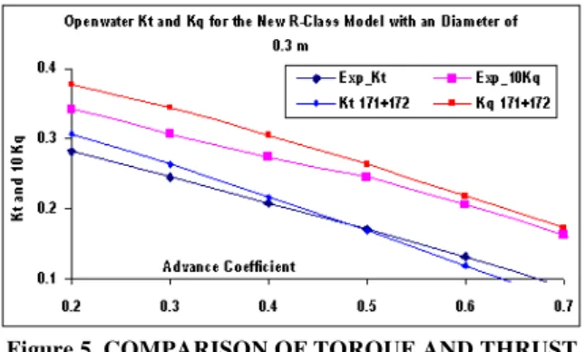
Figure 5 shows the open water thrust and torque coefficients of the R-Class propeller, obtained by the previous measurement and the current code. The current multi-body model shows a general agreement with the previous experimental work. However, at higher advance coefficients, the predicted thrust tends to be lower than the measured one and under heavily loaded conditions where the advance coefficients are near zero, the measured values of thrust and torque become lower than the predicted ones. In the computations, the interaction were set that both the body and wake panels of all other objects (object 2, … N) have a contribution to the centroid of a panel on the object under consideration (object 1), and so on. For a propeller only simulation, the number of total objects is 1, in which case the multi-body interaction iteration is not performed.

Figure 5. COMPARISON OF TORQUE AND THRUST OEFFICIENTS OF THE PROPELLER UNDER OPEN

WATER CONDITIONS.

Figures 6 and 7 compare the previously measured thrust and torque with current predicted ones, respectively, for an advance coefficient of 0.4. The abscissa is marked with the fixed proximity values in terms of percent radius of the propeller, which is 150 mm.

Figure 6. COMPARISON OF THRUST COEFFICIENT OF THE PROPELLER INTERACTING WITH THE ICE-WALL

BLOCKAGE.

The thrust comparison versus gap distance shows that the thrust drop rate for the measured data is more sensitive than the predicted ones, though the values are not very close for gap distance from 5-10% of the radius of the propeller.

Kq vs. gap in %R, Current Multiple Body Formulation 0.02 0.03 0.04 0.05 0 10 20 30 Gap %R Tor que coef fi ci ent K q multibody Kq_no-ice EXP-no-ice multibody Kq_ice 171+172 EXP1 EXP2

Figure 7. COMPARISON OF TORQUE COEFFICIENT OF THE PROPELLER INTERACTING WITH ICE-WALL

BLOCKAGE.

In figure 7, the torque produced by both the experimental and numerical work showed good agreement, especially at gap values greater than 5%R.

Comparison was also made for the R-Class propeller with a pod and strut without ice interaction and it is shown in figure 8. Again the predicted and measured torque agreed well with each other, but the measured thrust was substantially lower than the predicted.

Propulsion Performance of R-Class Puller-Type Podded Propeller (with a pod and a strut)

0.10 0.15 0.20 0.25 0.30 0.35 0.40 0.45 0.50 0.00 0.10 0.20 0.30 0.40 0.50 0.60 Advance Coefficient Kt an d 10 Kq Kt_Exp Kt__171+172 10 Kq_Exp 171+172 10Kq__171+172

Figure 8. COMPARISON OF TORQUE AND THRUST COEFFICIENTS OF THE PROPELLER INTERACTIng WITH

(6)

Shaft and Bearing Forces of the R-Class Puller Podded Propeller during Ice Interaction of Variable Proximity

In the numerical computations, a notch shaped ice sheet was implemented to approximate the model ice used during the ice tank tests. Fluid-structure interaction was simulated in terms of variable proximity only. That is, the dynamic force prediction was made before the propeller blades reached the ice cover sheet. Though there is a relatively large uncertainty caused by a very complicated interaction flow for both the experimental results and the new podded propeller numerical model, good agreement was obtained on the trend of force fluctuations for both the predictions and the measurement.

Figure 9 shows the predicted and measured thrust versus the location of the propeller’s principal axis. At a location of x=0, the propeller blades start to be in contact with the ice, where a milling process occurs but is not modeled here.

Shaft thrust coefficient flucutuation when propeller approaching an sawn ice

0.10 0.20 0.30 0.40 0.50 -80.00 -50.00 -20.00 10.00 Proximty distance (mm) Kt_Exp Kt PROPELLA

Figure 9. THRUST COEFFICIENT OF THE PROPELLER INTERACTING WITH A POD AND STRUT, UNDER

VARIABLE PROXIMITY CONDITION.

The dark line in figure 9 represents for the measured and averaged thrust coefficient values; the light points represent for the predicted thrust fluctuation marching with the time steps. The measured thrust showed a slight increase after the collision between propeller and the ice, in a magnitude slightly smaller than the maximum hydrodynamic thrust, due to a strong suction between the ice edge and the back of the propeller blade. This means that during the milling process, the shaft thrust is lower because some part of the blade that was in contact with ice did not contribute thrust but was used for cutting the ice, i.e., milling.

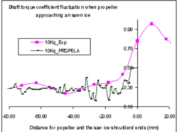
Figure 10. TORQUE COEFFICIENT OF THE PROPELLER INTERACTING WITH A POD AND STRUT, UNDER

VARIABLE PROXIMITY CONDITION.

In figure 10, shaft torque history during the variable proximity interaction is shown. From the previous experimental data, it can be seen that the maximum torque coefficient occurred immediately after the collision, and the magnitude of the maximum is about twice as big of the maximum predicted torque coefficient immediately before collision at a gap value of about zero.

Predicted torque coefficient in figure 10 agrees well with the measurements for relatively large gap values of greater than 10%R. When the two tips of the propeller blades are at the mid of the 2nd and 1st quadrant locations, the proximity effect becomes significant because of the shape of the ice notch (see figure 1 for detail).

Figures 11 and 12 show the horizontal and vertical bearing force coefficients, compared with the measured data in the previous studies. Due to sign convention, the transverse bearing force predicted and measured are opposite so that an underscore is used before the legend for the measured transverse force as “_KFy_Exp”.

Horizontal Bearing Force Coefficient

-0.10 0.00 0.10 0.20

-80.00 -60.00 -40.00 -20.00 0.00 20.00 Proxim ity distance

_KFy_Exp KFy PROPELLA

Figure 11. HORIZONTAL BEARING FORCE COEFFICIENT OF THE PROPELLER INTERACTING WITH A POD AND

STRUT, UNDER VARIABLE PROXIMITY CONDITION.

Vertical Bearing Force Coefficient

-0.25 -0.15 -0.05 0.05

-80.00 -60.00 -40.00 -20.00 0.00 20.00 Proxim ity distance

KFz_Exp KFz PROPELLA

Figure 12. VERTICAL BEARING FORCE COEFFICIENT OF THE PROPELLER INTERACTING A WITH POD AND STRUT, UNDER VARIABLE PROXIMITY CONDITION. The transverse or the horizontal bearing coefficient predicted by the current numerical model agreed well with the measured ones. It also can be seen that after collision, the measured force is about the same magnitude as the predicted maximum magnitude of the transverse

(7)

bearing force (about 20% higher after collision). The rate of increase of the magnitude of the transverse force would be larger for more contact area between the propeller blade and the ice. However, in the current case, the contact area is small because only a small portion of the blade has heavy blockage effect (suction between blade surface and the ice surface).

Comparison of the vertical force in figure 12, showed a large discrepancy at gap values of less than 15 mm, i.e., 10%R. For larger gap values, the measured and predicted magnitudes have better agreement.

Figure 13 shows the instantaneous direction of the resultant force acting on the shaft bearing. Figure 14 shows the magnitude of the resultant force coefficient.

Angle of Resultant Bearing Force Coefficient

-120 -100 -80 -60 -40 -20 0 20 40 60 80 100 -70.00 -50.00 -30.00 -10.00 10.00

Gap Variation in Time History

Angle_Exp Angle_PROPELLA

Figure 13. TRANSIENT SHAFT BEARING FORCE DIRECTION UNDER VARIABLE PROXIMITY CONDITION.

Angle of Resultant Bearing Force Coefficient

-0.05 0.00 0.05 0.10 0.15 0.20 0.25 0.30 -70.00 -50.00 -30.00 -10.00 10.00 Gap Variation in Time History

Resultant Force_Exp Resultant Force_PROPELLA

Figure 14. TRANSIENT SHAFT RESULTANT BEARING OF THE PROPELLER INTERACTION WITH POD AND STRUT,

UNDER VARIABLE PROXIMITY CONDITION. Figure 14 shows that the resultant force prediction agreed generally with the measurement and was much lower than the measured one when the blade tip touched the sawn ice.

It is noted that prediction gave a larger fluctuation shown in the figures 9-14. As the flow is fully unsteady and interactive, a moderate fluctuation is expected. Reducing the time step size, the fluctuation may be reduced. In fact, the measured experimental data has been filtered in a smooth form based on the raw data.

Numerical Prediction on Blade Sectional Pressure Distribution and Cavitation Behavior

As the flow is highly unsteady and the propeller is under a heavily loaded condition, a robust model combined with both multiple-body interaction iteration and unsteady numerical Kutta condition is

essential to obtain converged and reliable results. For numerical Kutta condition used in the current work, an advance iterative Kutta condition was developed [Liu et al. 2002] and employed, because previous Newton-Raphson based iterative Kutta worked well only for a stand-alone propeller of relatively simple geometry under lightly loaded conditions. For multiple-body interaction at low advance coefficients, converged solution cannot be obtained when the previous iterative Newton-Raphson based Kutta condition was employed. Further, as all the forces and moments acting on propeller blade and shaft were obtained by an integration of the blade surface pressure distribution, these pressure distributions are important and thus shown in figures 15-23.

In computational runs, the number of total time steps was set at 180 for three revolutions. Results were collected starting at time step at 121. Figures 15-17 show the predicted pressure coefficient at the blade section at r/R=0.5048. The pressure coefficient is defined by:

t

V

p

C

ref ref lf ref ref p

_∂

Φ

∂

−

=

−

=

2 2 2 2

2

1

2

1 v

v

ρ

(2)

where P is the pressure at the collocation point, Pref is the reference

pressure, Vref is the reference velocity of the body relative to the earth.

The right hand side of equation (2) is derived with panel method notation (see Katz and Plotkin 1991 for detail).

Cp at NTStep=144 (gap distance = 49.80 mm, blade pointing at 306 dge.) -0.6 -0.4 -0.2 0 0.2 0.4 0.6 0 0.2 0.4 0.6 0.8 1 Chord location x /C M-Body _r/R = 0.5048 IPK_r/R = 0.5048 r/R = 0.5048

Figure 15. TRANSIENT KEY-BLADE PRESSURE COEFFICIENT AT ABOUT 50% RADIAL LOCATION FOR A PROXIMITY DISTANCE OF 49.80+150=198.80 MM.

Cp at NTStep=157 (gap distance = 31.82 mm, blade pointing at 228 deg.) -0.6 -0.4 -0.2 0 0.2 0.4 0.6 0 0.2 0.4 0.6 0.8 1 Chord location x /C M-Body _r/R = 0.5048 IPK_r/R = 0.5048 r/R = 0.5048

(8)

In figure 15, the transient key-blade pressure coefficient is shown. The proximity distance is defined by the gap distance plus the distance (150 mm) between the base and the tip of the equilateral triangle in figure 1. At the 144th_{time step, the key-blade points}

downward at 306°.

In figures 15-23, three types of pressure coefficient are shown. They are r/R=0.5048, standing for the predicted pressure coefficient without multiple-body correction, M_Body_r/R=0.5048, for pressure coefficient after multiple-body interaction, and IPK_r/R=0.5048, the final correct pressure coefficient after iterative pressure Kutta condition. At the 157th time step, the key-blade points at 228° and at the 161st time step, the key-blade points at 204°.

Figures 18-20 show the predicted pressure coefficient at the blade section at r/R=0.7027.

Cp at NTStep=144 (gap distance = 49.80 mm, blade pointing at 306 dge.) -0.4 -0.3 -0.2 -0.1 0 0.1 0.2 0.3 0 0.2 0.4 0.6 0.8 1 Chord location x /C M-Body _r/R = 0.7027 IPK_r/R = 0.7027 r/R = 0.7027

Comparing the pressure coefficient values at the 50% spanwise direction, these coefficients at the 70% locations have less effect due to multiple-body interaction. However, iterative Kutta condition modified the pressure distribution substantially, especially at the trailing edge, where the difference in pressure coefficient, or the pressure, approached zero. This improved the prediction, in most

cases, especially when the iteration converges. Figures 21-23 show the predicted pressure coefficient at the blade section at r/R=0.7027.

Cp at NTStep=161 (gap distance = 26.28 mm, blade pointing at 204 dge.) -0.4 -0.3 -0.2 -0.1 0 0.1 0.2 0.3 0.4 0 0.2 0.4 0.6 0.8 1 Chord location x /C M-Body _r/R = 0.7027 IPK_r/R = 0.7027 r/R = 0.7027

(9)

Cp at NTStep=161 (gap distance = 26.28 mm, blade pointing at 204 dge.) -0.5 -0.3 -0.1 0.1 0.3 0 0.2 0.4 0.6 0.8 1 Chord location x /C M-Body _r/R = 0.9005 IPK_r/R = 0.9005

The predicted pressure coefficients at around the tip of the propeller key-blade have less effect due to multiple-body interaction though the iterative numerical Kutta condition improved the pressure dramatically.

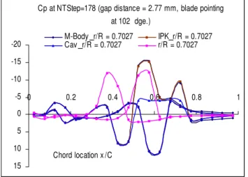
Figures 24-26 show the predicted pressure coefficients for the proximity of 150+2.77 mm, for the blade sections of about 50%, 70% and 90%, respectively. At the 178th time step, the key-blade points at 102°.

Except for figure 24, where at a smaller radial blade location, the pressure profile looks normal, figures 25 and 26 show an undesired and irregular pressure coefficient distribution at relatively larger radial locations that are close to the blade tip. In these locations, both the propeller blade suction side and pressure side have a contact with the broken sawn ice. Due to a very close distance between the blade surface elements and the panels on the sawn ice, a great jump of suction pressure was produced for the 90% blade location and for both the 90% and 70% location on both suction and pressure sides. As a result of excessive suction pressure between the ice and the propeller blade surface, cavitation was predicted and hence a more realistic pressure profile was obtained after cavitation correction (see the dark lines with triangle marks) [Liu et al. 2001].

Cp at NTStep=178 (gap distance = 2.77 mm, blade pointing at 102 deg.) -2 -1 0 1 2 0 0.2 0.4 0.6 0.8 1 Chord location x /C M-Body _r/R = 0.5048 IPK_r/R = 0.5048 Cav _r/R = 0.5048 r/R = 0.5048

Cp at NTStep=178 (gap distance = 2.77 mm, blade pointing at 102 dge.) -20 -15 -10 -5 0 5 10 15 0 0.2 0.4 0.6 0.8 1 Chord location x /C M-Body _r/R = 0.7027 IPK_r/R = 0.7027 Cav _r/R = 0.7027 r/R = 0.7027

Cp at NTStep=178 (gap distance = 2.77 mm, blade pointing at 102 deg.) -60 -40 -20 0 20 0 0.2 0.4 0.6 0.8 1 Chord location x /C M-Body _r/R = 0.9005 IPK_r/R = 0.9005 Cav _r/R = 0.9005 r/R = 0.9005

(10)

CONCLUSION

A multiple-body interaction model was established and incorporated in an in-house propeller code PROPELLA to simulate a podded R-Class propeller interacting with a sawn ice sheet, under transient proximity condition. The new model was compared with the previous experimental data as well as the previous predictions by the same code using the integrated body model (all objects were assumed to be one piece). While the current model still needs further refinement, it produced relatively reasonable results. For example, the transient shaft loading was reasonable in terms of both magnitude and direction, and hence the model could be used for hydrodynamic prediction under proximity condition, not only for ice but also for other interaction between propeller and other objects.

ACKNOWLEDGEMENT

The authors wish to thank the National Research Council (Institute for Ocean Technology) and Transport Canada for their support.

REFERENCES

[1] B. Veitch, 1995. Predictions of Ice Contact Forces on a Marine

Screw Propeller During the Propeller-Ice Cutting Process, Acta

Polytechnica Scandinavica, Mechanical Engineering Series No. 118, Espoo, Finland, 140p.

[2] J.M. Doucet, 1996. "Cavitation Erosion Experiments in Blocked Flow with Two Ice-Class Propeller Models", M.Eng. Master's Thesis, Memorial University of Newfoundland, 197p.

[3] N. Bose, 1996. “Ice Blocked Propeller Performance Predictions Using a Panel Method”, Transactions of the Royal Institutions of

Naval Architects, Vol. 138, pp. 213-226.

[4] P. Liu, 1996a. Software Development on Propeller Geometry

Input Processing and Panel Method Predictions of Propulsive Performance of the R-Class Propeller. MMC Engineering &

Research Report, NL Canada, 50 p.

[5] P. Liu, 1996b. A Time-Domain Panel Method for Oscillating

Propulsors with Both Chordwise and Spanwise Flexibility, PhD

Thesis, Memorial University of Newfoundland, St. John’s, Newfoundland, Canada, 126p.

[6] P. Liu, J.M. Doucet, B. Veitch, I. Robbins and N. Bose, 2000. "Numerical Prediction of Ice Induced Hydrodynamic Loads on Propellers Due to Blockage," Oceanic Engineering International

(OEI), vol. 4, no. 1, 2000, pp.31-38

[7] B. Veitch, N. Bose, C. Meade, and P. Liu, 1997. “Predictions of Hydrodynamic and Ice Contact Loads on Ice-Class Screw Propellers”,

Proceedings of the 16th International Conference on Offshore Mechanics and Arctic Engineering, American Society of Mechanical

Engineers, Vol. 4, pp. 119-125.

[8] J.M. Doucet, P. Liu, N. Bose and B. Veitch, 1998, “Numerical Prediction of Ice-Induced Loads on Ice-Class Screw Propellers Using a Synthesized Contact/Hydrodynamic Code”, OERC Report Number:

OERC-1998-004, Memorial University of Newfoundland, 19p.

[9] P. Liu, B. Colbourne and S. Chin, 2005. "A time-domain surface panel method for a flow interaction between a marine propeller and an ice blockage with variable proximity”, Journal of Naval

Architecture and Marine Engineering, June, Vol.2, No.1, pp. 15-20.

[10] A. Akinturk, S. J. Jones, C. Moores, 2003. “Testing propulsion systems for performance in ice”, MARI-TECH 2003, 28-30 May 2003, Montreal, Quebec, Paper 14.

[11] J. Wang, A. Akinturk, S. J. Jones, N. Bose, 2005. “Ice loads on a model podded propeller blade in milling conditions”, 24th International Conference on Offshore Mechanics and Arctic Engineering, 12-17 June 2005, Halkidiki, Greece OMAE2005-67416. [12] J. Katz and A. Plotkin, 1991. Low-speed aerodynamics, From

Wing Theory to Panel Method,, McGraw-Hill, New York, 1991, 632p.

[13] P. Liu, N. Bose and B. Colbourne, 2002. "Use of Broyden’s Iteration for an Unsteady Numerical Kutta Condition," International

Shipbuilding Progress (ISP), 49, no. 4 (2002) pp. 263-273.

[14] P. Liu, N. Bose and B. Colbourne, 2001. "Incorporation of a

critical pressure scheme into a time-domain panel method for propeller sheet cavitation,” International Workshop on Ship