The MIT Faculty has made this article openly available.
Please share
how this access benefits you. Your story matters.
Citation
Karaman, Sertac et al. "Anytime Motion Planning using the RRT*."
2011 IEEE International Conference on Robotics and Automation
(ICRA) May 9-13, 2011, Shanghai International Conference Center,
Shanghai, China.
As Published
https://ras.papercept.net/conferences/scripts/abstract.pl?
ConfID=34&Number=1887
Publisher
Institute of Electrical and Electronics Engineers
Version
Author's final manuscript
Citable link
http://hdl.handle.net/1721.1/63170
Terms of Use
Creative Commons Attribution-Noncommercial-Share Alike 3.0
Anytime Motion Planning using the RRT
∗
Sertac Karaman
Matthew R. Walter
Alejandro Perez
Emilio Frazzoli
Seth Teller
Abstract— The Rapidly-exploring Random Tree (RRT) al-gorithm, based on incremental sampling, efficiently computes motion plans. Although the RRT algorithm quickly produces candidate feasible solutions, it tends to converge to a solution that is far from optimal. Practical applications favor “anytime” algorithms that quickly identify an initial feasible plan, then, given more computation time available during plan execution, improve the plan toward an optimal solution. This paper
describes an anytime algorithm based on the RRT∗which (like
the RRT) finds an initial feasible solution quickly, but (unlike the RRT) almost surely converges to an optimal solution. We
present two key extensions to the RRT∗, committed trajectories
and branch-and-bound tree adaptation, that together enable the algorithm to make more efficient use of computation time online, resulting in an anytime algorithm for real-time implementation. We evaluate the method using a series of Monte Carlo runs in a high-fidelity simulation environment,
and compare the operation of the RRT and RRT∗methods. We
also demonstrate experimental results for an outdoor wheeled robotic vehicle.
I. INTRODUCTION
The motion planning problem is to find a dynamically feasible trajectory that takes the robot from an initial state to a goal state while avoiding collision with obstacles. Motion planning is of fundamental importance not only for robotics [1], but also in many applications outside the robotics domain [1]–[4].
From a computational complexity point of view, even a simple form of the motion planning problem is PSPACE-hard [5], which suggests that any complete algorithm, i.e., one that returns a solution if one exists and returns failure otherwise, is doomed to be computationally intractable.
In order to achieve computational efficiency, practical motion planning methods generally relax the completeness requirements. Sampling-based approaches, including algo-rithms such as the Probabilistic RoadMap (PRM) [6] and the RRT [7], form a relatively recent line of research in this direction. Most sampling-based algorithms are probabilisti-cally complete, i.e., the probability that the algorithm finds a solution, if one exists, converges to one as the number of samples approaches infinity.
Sampling-based algorithms have the advantage that they are able to find a feasible motion plan relatively quickly (when a feasible plan exists), even in high-dimensional
Sertac Karaman and Emilio Frazzoli are with the Laboratory for In-formation and Decision Systems, Massachusetts Institute of Technology, Cambridge, MA, USA{sertac, frazzoli}@mit.edu
Matthew R. Walter and Seth Teller are with the Computer Science and Artificial Intelligence Laboratory, Massachusetts Institute of Technology, Cambridge, MA, USA{mwalter, teller}@csail.mit.edu
Alejandro Perez is with the Polytechnic University of Puerto Rico, San Juan, PR, [email protected]
state spaces. Furthermore, the RRT, in particular, effectively handles systems with differential constraints. These char-acteristics make the RRT a practical algorithm for motion planning on state-of-the-art robotic platforms [8].
Any robotic motion planning algorithm intended for prac-tical use must operate within limited real-time computational resources and incomplete and imperfect knowledge of the environment. Such settings favor “anytime” algorithms that quickly find some feasible but not necessarily optimal mo-tion plan, then incrementally improve it over time toward optimality. An anytime motion planning algorithm should exhibit two properties: a form completeness guarantees and asymptotic optimality. A system based on anytime planning overlaps two functions in time: execution of (some initial portion of) its current plan, and computation to replace (any pending portion of) the current plan with an improved plan. The RRT algorithm exhibits the first property, efficiently finding an initial feasible solution. Until recently, the RRT’s ability to improve this solution as the number of samples increases was an open research question. Karaman and Frazzoli [9] proved that the probability of the RRT algorithm converging to an optimal solution is actually zero. In the same paper, they proposed an alternative method, RRT∗, a sampling-based algorithm with the asymptotic optimality property, i.e., almost-sure convergence to an optimal solution, along with probabilistic completeness guarantees. The RRT∗ algorithm achieves the asymptotic optimality absent from the RRT without incurring substantial computational overhead.
Hence, RRT∗ provides substantial benefits, especially for real-time applications. Like the RRT, it quickly finds a fea-sible motion plan. Moreover, it improves the plan toward the optimal solution in the time remaining before plan execution is complete. This refinement property is advantageous, as most robotic systems take significantly more time to execute trajectories than to plan them. For example, robotic cars [10] spend no more than a few seconds to plan a path before driving toward the goal, which may take several minutes. In such settings, asymptotic optimality is particularly useful, since the available computation time as the robot is moving along its trajectory can be used to improve the quality of the remaining portion of the planned path.
In this paper, we leverage the anytime asymptotic op-timality property of the RRT∗ algorithm to improve the online convergence of the plan during execution. Our ex-perimental results show that these proposed extensions to RRT∗ substantially improve trajectory quality. We analyze the algorithm, compare its performance to that of RRT in a realistic simulation environment, and demonstrate its effectiveness on a wheeled robotic vehicle [11]–[13].
II. THERRT* ALGORITHM
This section formally states the motion planning problem and describes the RRT∗ algorithm. Consider a system with dynamics of the following form: ˙x(t) = f(x(t), u(t)), where x(t) ∈ X and u(t) ∈ U, where X ⊂ Rdand U ⊂ Rmdenote the state space and the input space, respectively. Let Xobs
denote the obstacle region, and Xfree= X \ Xobs define the
obstacle-free space. Finally, let Xgoal⊂ X denote the goal
region. The motion planning problem is to find a control input u: [0, T ] → U that yields a feasible path x(t) ∈ Xfree
for t ∈[0, T ] from an initial state x(0) = xinit to the goal
region x(T ) ∈ Xgoal that obeys the system dynamics.
The optimal motion planning problem imposes the addi-tional requirement that the resulting feasible path minimize a given cost function, c(x), mapping each non-trivial admis-sible trajectory x: [0, T ] → X to a positive real number.
In solving the optimal motion planning problem, the RRT∗ algorithm builds and maintains a tree T = (V, E) comprised of a vertex set V of states from Xfreeconnected by directed
edges E ⊆ V × V . The manner in which the RRT∗generates this tree closely resembles that of the standard RRT, with the addition of a few key steps that achieve optimality. The RRT∗ algorithm uses a set of basic procedures, which we describe in the context of kinodynamic motion planning [14].
Sampling: The Sample function randomly samples a state zrand∈ Xfreefrom the obstacle-free region of the state space.
Distance: Dist : X × X → R≥0 returns the cost of the
optimal trajectory between two states, assuming no obstacles. Without differential constraints, it is the Euclidean distance. Nearest Neighbor: Given a state z ∈ X and the tree T = (V, E), the v = Nearest(T, z) function returns the nearest node in the tree in terms of the distance function.
Near-by Vertices: Given a state z ∈ X, tree T = (V, E), and a number n, the Znearby = Near(T , z, n) function returns
the vertices in V that are near z. More precisely, define Reach(z, l) = {z0 ∈ X | Dist(z, z0) ≤ l or Dist(z, z0) ≤ l}, and choose l(n) such that Reach(z, l(n)) contains a ball of volume γ((log n)/n)d, where γ is a fixed number [14].
Collision Check: The ObstacleFree(x) function checks whether a path x: [0, T ] → X lies within the obstacle-free region of state space, i.e., x(t) ∈ Xfree for all t ∈[0, T ].
Steering: The (x, u, T ) = Steer(z1, z2) function solves
for the control input u : [0, T ] that drives the system from x(0) = z1to x(T ) = z2 along the path x: [0, T ] → X.
Node Insertion: Given the current tree T = (V, E), an existing state zcurrent ∈ V , and a new state znew, the
InsertNode(zcurrent, znew, T) procedure adds znew to V and
creates an edge to zcurrentas its parent, which it adds to E. It
assigns a Cost(znew) to znew equal to that of its parent, plus
the cost c(x) of the trajectory associated with the new edge. Using these functions, the RRT∗ exhibits the general structure outlined in Alg. 1. With the exception of the process of extending an existing node in the tree toward a new node (lines 8–11), the RRT∗essentially behaves identically to the RRT. The RRT∗ starts with an empty tree and adds a single node corresponding to the initial state. It then builds and
refines the tree through a set of N iterations (lines 3–11). Like the RRT, the RRT∗ incrementally builds the tree by sampling a random state zrand from the obstacle-free space
(line 4) and solving for a trajectory xnew that extends the
closest node in the tree znearest toward the sample (lines 5–
6). If this trajectory does not collide with obstacles (line 7), the standard RRT inserts the new node znewinto the tree with
znearestas its parent and continues with the next iteration.
It is here that the operation of the RRT∗ differs. Rather than choosing the nearest node as the parent, the RRT∗ considers all nodes in a neighborhood of znew (line 8) and
evaluates the cost of choosing each as the parent. This process (Alg. 2) evaluates the total cost as the additive combination of the cost associated with reaching the potential parent node and the cost of the trajectory to znew. The node
that yields the lowest cost becomes the parent as the new node is added to the tree (Alg. 1, line 10). The ReWire procedure described in Alg. 3 then checks each node znearin
the vicinity of znew to see whether reaching znear via znew
would achieve lower cost than doing so view its current parent (Alg. 3, line 3). When this connection reduces the total cost associated with znear, the algorithm modifies (“rewires”)
the tree to make znew the parent of znear (line 4). The RRT∗
then continues with the next iteration. Algorithm 1: T = (V, E) ← RRT? (zinit) 1 T ← InitializeTree(); 2 T ← InsertNode(∅, zinit, T ); 3 for i = 1 to i = N do 4 zrand← Sample(i);
5 znearest← Nearest(T , zrand);
6 (xnew, unew, Tnew) ← Steer(znearest, zrand);
7 if ObstacleFree(xnew) then
8 Znear← Near(T , znew, |V |);
9 zmin← ChooseParent(Znear, znearest, znew, xnew);
10 T ← InsertNode(zmin, znew, T );
11 T ← ReWire(T , Znear, zmin, znew);
12 return T
Algorithm 2: zmin← ChooseParent(Znear, znearest, xnew)
1 zmin← znearest;
2 cmin← Cost(znearest) + c(xnew);
3 for znear∈ Znear do
4 (x0, u0, T0) ← Steer(znear, znew);
5 if ObstacleFree(x0) and x0(T0) = znew then
6 c0= Cost(znear) + c(x0);
7 if c0< Cost(znew) and c0< cmin then
8 zmin← znear;
9 cmin← c0;
10 return zmin
Algorithm 3: T ← ReWire(T , Znear, zmin, znew)
1 for znear∈ Znear\ {zmin} do
2 (x0, u0, T0) ← Steer(znew, znear);
3 if ObstacleFree(x0) and x0(T0) = znear and
Cost(znew) + c(x0) < Cost(znear) then
4 T ← ReConnect(znew, znear, T );
III. EXTENSIONS FORANYTIMEMOTIONPLANNING
This section describes how to exploit the anytime nature of the RRT∗algorithm to achieve an online motion planning algorithm that significantly improves path quality during path execution, i.e. as the robot is moving toward its goal. These extensions are inspired by techniques for real-time kinodynamic planning [8].
A. Committed Trajectory
Upon receiving the goal region, the online planning algo-rithm starts an initial planning phase, in which the RRT∗runs until the robot must start moving toward its goal. The amount of time devoted to this initial phase is domain-dependent. In the example presented in this paper involving a full-size robotic forklift, this time is on the order of a few seconds, which is the time required to put the vehicle in gear.
Once the initial planning phase is completed, the online algorithm goes into an iterative planning phase, in which the robot starts to execute the initial portion of the best trajectory in the tree maintained by the RRT∗ algorithm. Meanwhile, the RRT∗ algorithm focuses on improving the remaining part of the trajectory. Once the robot reaches the end of the portion that it is executing, the iterative phase is restarted by picking the current best path in the tree and executing its initial portion.
More precisely, the iterative planning phase occurs as follows. Given a motion plan x: [0, T ] → Xfree generated
by the RRT∗ algorithm, the robot starts to execute an initial portion of x : [0, tcom] until a given commit time tcom.
We refer to this initial path as the committed trajectory. Once the robot starts executing the committed trajectory, the RRT∗ algorithm deletes each of its branches and declares the end of the committed trajectory x(tcom) to be the new
tree root. This effectively shields the committed trajectory from any further modification. As the robot proceeds along the committed trajectory, the RRT∗ algorithm continues to improve the motion plan within the new (i.e., uncommitted) tree of trajectories. Once the robot reaches the end of the committed trajectory, the procedure restarts, using the initial portion of what is currently the best path in the RRT∗ tree to define a new committed trajectory. The iterative phase repeats until the robot reaches the goal region.
B. Branch-and-Bound
In addition to considering a committed trajectory, we also employ a branch-and-bound technique to more effi-ciently build the tree. Branch-and-bound is used within many domains in optimization and artificial intelligence. Most notably, the approach we present in this section shares certain aspects with the A∗ graph search algorithm and its variants, which are widely used in robotics applications [15].
1) Cost-to-go functions: Before providing the details of the branch-and-bound algorithm, let us first define a cost-to-go function as follows. For an arbitrary state z ∈ Xfree, let
c∗z be the cost of the optimal path that starts at z and reaches the goal region, Xgoal. A cost-to-go function CostToGo(z)
associates each z ∈ Xfree with a real number between 0
and c∗z. Essentially, CostToGo(z) provides a lower-bound
on the optimal cost to reach the goal from z. The cost-to-go function described here is equivalent to the admissible heuristic employed by A∗ planning algorithms.
There are many ways to define a cost-to-go function, the most trivial being CostToGo(z) = 0 for all z ∈ Xfree.
Note that as the cost function more closely approximates the optimal cost-to-go c∗z, the branch-and-bound algorithm becomes more effective.
In this paper, we use the Euclidean distance between z and Xgoal (neglecting obstacles) divided by the maximum
speed of the vehicle as a cost-to-go function.
2) Branch-and-bound algorithm: In the context of the RRT and RRT∗, the branch-and-bound algorithm works as follows. Let T = (V, E) be a tree and z ∈ V be a vertex in T . Recall that Cost(z) denotes the cost of the unique path that starts from the root node and reaches z through the edges of T . Let zmin be the node that lies
in the goal region and has the lowest-cost trajectory that reaches Xgoal along the edges of T . The cost of the unique
trajectory that starts from the root and reaches zmin gives
an upper bound on cost. Let V0 denote the set of nodes z for which the cost to get to z, plus the lower-bound on the optimal cost-to-go, is more than the upper-bound cu, i.e.,
V0= {z ∈ V | Cost(z)+CostToGo(z) ≥ Cost(zmin)}. The
branch-and-bound algorithm keeps track of all such nodes and periodically deletes them from the tree.
IV. SYSTEMDYNAMICS ANDTHECONTROLPROCEDURE
This section, outlines the aforementioned steering function and trajectory controller employed by the RRT∗.
A. Dubins Curve Steering Function
The RRT∗ algorithm uses a steering function that assumes a Dubins vehicle model [16] to generate dynamically-feasible trajectories for curvature-constrained vehicles. Dubins vehi-cle dynamics have the general form:
˙xD= vDcos(θD)
˙yD= vDsin(θD)
˙θD= uD, |uD| ≤
vD
ρ ,
where(xD, yD) and θDspecify the position and orientation,
uD is the steering input, vD is the velocity, and ρ is the
minimum turning radius.
There are six types of paths that characterize the optimal trajectory between two states for a Dubins vehicle, each specified by a sequence of left, straight, or right steering inputs [16]. In this paper, we consider four path classes and choose the steering between two states that minimizes cost. Karaman and Frazzoli [14] describe the steering function in more detail.
B. Trajectory Tracking
The steering function returns a trajectory parametrized by a sequence of reference states (xR, yR, θR) and a
ref-erence velocity vR. We employ a straightforward steering
Let zn be the robot’s current state and zn+1 be the next
reference point. Define the cross-track error ect be the
dis-tance between zn and zn+1 along a line perpendicular to
the desired orientation θn+1. We steer the vehicle along the
trajectory by controlling the steering angle δ via δ= Kstr arctan(Kctect) + Kstreθ,
where Kstr and Kct are gains. Meanwhile, we employ a PI
controller to track the reference speed vR,
u= Kp(vR− v) + Ki
Z t
0
(vR− v(τ)) dτ.
Using these controllers, the robot tracks the trajectory defined by the sequence of reference points.
V. RESULTS
We implemented our algorithm in simulation as well as on an outdoor ground vehicle. In this section we discuss the performance of the RRT∗ in both domains and compare the results against those of a standard RRT. The simulations demonstrate the algorithm’s ability to exploit computation available during the execution of the committed trajectory to improve the solution. In contrast, while RRT may improve the trajectory by chance through constant re-planning, such improvements are unlikely (probability zero convergence). A. Performance Analysis
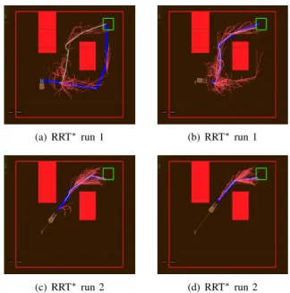
We first evaluate the implications of execution-time re-planning for the RRT∗using a high-fidelity vehicle simulator. The vehicle dynamics correspond to those of a rear wheel-steered nonholonomic ground vehicle. Shown in Fig. 1, the environment consists of a bounded region with two polygonal obstacles. The planner must find a feasible trajectory from an initial pose in the lower left of the environment to the goal region indicated by the green box. We performed a total of 166 Monte Carlo simulation runs with the RRT∗ motion planner and 191 independent runs with the standard RRT. Both planners use branch-and-bound for tree expansion and maintain a committed trajectory. Both the RRT and RRT∗ were allowed to explore the state space throughout the execution period.
Figure 1 depicts the result of two independent runs of the RRT∗ in the simulation environment. In the first, the RRT∗ initially finds a trajectory that takes the vehicle along a relatively high cost path to the right of the obstacle (Fig. 1(a), in blue). As the vehicle begins to execute the plan, however, tree rewiring reveals a shorter, lower-cost route between the obstacles (Fig. 1(b)). Meanwhile, the second run demonstrates the benefit of branch-and-bound and online refinement as the algorithm improves the current path (Fig. 1(c)) into a more direct path to the goal (Fig. 1(d)).
We compare the paths executed by the RRT∗ with those that result from a standard RRT-based planner. Figure 2 shows two different runs of the RRT at different points of execution. The re-planning together with branch-and-bound enable the RRT to refine an existing solution as demonstrated by the removal of unnecessary loops in the path. In contrast
(a) RRT∗run 1 (b) RRT∗run 1
(c) RRT∗run 2 (d) RRT∗run 2
Fig. 1. The RRT∗tree at two points during the execution of two different simulation runs. In the first run, (a) the planner initially finds the longer path to the right of the obstacle but, as a result of the online refinement, (b) the RRT∗correctly chooses the lower cost path between the obstacles. The results of the second run demonstrate typical behavior of the RRT∗, which refines (c) an initial path into (d) a more direct path to the goal.
(a) RRT run 1 (b) RRT run 1
(c) RRT run 2 (d) RRT run 2
Fig. 2. Two simulation runs with the RRT motion planner. (a,b) The first run demonstrates a common failure of the RRT, which effectively gets stuck after constructing a tree biased toward the longer route to the goal. While the RRT does refine the path (b), it converges to a high-cost solution. (c) During the initial period of the second run, the RRT identifies a feasible path to the goal that includes a loop maneuver. The planner continues to search for an improved trajectory and, with the assistance of branch-and-bound, (d) discovers a shorter loop-free path that the vehicle then executes.
to the RRT∗ algorithm, however, these improvements tend to be local in nature and do not provide the significant modifications to the structure of the tree necessary to achieve lower cost solutions. Consequently, the free space bias of the RRT limits the extent to which the planner is able to refine
(a) RRT (b) RRT∗
Fig. 3. Vehicle paths traversed for (a) 65 simulations of the RRT and (a) 140 simulations with our RRT∗planner.
paths. This effect is evident in the result of the first run as the RRT gets “stuck” with a tree that favors longer paths to the right of the obstacle (Fig. 2(a)) and converges to a sub-optimal path (Fig. 2(b)). As is evident in Fig. 3(a), the RRT frequently produces trajectories that are unnecessarily long due either to the selection of over-long routes, or to oscillations in otherwise direct paths.
Figure 3(b) depicts the final paths for the RRT∗ simu-lations. In each case, the algorithm correctly identifies the route between the two obstacles as providing shorter paths to the goal. Occasionally, the RRT∗ yields an initial solution that steers the vehicle away from the goal. As the vehicle executes the path, the RRT∗ rewires the structure of the tree to discover a more direct path. This refinement continues while the vehicle executes the committed portion of the trajectory. The result is loop-free paths that tend to be more direct than those of the RRT.
25 30 35 40 45 50 55 60 65 0 20 40 60 80 Path Length (m) Counts Mean = 23.82 m Standard deviation = 0.91 m (a) RRT∗ 25 30 35 40 45 50 55 60 65 0 10 20 30 40 50 Path Length (m) Counts Mean = 29.72 m Standard deviation = 7.48 m (b) RRT
Fig. 4. Histogram plots of the executed path length for simulations of (a) the RRT∗and (b) the RRT. The vertical dashed lines in (b) depict the range of path lengths that result from the RRT∗planner.
The online formulation of the RRT∗ algorithm exploits the execution period to modify the tree structure as it converges to the optimal path. This convergence is evident in the distribution over the length of the executed simulation trajectories (Fig. 4(a)) that exhibits a mean length (cost) of 23.82 m and a standard deviation of 0.91 m for the set of 166 simulations. For comparison, Fig. 4(b) presents the corresponding distribution for the RRT planner. The mean path length for the 191 RRT simulations is 29.72 m while the standard deviation is 7.48 m. The significantly larger variance results from the RRT getting “stuck” refining a tree with sub-optimal structure. The anytime RRT∗, on the other hand, opportunistically takes advantage of the available execution time to converge to a near-optimal path.
B. Motion Planning for a Robotic Forklift
In addition to the simulation experiments, we demonstrate the performance of the RRT∗ on a robotic ground vehicle. The platform (Fig. 5) is a rear wheel-steered robotic forklift designed to operate on uneven terrain alongside and in collaboration with humans [11].
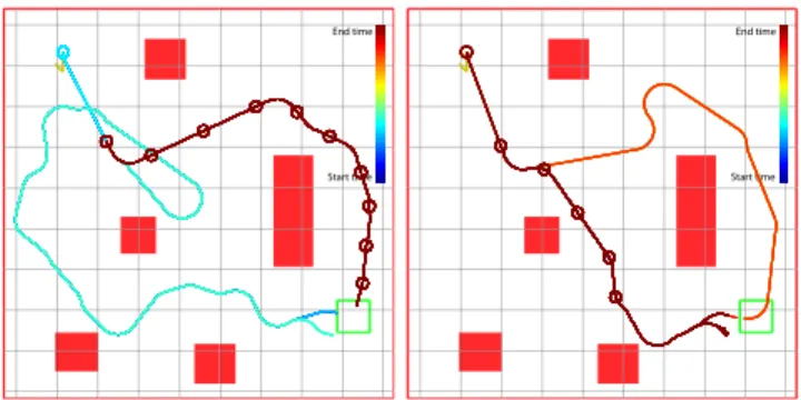
We conducted a series of tests with both the RRT∗anytime algorithm as well as the RRT-based planner. The vehicle operated in a 20 m by 20 m packed gravel environment consisting of five obstacles (Fig. 6). The task was to navigate from a starting position in one corner to a 1.6 m goal region in the opposite corner while avoiding the obstacles. We manually specified the location of the obstacles. In each experiment, planning started immediately prior to the controller tracking the committed trajectory.
Figure 6 presents the result of four different tests with the RRT∗ anytime motion planner. The plots depict the best trajectory as maintained by the RRT∗ at different points during the plan execution (false-colored by time). In the scenario represented in the upper left, the RRT∗ initially identifies a sub-optimal path that goes around an obstacle but, as the vehicle begins to execute the path, the planner correctly refines the solution to a shorter trajectory. As the vehicle proceeds along the committed trajectory, the planner continues to rewire the tree as evident in the improvements near the end of the execution when the paths more directly approach the goal.
Start time End time Start time End time Start time End time Start time End time
Fig. 6. Four runs of the anytime RRT∗on the robotic forklift. Starting in the upper left, the forklift was tasked with driving to the goal region while avoiding obstacles. The trajectories indicate the optimal path as estimated by the RRT∗at different points in time during the execution and are false-colored by time. Circles denote the initial position for each path.
Start time End time
Start time End time
Fig. 7. Plans generated by the anytime planner using the standard RRT.
For comparison, Fig. 7 presents the resulting paths for the anytime planner utilizing the standard RRT. In the scenario depicted on the left, the RRT initially finds a looping trajec-tory that goes wide to the left but, after moving a few meters, discovers a shorter path that takes the vehicle wide to the right. At this point, the structure of the tree biases the RRT toward refinements that improve the trajectory only locally. In the second test, the RRT revises the initial trajectory that unnecessarily goes to the right of the obstacle and discovers a shorter, yet sub-optimal path to the goal.
VI. CONCLUSION
Incremental sampling-based motion planners have been used successfully to plan trajectories for vehicles with re-stricted dynamics operating in the presence of obstacles. The appeal of incremental planners such as the RRT stems, in part, from their efficiency at identifying feasible motion plans and their intuitive implementation. However, the feasible solutions produced by the RRT tend to be far from optimal.
This paper described an anytime motion planning algo-rithm that uses the RRT∗ to solve for and improve solutions to the motion planning problem in an online fashion. We described methods that enable the planner to asymptotically converge to the optimal solution online, during trajectory execution. We used Monte Carlo simulation to evaluate convergence of the anytime RRT∗ algorithm, and compared it to a standard RRT-based motion planner. We further demonstrated the algorithm’s performance while planning trajectories for a large ground vehicle.
ACKNOWLEDGMENTS
We gratefully acknowledge the support of the U.S. Army Logistics Innovation Agency, the U.S. Army Combined Arms Support Command, and the Department of the Air Force (Air Force Contract FA8721-05-C-0002).
REFERENCES
[1] J. Latombe, “Motion planning: A journey of robots, molecules, digital actors, and other artifacts,” Int’l J. of Robotics Research, vol. 18, no. 11, pp. 1119–1128, 1999.
[2] A. Bhatia and E. Frazzoli, “Incremental search methods for reacha-bility analysis of continuous and hybrid systems,” in Hybrid Systems: Computation and Control, ser. Lecture Notes in Computer Science, R. Alur and G. Pappas, Eds., Mar. 2004, no. 2993, pp. 451–471. [3] M. S. Branicky, M. M. Curtis, J. Levine, and S. Morgan,
“Sampling-based planning, control, and verification of hybrid systems,” IEEE Proc. Control Theory and Applications, vol. 153, no. 5, pp. 575–590, Sept. 2006.
[4] Y. Liu and N. Badler, “Real-time reach planning for animated char-acters using hardware acceleration,” in IEEE Int’l Conf. on Computer Animation and Social Characters, 2003, pp. 86–93.
[5] J. Reif, “Complexity of the mover’s problem and generalizations,” in Proc. IEEE Symp. on Foundations of Computer Science, 1979. [6] L. Kavraki, P. Svestka, J. Latombe, and M. Overmars, “Probabilistic
roadmaps for path planning in high-dimensional configuration spaces,” IEEE Trans. on Robotics and Automation, vol. 12, no. 4, pp. 566–580, 1996.
[7] S. M. LaValle and J. J. Kuffner, “Randomized kinodynamic planning,” Int.’l J. of Robotics Research, vol. 20, no. 5, pp. 378–400, May 2001. [8] Y. Kuwata, J. Teo, G. Fiore, S. Karaman, E. Frazzoli, and J. How, “Real-time motion planning with applications to autonomous urban driving,” IEEE Trans. on Control Systems, vol. 17, no. 5, pp. 1105– 1118, 2009.
[9] S. Karaman and E. Frazzoli, “Incremental sampling-based algorithms for optimal motion planning,” in Proc. Robotics: Science and Systems (RSS), 2010.
[10] S. Thrun et al., “Stanley: The robot that won the DARPA Grand Challenge,” J. of Field Robotics, vol. 23, no. 9, pp. 661–692, Sept. 2006.
[11] S. Teller et al., “A voice-commandable robotic forklift working along-side humans in minimally-prepared outdoor environments,” in Proc. IEEE Int’l Conf. on Robotics and Automation (ICRA), May 2010. [12] A. Correa, M. R. Walter, L. Fletcher, J. Glass, S. Teller, and
R. Davis, “Multimodal interaction with an autonomous forklift,” in Proc. ACM/IEEE Int’l Conf. on Human-Robot Interaction (HRI), Mar. 2010.
[13] M. R. Walter, S. Karaman, E. Frazzoli, and S. Teller, “Closed-loop pallet engagement in an unstructured environment,” in Proc. IEEE/RSJ Int’l Conf. on Intelligent Robots and Systems (IROS), Oct. 2010. [14] S. Karaman and E. Frazzoli, “Optimal kinodynamic motion planning
using incremental sampling-based methods,” in Proc. IEEE Conf. on Decision and Control (CDC), Dec. 2010.
[15] M. Likhachev, D. Ferguson, G. Gordon, A. Stentz, and S. Thrun, “Anytime search in dynamic graphs,” J. Artificial Intelligence, vol. 172, pp. 1613–1643, Sept. 2008.
[16] L. Dubins, “On the curves of minimal length on average curvature, and with prescribed initial and terminal positions and tangents,” American J. of Mathematics, vol. 79, no. 3, pp. 497–516, 1957.