Analysis and modeling of induced seismicity in petroleum reservoirs

.1111 W I 11110 III11 1111 6 111 1 h i '1W II I I I 'LIh I I i 11 111 1 jiI ' I j II I

Analysis and Modeling of Induced Seismicity

in Petroleum Reservoirs

by

Heather J. Hooper

B.S., Earth, Atmospheric, and Planetary Sciences

Massachusetts Institute of Technology, 2000

Submitted to the Department of Earth, Atmospheric, and Planetary Sciences

in partial fulfillment of the requirements for the degree of

Professional Masters in Geosystems

at the

MASSACHUSETTS INSTITUTE OF TECHNOLOGY

September 2002

LINDGREN

©

Massachusetts Institute of Technology 2002.

All rights reserved.

NOV

2

62002

LIBRARIES

A uthor... ...

partment of Earth, Atmospheric, and Planetary Sciences

_ August 30, 2002

Certified

by ...

..

...

Dr. Daniel Bums

Research Scientist

Thesis Supervisor

Accepted

by ... ... ...

Dr. Ronald G. Prinn

Head, Department of Earth, Atmospheric, and Planetary Sciences

Analysis and Modeling of Induced Seismicity

in Petroleum Reservoirs

by

Heather J. Hooper

Submitted to the Department of Earth, Atmospheric, and Planetary Sciences on August 30, 2002, in partial fulfillment of

the requirements for the degree of Professional Master in Geosystems

Abstract

Since 1998, a producing oil field in Oman has been experiencing

microearthquake activity. The aim of this project is to compare numerical models of wave propagation using simple source representations to a small subset of these microearthquakes, with three goals in mind: 1) to understand whether the microearthquakes are generated by movement along a known fault system in the field, or by some other mechanism; 2) if the source is fault related, to better understand what kind of movement is occurring on the fault; and 3) to see if this simple modeling method provides useful results, and forms a basis for

future work. Synthetic waveforms are generated using a one-dimensional,

discrete wavenumber numerical model (Bouchon, 1980) with two simple source representations: an explosive point source and a vertical force. Comparison of the synthetic waveforms to the microearthquake data indicates that the vertical force results in a better match than the explosive point source. In addition, a simple model consisting of the superposition of four vertical forces (representing vertical fault rupture), results in waveforms that are very similar to the recorded events. These results suggest that the source of the microearthquakes is motion along a near-vertical normal fault system that has been mapped in the field. These results are also consistent with work by Sze and Toksoz (2001) in which relocation of the same events imaged a near-vertical normal fault in the field. Further work using fault rupture source modeling may provide additional insight into the amount of fault motion that is occurring in relation to these events.

Thesis Supervisor: Dr. Daniel Burns Title: Research Scientist

Acknowledgments

I would like to thank my thesis advisor, Dr. Dan Bums, for his patience and guidance, and for his advice

throughout the year. I would also like to thank Professor Dale Morgan for his understanding and his humor. Thanks to Dr. Edmond Sze, whose results were the basis for this project, and who answered innumerable emails, to Dr. Michel Bouchon, who wrote the code, and to Dr. Sadi Kuleli who has been invaluable. Thanks also to Amro Farid, who devoted hours to helping me understand signal processing. Lastly, I would like to thank Justin Przedwojewski, for his help, support, and encouragement over the past year, and for so many other things.

' 40II iii , I

Contents

1 Introduction ...

13

1.1 O utline ...

14

2 Background Information...15

2.1 Microearthquakes in Petroleum Production... 15

2.2 Description and History of Yibal Oilfield ... 15

3 Microearthquake Data...

...

19

3.1 Data Provenance and Description ...

19

3.2 Data Processing ...

23

4 Methodology...25

4.1 The Method ...

25

4.2 The Discrete Wavenumber Program ... 26

4.3 The Velocity Model ...

29

4.4 Sze and Toksoz's P and S Picks ... ..

29

5 Results and Discussion...

...

33

5.1 Particle Motion Analysis of Microearthquake Data ...

33

5.2 Analysis of Model Output ... ... 37

5.3 Comparison of Microearthquake Data and Model Output ... 40

5.4 An Experiment With Fault Rupture ... 47

6 Conclusions and Further Work ... 51

References...53

Appendices

A: Receiver Information...55

B: Microearthquake Information...56

C: Preliminary Processing of Microearthquake Data... 57

D: Particle Motion Analysis for Determination of Backazimuth ... 62

E: Periodicity Length...64

F: Particle Motion Analysis of Model Output...

...

67

G: Sze and Toksoz's Picks, Vertical Force Model Output Arrivals, and

Percentage Differences...

71

List of Figures

2-1 Mohr Diagram Demonstrating the Effect of Pore Fluid Pressure on the Fracture

Stability of Rock. (Twiss and Moores, 1992)...

... 16

2-2

Map of the Oman Region Showing Structural Elements and Major Oil and Gas

Fields. (Sze and Toksoz, 2001)... 17

3-1 Sample Waveforms Collected by the Yibal Oil Field Passive Seismic

M onitoring System ...

20

3-2 2-D Plot of Locations of All Recorded Events in Yibal Oil Field up to July 13,

2000. (Yibal Natih Compaction Monitoring Project Interim Report, 2001)...21

3-3 Locations of Seismic Monitoring Wells and Microearthquakes ... 21

3-4 a,b Microearthquake Depths Plotted Against Latitude and Longitude ... 22

3-5 Frequency Content of Displacement Waveform for Event 38, Receiver VA11...24

4-1 Explosive Point Source in a Homogeneous Halfspace ... 27

4-2 Vertical Force in a Homogeneous Halfspace ... 27

4-3 Original Velocity Model Developed by Petroleum Development Oman ... 30

4-4 Changed Velocity Model Used for This Project ... 30

4-5 Sample Waveform Created Using Original Velocity Model and Vertical Force...31

4-6 Sample Waveform Created Using Changed Velocity Model and Vertical Force...31

5-1 Particle Motion Analysis of Microearthquake Data

-

Radial vs. Transverse

-

P-wave...33

5-2 Particle Motion Analysis of Microearthquake Data

-

Radial vs. Transverse

-

S-wave...34

5-3 Particle Motion Analysis of Microearthquake Data

-

Radial vs. Transverse

-

Other

Energy

-

Possible Surface W ave? ...

34

5-4 a,b Microearthquake Data from Event 38, Receiver VA 11, With Arrivals Marked,

Vertical and Radial Components...

35, 36

List of Figures, continued

5-5

a,b Model Output Using Explosive Point Source, Vertical and Radial Components...37, 38

5-6

a,b Model Output Using Vertical Force, Vertical and Radial Components ...

...

39

5-7

a,b Comparison Between Microearthquake Data and Explosive Point Source

M odel O utput...

41, 42

5-8

a,b Comparison Between Microearthquake Data and Vertical Force Model Output...43, 44

5-9 Results of Fault Rupture Experiment Using Four Vertical Point Sources and

Original Velocity Model, Vertical Component... ... 48

5-10 A Single Vertical Force Model Output, Vertical Component ... 49

C-1 Displacement Waveforms Obtained by Integrating Velocity Waveforms

-

No

Corrections Made ... ...

...

57

C-2 Displacement Waveforms after Subtraction of Trendlines ... 58

C-3 Displacement Waveforms After Removal of Running Average... 59

C-4 Displacement Waveforms After Rotation of Horizontal Components to True

N orth and E ast...60

C-5 Corrected and Rotated Displacement Waveforms Resulting from Processing of

O riginal V elocity D ata...

... 61

D-1 Particle Motion Analysis Determination of Backazimuth ... 63

E-1 Periodicity Length = 5,000m ... ... . .. 64

E-2 Periodicity Length

10,000m ... ... 65

E-3 Periodicity Length = 20,000m ... ...

65

E-4 Periodicity Length = 30,000m ...

... ...

... 66

List of Figures, continued

Particle Motion Plot

Particle Motion Plot

Particle Motion Plot

Particle Motion Plot

Particle Motion Plot

for Explosive Point Source S-Wave ... 68

for Vertical Force P-Wave ... 69

for Vertical Force S-Wave...

... 69

for Vertical Force Downward P-Wave After S-wave ... 70

for Vertical Force Energy After Downward P-Wave ... 70

F-2

F-3

F-4

F-5

F-6

List of Tables

5-1 Average Percentage Difference Between Edmond Sze and Toksoz's Picks and

Vertical Force Model Output Arrival Times for All Events, All Receivers

(Using Changed Velocity Model) ...

46

A-i Receiver Locations and Other Information ... 55

B-1 Pertinent Information on Microearthquakes ... 56

D-1 Results of Particle Motion Analysis for Event 38 ...

63

Chapter 1

Introduction

Induced seismicity refers to earthquakes that are caused, directly or indirectly, by human activities, such as oil and gas production, mining, waste disposal, dam construction, and geothermal energy production. These activities often cause changes in the local stress field, which can result in both aseismic and seismic deformation. Induced earthquakes are usually small in magnitude (<4) and are

therefore referred to as microearthquakes, however larger earthquakes with magnitudes between 5 and 7

have also been attributed to human activities'-'.

The analysis of induced microearthquakes can be helpful in understanding the effects of oil and gas production in petroleum reservoirs and surrounding regions. Microearthquake data can be used to delineate faults and other geologic structures within and surrounding a petroleum reservoir, to gain a better understanding of the state of stress in the reservoir, to monitor the effects of compaction and subsidence, to understand the potential for damage to oil and gas bearing formations, production equipment, and the environment, and to help production companies plan for the future. The potential occurrence of large earthquakes, and the resulting destruction of property and potential for injury, is obviously also a serious concern. Unfortunately the likelihood of a large earthquake occurring in a given oilfield is unknown, however monitoring of microearthquakes can be helpful in understanding potential seismic hazard.

The Yibal Oil Field in Oman has been experiencing compaction and subsidence for several years, and potentially severe damage to formations, equipment and the environment is predicted. Currently, a detailed compaction monitoring project is underway at Yibal Oil Field, involving everything from finite element modeling to radioactive marking of formations and downhole casing to passive seismic

monitoring.12

1' Nicholson and Wesson, 1992; McGarr, 1991.

1-2 Yibal Natih Compaction Monitoring Project Interim Report, January 2001

Microseismicity monitoring was begun at Yibal Oil Field in 1999 in order to better understand microearthquake activity occurring in the field. Knowledge of the distribution, geometry and movement of faults in and around the oil field is useful in planning future development and remediation. This project is part of that effort.

Over 500 microearthquakes have been recorded at Yibal since October, 1999. Previous work by Sze and Toksoz (2001), of the Earth Resources Laboratory at MIT, used some of these microearthquakes to image a fault in the oil field. Building on Sze and Toksoz's work, and using a computer program developed by Michel Bouchon, we create synthetic waveforms that resemble the actual microearthquake waveforms, then compare the two. This approach allows us to confirm whether the microearthquakes are associated with the fault, or with other processes such as pore collapse. It also allows us to better understand what kind of movement is occurring on the fault. It also shows that this method is viable for microearthquakes in Yibal Oil Field, and forms a basis for future work.

1.1 Outline

Chapter 2 provides background information on the project, including a summary of the relationship between microearthquakes and petroleum production, and a description of the geology and history of Yibal Oilfield. Chapter 3 deals with the acquisition and processing of the microearthquake data. It also includes a brief summary of Sze and Toksoz's (2001) previous work on the project. Chapter 4 discusses the methodology for the project, as well as the program used to create the synthetic data. Chapter 5 presents the results of the project. Chapter 6 presents conclusions, as well as suggestions for future work.

Chapter 2

Background Information

2.1 Microearthquakes in Petroleum Production

Much research has been performed on the relationship between microearthquakes and petroleum production. In oil and gas fields, induced seismicity is thought to represent shear failure on planes of weakness, including pre-existing faults, and is caused by changes in the local state of stress. These changes can be caused by two mechanisms: fluid pressure reduction through oil and gas extraction, and

fluid pressure increase through injection of fluids2-1. For the case of fluid extraction in particular, McGarr

(1991) found that the removal of large volumes of fluid causes stress changes associated with subsidence

and unloading effects. Pennington et al. (1986) have suggested that fluid extraction may cause

aseismically slipping faults to lock up, which can eventually result in a seismic stress release. Injection of fluids increases the pore fluid pressure of the rocks, resulting in a reduction of the effective stress. This reduction of effective stress lowers the strength of the rocks, which can lead to failure, either by

fracturing, or by slip along pre-existing faults2 2 (Figure 2-1). In addition, it has been suggested that

injection of fluids near or into an inactive fault zone may lubricate the fault, leading to re-activation.

2.2 Description and History of the Yibal Oil Field

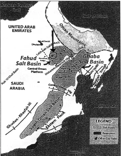
The Yibal Oil Field is located in the Fahud Salt Basin in north-central Oman (Figure 2-2).

Currently there are two producing formations at Yibal: the Natih gas reservoir and the Shuaiba oil reservoir beneath it. Both consist of heavily folded and faulted Cretaceous limestones. The reservoir is

intersected by regional normal faults with strike approximately SE-NW and SW-NE .23

2-1 _{Grasso et al, 1992}

2-2 Twiss and Moores, 1992, pp. 177-178, 194

2-3 Sze and Toksoz, 2001

Yibal was discovered in 1962, and has been in constant production since at least 1978. It is Oman's largest producing oil field, and is an important component of Oman's energy strategy. Oil and gas production at Yibal must continue until at least 2005 in order to maintain the domestic energy supply24.

Figure 2-1 Mohr Diagram Demonstrating the Effect of Pore Fluid Pressure on the Fracture Stability of Rock. Effective normal stress is plotted on the x-axis, and shear stress is plotted on the y-axis. A. At small differential stress, an increase in pore fluid pressure leads to tension fracture. B. At large differential stress, an increase in pore fluid pressure leads to shear fracture. (Twiss and Moores, 1992)

The Yibal Oil Field has been experiencing compaction and subsidence for several years, resulting

in over 50 cm of subsidence over the center of the field. Although there is currently no reported damage

to wells, continuing compaction may have potentially serious financial consequences. Obtaining a better understanding of the processes acting in the field is therefore of prime importance.

2-4 _{Yibal Natih Compaction Monitoring Project Interim Report, January 2001}

20,- 18W

Most of the subsidence at Yibal is attributed to compaction of the Natih gas formation, where strains of approximately 1.5% have already been measured. This formation may develop much larger

strains as reservoir pressure declines over the next few years.2-5 _{There is a possibility that compaction}

may also be occurring in deeper formations. Microearthquakes have occurred throughout the central portion of the reservoir, most of them located at depths below both the Natih and Shuaiba formations. Several possible sources have been posited for the microearthquakes: fluid flow within the reservoir, pore

collapse, and fracturing / slip on faults. In the case of the deeper events, the last possibility is the most

likely. As mentioned in Section 2.1, increased pore pressure can lead to fracturing or slip on pre-existing faults. At the Yibal Oil Field, large volumes of water are re-injected into the Shuaiba reservoir on a daily basis. This re-injection could be raising the pore fluid pressure high enough to cause slippage along existing fault planes.

Figure 2-2 Map of the Oman Region Showing Structural Elements and Major Oil and Gas Fields. (Sze and Toksoz, 2001)

Microearthquakes were first reported by staff at Yibal oil field in 1998. In 1999 a passive seismic monitoring system was installed. 239 seismic events were logged in the first year of operation, most with magnitude <1. (Microearthquake occurrences at other oil/gas fields reported in the literature have ranged from 78 per year at a gas field in France2 -6 to almost 1900 per year in Clinton County, Kentucky2-7.) The largest event at Yibal was reported with a local magnitude of 2.24. Depths of the events are between I and 5 km below the surface.

2-6 Feignier and Grasso, 1990 2-7 Rutledge _{et al, 1998}

ANIE l i i I IpjIIh,

Chapter 3

Microearthquake Data

3.1 Data Provenance and Description

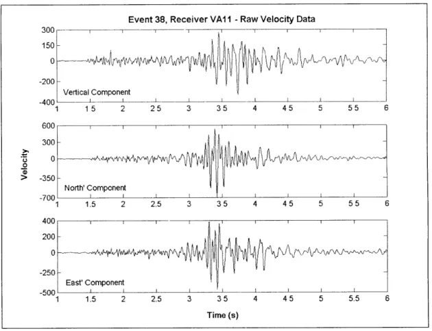
The passive seismic monitoring system at Yibal Oil Field has been operational since November of 1999. The system consists of five shallow monitoring wells designated VAl through VA5. Each monitoring well contains four 3-component, 4.5Hz geophones at depths of 135m, 140m, 145m, and 150m.3-1 Locations and other pertinent receiver information are listed in Appendix A. The 3-component geophones consist of one vertical component and two orthogonal horizontal components, designated North' and East'. Because of the difficulty inherent in installing downhole geophones, the horizontal components are at varying known azimuths from North and East. Data are sampled at a rate of 125 samples/s. Figure 3-1 shows sample waveforms.

Sze and Toksoz (2001) used microearthquake data from Yibal Oil Field to image a fault structure in the field. Microearthquakes recorded at Yibal Oil Field are located by Petroleum Development Oman using a single-station location method. Sze and Toksoz relocated a group of fourteen microearthquakes using two other methods: Hypoinverse 2000 and double difference. This group of microearthquakes was selected from the forty-four events recorded at Yibal during October, 2000, on the basis of similarity of initial location and waveform shape. Upon relocation using double difference, it became clear that ten of

these events were aligned along a structure that strikes NE-SW and dips at about 800 to the southeast.3 2

This is consistent with known faults in the area (Figure 3-2). Sze and Toksoz's conclusion was that these microearthquakes originated from slip on a fault, and that his revised locations effectively imaged the

fault plane.3 3

3-1 _{The microearthquake data used in this project was collected during October, 2000, at which time only data from}

the geophones located at depths of 150m was available. The geophones at depths of 150m are designated by the

number 1. For example, the 150m geophone in borehole VA 1 is designated receiver VA 11.

3-2 Sze, personal communication, 2002

3-3 _{Sze and Toksoz, 2001}

1 1.5 2 2.5 3 35 4 45 5 5.5 6 Time (s)

Figure 3-1 Sample Waveforms Collected by the Yibal Oil Field Passive Seismic Monitoring

System. These waveforms are from Event 38, the largest event used in this project, with

mL = 0.05.

This project seeks to confirm that these microearthquakes are due to slip on a fault, and to gain a preliminary understanding of motion on that fault, using nine of Sze and Toksoz's microearthquakcs. (One of the ten microearthquakes was substantially shallower than the other nine, and was excluded.) The locations used in this project are Sze and Toksoz's (2001) double difference locations. Figure 3-3 shows the locations of the microearthquakes, as well as the locations of the five wells of the seismic monitoring system. Figures 3-4a and 3-4b show depths of the events plotted against latitude and longitude. The magnitudes of the microearthquakes range between -0.88 and 0.05 on the local magnitude scale. Pertinent attributes of the events are listed in Appendix B.

Event 38, Receiver VA11 I - Raw Velocity Data

300 --- -- -150 -200 Vertical Component -400 -I I I 1 15 2 25 3 35 4 45 5 55 6 600 300 o 0 > R

-Tremor Locations

Figure 8. 2D Plot of Location of Tremors to 13-July-2000

Figure 3-2 2-D Plot of Locations of All Recorded Events in Yibal Oil Field up to July 13, 2000. Also shows major faults in the area. Note the two large normal faults extending across the field. Most of the microearthquake activity is located around or between these faults. (Yibal Natih Compaction Monitoring Project Interim Report, 2001)

Event and Station Locations

22.2 22.19 22.18 VA3 22.17 22.16 22.15 22.14 22.13 22.12 A Events A Event 38 O Stations VA4 VA5 VA5 IA VA2 VA1 55.97 55.98 55.99 56 56.01 56.02 56.03 56.04 56.05 56.06 Longitude (degrees)

Figure 3-3 Locations of Seismic Monitoring Wells and Microearthquakes ~~

- -~--1.- I I II

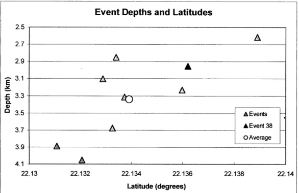
----Figure 3-4a Microearthquake Depths Plotted Against Latitude

Figure 3-4b Microearthquake Depths Plotted Against Longitude

Event Depths and Latitudes

A

3.

A

Event Depths and Longitudes

2.5

A

A

A

A

-3.2 Data Processing

The microearthquake data required some processing to allow for comparison with the numerical modeling results. The data were processed using a digital seismic signal-processing program called

PITSA (Programmable Interactive Toolbox for Seismological Analysis), written by Frank Scherbaum and

James Johnson, and freely available on the web.3-4 _{Each waveform was processed as follows:}

1. Numerical integration using Tick's Rule to convert velocity measurements to displacement

waveforms.

2. Baseline correction 1: Subtraction of Trendline. A trendline is calculated for each waveform using linear regression. This trendline is then subtracted from the waveform to remove any downwards trend in the data.

3. Baseline Correction 2: Removal of Running Average. A running average is removed from the data in order to remove low frequency artifacts.

4. Rotation of North' and East' horizontal components to true North and East.

5. Rotation of North and East horizontal components to radial and transverse components.

Appendix D contains figures demonstrating each step of the processing, as well as more detailed information on each processing step.

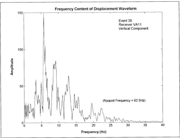
Note that deconvolution of the receiver response from the data was not performed. The

frequency content of the microearthquake displacement data is shown in Figure 3-5. The main

frequencies are all above 4.5Hz. Since the receiver response function for the geophones used at Yibal Oil Field is basically flat above 4.5Hz, deconvolution of the receiver response was deemed unnecessary.

3-4 http://lbutler.geo.uni-potsdam.de/service.htm

Frequency Content of Displacement Waveform

0 5 10 15 20 25 30 35 40

Frequency (Hz)

Figure 3-5 Frequency Content of Displacement Waveform for Event 38, Receiver VA11, Vertical

Component. Frequencies below 2Hz have been filtered out, since they are simply artifacts of the integration.

'ii-1 IYI_ __ __

Chapter 4

Methodology

4.1 The Method

The goal of this project is to learn more about the nature of the microearthquake sources, as well as movement on the fault. In order to do so, we create synthetic waveforms that resemble the actual microearthquake waveforms, then compare the two. The simplicity of the velocity model available for the region, the small number of seismic monitoring stations, the magnitude of the events involved, and the simplicity of the available source representations make it impossible to exactly duplicate the microearthquake waveforms with synthetic data. Instead, our aim is to do some initial modeling of the events. Three comparisons are made between the synthetic data and the microearthquake data:

* Travel times of the P and S waves,

* Relative amplitudes of the P and S arrivals, and * The overall appearance of the waveforms.

The modeling program contains two theoretical source representations. The comparisons listed above allow us to judge which of the two source representations produces synthetic data closest to the microearthquake data, and therefore which of the theoretical sources is closest to the actual source mechanism. This approach allows us to confirm whether the microearthquakes are associated with faulting (specifically the fault imaged by Sze and Toksoz (2001)) or with other processes such as pore collapse. It also allows us to understand more about the movement occurring on the fault, which is important for future planning of production in the Yibal Oil Field. In addition, a good match between synthetic data and microearthquake data shows that the method is viable, and forms a basis for future work.

4.2 The Discrete Wavenumber Program

One way of calculating synthetic seismograms is to represent the wave field emitted by the source as plane waves propagating at a practically infinite number of angles. (This translates into a practically infinite number of horizontal wavenumbers.) Calculation of displacement, stress, etc., requires summing this large number of plane waves by integrating over the horizontal wavenumber. In general, this integral

is solved numerically, requiring intensive computation.

The discrete wavenumber method is based on an exact discretization of the wave field emitted by the source. This is accomplished by replacing the single source with an infinite periodic array of sources. This source array results in a representation of the wave field as a superposition of plane waves, and because of wave interference, the waves only propagate at discrete angles. (This is similar in principle to the diffraction of light by a grating.) The result is a simplification of the wavenumber integral to a summation, which is much quicker and less costly to compute. Important parameters of the program are discussed in the following sections.

The discrete wavenumber program used to create the synthetic data was developed by Michel Bouchon, of Universit6 Joseph Fourier - Grenoble. It utilizes the discrete wavenumber method of Bouchon and Aki4-1 and Kennett's method of reflectivity and transmissivity matrices4-2

4.2.1 Sources

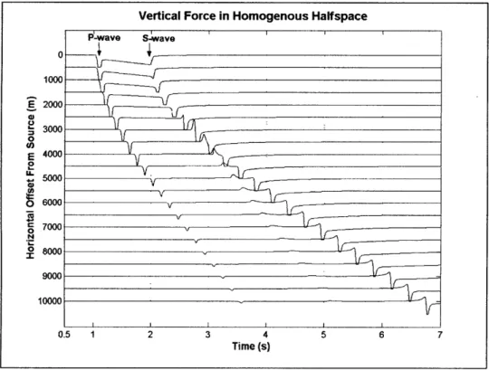
There are two theoretical source representations available for use with the program: an explosive point source and a vertical force. The explosive point source represents source mechanisms such as pore collapse, whereas the vertical force is a simple representation of fault motion. Figures 4-1 and 4-2 demonstrate the effects of the two sources in a homogeneous halfspace. Note that the explosive source (Figure 4-1) emits only P-waves, while the vertical force (Figure 4-2) emits both P- and S-waves.

4-1 Bouchon and Aki, 1977

Explosive Point Source in Homogenous Halfspace

Figure 4-1 Explosive Point Source in a Homogenous Halfspace. Vertical receiver.

Vp = 3000m/s, Vs = 1563m/s. Source depth = 3000m.

Figure 4-2 Vertical Force in a Homogenous Halfspace. Vertical

Vp = 3000m/s, Vs = 1563m/s. Source depth = 3000m.

receiver.

Time (s)

Vertical Force in Homogenous Halfspace

P-wave S-wave 0 1000 E 2000 3000 E 4000 0 S5000 V 6000 7000 o 8000 I Time (s) iiYI r

4.2.2 Receivers

In this version of the program, the wavenumber discretization is done in one dimension, which

restricts the program to two-dimensional wave propagation problems.4-3 For this reason, there are only

two receiver components available in the program: vertical and radial.

4.2.3 Number of Time Samples, Length of Time Window

For this project, the number of time samples (1024) and the length of the time window (8.192s) are chosen in order to duplicate the sampling frequency of the microearthquake data, which is 125 samples / second.

4.2.4 Periodicity Length

The length of the interval between the sources in the periodic array is chosen by the user, and depends on the desired time window of the modeling. The distance between sources must be large enough that energy emitted by the fictitious sources doesn't reach the receiver during the time window of interest. Energy from the fictitious sources is also attenuated slightly by the addition of a small imaginary part to the frequency during the summation. A periodicity length of 80,000m was chosen for this project. See Appendix E for figures demonstrating the effect of changes to the periodicity length.

4.2.5 Central Period of Ricker Wave

The pressure / force pulse emitted by the source is a Ricker wavelet, and the central period of that pulse can be changed by the user. Through experimentation, a value of 0.04s was chosen in order to match the frequency content of the microearthquake data as closely as possible.

4.2.6 Free Surface Effects

The user can choose to turn free surface effects (surface reflections, surface waves, and ground roll) on or off. There was some question as to whether it was appropriate to include free surface effects, since the receivers are at a depth of 150m below the surface, however after some experimentation, it was decided to turn free surface effects on for this project.

4-3 Bouchon has published several papers presenting extensions of the method to three dimensions: Bouchon, 1979

4.2.7 Dispersion / Anelastic Attenuation

Q values for the rocks present in the Yibal Oil Field are estimated to be between 40 and 100.

Numerical modeling was tried using several different values of Qp and Qs, however the only effects were

a slight decrease in the amplitude of the displacement and some smoothing of the waveforms. Qp and Qs

values were therefore set to 10,000, resulting in negligible anelastic attenuation.

4.3 The Velocity Model

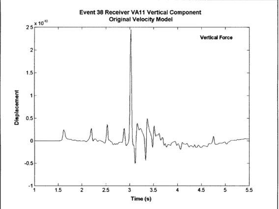
The original velocity model for Yibal Oil Field was developed by Petroleum Development Oman (Figure 4-3). The synthetic waveforms created using the original velocity model are very simple, and their general character is not a good match for the microearthquake data. In order to try to achieve a better fit with the character of the microearthquake data, we tested the effect of altering the velocities of the top two layers. A lower velocity near-surface layer results in more reflections in the layer, creating a more complicated output that is closer in character to the microearthquake data. Figure 4-3 shows the original velocity model, and Figure 4-4 shows the changed velocity model. Figures 4-5 and 4-6 show sample waveforms created using the original and changed velocity models. We generate model output using both of these velocity models. (Note: since the deepest microearthquake is 4,05 1m, Figures 4-3 and 4-4 only show the velocity model down to a depth of 4,500m.) For both models, the ratio between the S and P velocities is 1.92. Densities for the models were assumed to start at 2.0g/cc in the near-surface layer and increase by 0.1 g/cc per layer.

4.4 P and S Picks

Sze and Toksoz (2001) picked P and S arrival times for the microearthquake data. The low signal to noise ratio of the data made it difficult to do so by traditional methods, so he used two analytical

methods to aid in picking the correct arrival times: polarization and three-component amplitude.4-4 _His

picks are used in the travel time comparisons between the model output and the microearthquake data.

Original Velocity Model

Figure 4-3 Original Velocity Model Developed by Petroleum Development Oman

Changed Velocity Model

0-500 1000 1500 E 2000 o 2500 3000 3500 - . 4000 4500 500 1000 1500

Figure 4-4 Changed Velocity

2000 2500 3000 3500 4000 4500 5000

Layer Velocity (m/s)

Model Used For This Project

1000 1500 2000 2500 3000 3500

Layer Velocity (m/s)

Event 38 Receiver VA11 Vertical Component Original Velocity Model

x 101"0

4.5 5 5.5

1.5 2 2.5 3 3.5

Time (s)

Figure 4-5 Sample Waveform Created Using Original Velocity Model and Vertical Force

Event 38 Receiver VA1 I Vertical Component

x 101 Changed Velocity Model

2.5 Vertical Force 2 1.5

1

Figure 4-6 Sample Waveform Created Using Changed Velocity Model and Vertical Force

1 1 11 Ih 1, 1 1111'' 11111111111 W 1II111IN I III I I IlY

Chapter 5

Results and Discussion

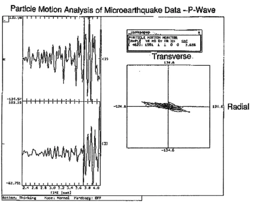
5.1 Particle Motion Analysis of Microearthquake Data

Particle motion analysis of the microearthquake data was performed to establish which arrivals

are present in the data. Figures 5-1 to 5-3 demonstrate the particle motion analysis, and Figures 5-4a and

5-4b show an example of the microearthquake data with the arrivals labeled.

Particle Motion

Analysis of Microearthquake Data --P-Wave

Radial

Figure 5-1 Particle Motion Analysis of Microearthquake Data - Radial vs. Transverse - P-wave

Particle Motion Analysis of Microearthquake Data

-

S-Wave

1

TransvemS

baor: Thirklrg Mod :bro±eal -G O, OFF

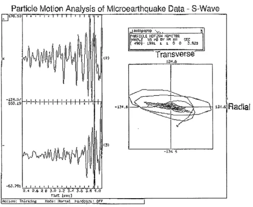
Figure 5-2 Particle Motion Analysis of Microearthquake Data - Radial

vs. Transverse - S-wave (The P-wave trace is also shown in this figure) Particle Motion Analysis of Microearthquake Data -Surface Wave?

Figure 5-3 Particle Motion Analysis of Microearthquake Data - Radial vs. Transverse - Other Energy - Possible Surface Wave?

r

Radial

Radial

"iL , -I # I I I |I I I I I I- I I I l I

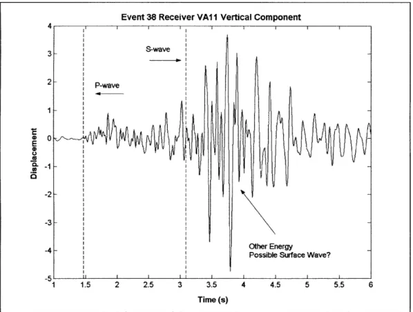
Event 38 Receiver VAI I Vertical Component 4 4 I I I I I I 3 S-wave 311 0 -2 -3-4 Other Energy

Possible Surface Wave?

-5_{5II I I I I I I I}

1 1.5 2 2.5 3 3.5 4 4.5 5 5.5 6

Time (s)

Figure 5-4a Microearthquake Data from Event 38, Receiver VAl1, Vertical Component, With Arrivals Marked. Dashed Lines denote Picks for P and S Arrivals from Sze and Toksoz (2001).

The particle motion plots in Figures 5-1 and 5-2 clearly identify the P- and S-waves, and the arrival times of both P and S coincide well with Sze and Toksoz's picks. The nature of the largest wave

packet (marked "Other Energy -Possible Surface Wave?" in Figures 5-4a and 5-4b) is uncertain. This

wave packet seems at first glance to be a surface wave, however several factors make that interpretation unlikely:

* Surface waves are generally dispersive, and there is very little dispersion present in the wave packet

* The particle motion analysis of this portion of the waveform is inconclusive. Surface waves generally plot as large elliptical traces in radial-transverse particle motion space. The trace plotted in Figure 5-3 is very small for a surface wave. In addition, watching the trace as it progresses in time gives one a sense of random motion, rather than the more organized motion expected of a surface wave

* Since surface wave amplitude decreases quickly with depth below the surface, the depth of the receivers (150m below the surface of the ground) suggests that any surface wave arrivals would have reduced amplitudes.

III-* The model output, which in theory should be similar to the microearthquake data, contains little to no surface wave energy.

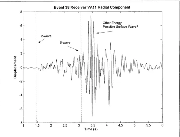
Event 38 Receiver VAI i Radial Component

Other Energy

6 Possible Surface Wave?

P-wave 4 I 4 S-wave 2- -2--4 -6 -8 1 1.5 2 2.5 3 3.5 4 4.5 5 5.5 6 Time (s)

Figure 5-4b Microearthquake Data from Event 38, Receiver VAl1, Radial Component, With

Arrivals Marked. Dashed Lines denote Picks for P and S Arrivals from Sze and Toksoz (2001).

Although it is difficult to be certain, it is more likely that this wave packet consists of a collection of multiply reflected, refracted and scattered energy - basically contaminated P- and S-waves - rather than surface wave arrivals. It is possible, however, that a small amount of the energy in this wave packet is surface wave energy.

ii IIm 10 OMNIII1 i dl.l ..lilII .. IId$k,

5.2 Analysis of Model Output

Identification of the arrivals in the model output was accomplished through a combination of

visual inspection, approximate calculations of travel times5-', and particle motion analysis of the model

output. (Examples of the particle motion analysis for each major type of arrival can be found in Appendix F.)

5.2.1 Explosive Point Source

Figures 5-5a and 5-5b show the vertical and radial components of the model output for Event 38, Receiver VAl 1, created using an explosive point source. Model output for other events and receivers is

similar. Arrivals are labeled on the figures.

S10. Explosive Source - 38VA11 I Vertical Component

P-wave reflected 0.5 off surface 0 -0 _-1 5₀ P-wave -1.5 1.5 2 2.5 3 3.5 Time (s)

Figure 5-5a Model Output Using Explosive Point Source. Event 38, Receiver VA 1, Vertical Component. Changed Velocity Model.

5-1 Approximate calculations of travel times were performed by dividing the approximate distance traveled through

Figure 5-5b Model Output Using Explosive Point Source. Event 38, Receiver VAIl, Radial

Component. Changed Velocity Model.

Although the explosive point source emits only P-waves (see Section 4.2.1), conversion to Sv-waves occurs at layer boundaries, resulting in some S-wave arrivals at the receiver.

5.2.2 Vertical Force

Figures 5-6a and 5-6b show the vertical and radial components of the model output for Event 38,

Receiver VA 1, created using the vertical force as the source. Model output for other events and

receivers is similar. Arrivals are labeled on the figures.

Note that the model output for the vertical force is much more complicated than the model output for the explosive point source. This is likely to make it a better match to the microearthquake data (see Section 5.3). Note the small "other reflections..." packet in the vertical force model output. Although it isn't nearly as large as the "other energy" packet in the microearthquake data, it is likely similar in nature. Its lower amplitude is likely due to the small number of layers in the theoretical velocity model, which reduces the capacity of the model to replicate scattering, as well as multiple reflections and refractions.

Vertical Force - 38VA11 I Vertical Component

Time (s)

Figure 5-6a Model Output Using Vertical Force. Event 38, Receiver VAl1, Vertical Component. Changed Velocity Model.

Figure 5-6b Model Output Using Vertical Force. Event 38, Receiver VAl1, Radial Component. Changed Velocity Model.

x 10'0

2.5

5.3 Comparison of Microearthquake Data and Model Output

As mentioned in Section 4.1, it is impossible to exactly duplicate the microearthquake waveforms using the synthetic data. Instead, our aim is to do some initial modeling of the events. Three comparisons are made between the synthetic data and the microearthquake data:

1. Arrival times of the P and S waves,

2. Relative amplitudes of the P and S arrivals, and 3. The overall appearance of the waveforms

Note that output arrival times generated by the model contain a systematic time shift relative to the microearthquake data. The receivers in the seismic monitoring system at Yibal Oil Field are located 150m below the surface of the ground, however the discrete wavenumber code only allows the user to place receivers at the surface. The result is that waves in the model pass through an extra 150m (or more) of ground before reaching the receiver. We made several attempts to make up for this difference by altering layer depths, changing the depths of the events, etc. Every attempt resulted in serious problems with the model output, so we decided to simply note the extra distance traveled and take it into account in our comparisons. The extra distance results in an extra 0.09 seconds of travel time for P waves, and an extra 0.17 seconds of travel time for S waves (approximately). These errors are fairly small, considering the other simplifications inherent in the modeling and method, however they should be kept in mind when

evaluating arrival time comparisons.

5.3.1 Comparison of Explosive Point Source Model Output and Microearthquake Data

Figures 5-7a and 5-7b show a comparison between the microearthquake data and the explosive point source model output. The data and model output shown in these figures are for Event 38, Receiver

VA11.

Arrival times of P and S waves: The match between the explosive point source model

output and the microearthquake data is generally fairly good, particularly for, the S-waves. For example, although the P arrival in Figure 5-7b is a little late, the S arrival coincides exactly with Sze and Toksoz's pick.

Comparison - Explosive Source - 38VA11 - Vertical

Figure 5-7a Comparison Between Microearthquake Data and Explosive Point Source Model

Output for Event 38, Receiver VAl1, Vertical Component. Microearthquake data is in

turquoise, model output is in black. Red lines are picks for P and S arrivals from Sze and Toksoz (2001). Model output was created using the changed velocity model.

Relative amplitudes of the P and S arrivals: In the microearthquake data, the P amplitude is much smaller than the S amplitude. In the explosive point source model output, the P amplitude is up to 2 times larger than the S amplitude. (In Figure 5-7b, the P arrival's

amplitude is approximately 7.6, while the S arrival's amplitude is approximately 5.2.) In this

respect, the model output and the microearthquake data do not match well.

Overall appearance of the waveforms: The appearance of the model output is not even

close to the appearance of the microearthquake data. For both the vertical and radial components, the microearthquake data progresses from a low-amplitude P arrival, to a slightly higher-amplitude S arrival, and finally to a broad packet of high-amplitude energy, which peaks and then gradually decreases to lower amplitudes.

E E o .=L-1 aa 0 1 1.5 2 2.5 3 Time (s)

_ _

Comparison - Explosive Source - 38VA11 - Radial

Figure 5-7b Comparison Between Microearthquake Data and Explosive Point Source Model Output for Event 38, Receiver VA11, Radial Component. Microearthquake data is in turquoise, model output is in black. Red lines are picks for P and S arrivals from Sze and Toksoz (2001). Model output was created using the changed velocity model.

The vertical component of the model output (Figure 5-7a) has only two significant arrivals:

the high-amplitude P arrival at the beginning of the waveform, and the lower-amplitude reflected P arrival directly after it. Thus the vertical component of the model output is almost opposite to the microearthquake waveform, in that it decreases from a high-amplitude arrival to a low-amplitude one at the very beginning of the waveform, and has no significant arrivals

after that. There is no gradual decrease to lower amplitudes.

The radial component of the model output (Figure 5-7b) displays many high-amplitude arrivals early on in the waveform, and drops down to a low amplitude very quickly.

In this respect, the explosive point source model output is a very poor match to the microearthquake data.

3

Time (s)

From the above comparisons, we conclude that the explosive point source model output does not produce a good match to the microearthquake data. Since the explosive point source is representative of source mechanisms such as pore collapse, we conclude that these microearthquakes are not caused by

such mechanisms.

5.3.2 Comparison of Vertical Force Model Output and Microearthquake Data

Figures 5-8a and 5-8b show a comparison between the microearthquake data and the vertical force model output. The data and model output shown in these figures are for Event 38, Receiver VA 11.

Comparison - Vertical Force - 38VA11 - Vertical

S-wave 3-2- _P-wave E 0 S -2- -3--4-- _{Microearthquake Data} - Model Output -5 I 1 I I I 1 1.5 2 2.5 3 3.5 4 4.5 5 Time (s)

Figure 5-8a Comparison Between Microearthquake Data and Vertical Force Model Output for

Event 38, Receiver VAl1, Vertical Component. Microearthquake data is in turquoise, model

output is in black. Red lines are picks for P and S arrivals from Sze and Toksoz (2001). Model output was created using the changed velocity model.

Comparison - Vertical Force - 38VA11 -Radial S-wave 4- 2-E 0 2 - -4- -6-Microearthquake Data Model Output -8I I 1 1.5 2 2.5 3 3.5 4 4.5 5 Time (s)

Figure 5-8b Comparison Between Microearthquake Data and Vertical Force Model Output for

Event 38, Receiver VA1l, Radial Component. Microearthquake data is in turquoise, model

output is in black. Red lines are picks for P and S arrivals from Sze and Toksoz (2001). Model output was created using the changed velocity model.

Arrival times of P and S waves: The match between the vertical force model output and the

microearthquake data is generally good. Table 5-1 lists the average percentage differences5 3 between Sze and Toksoz's P and S picks and the P and S arrival times for the vertical force model output. Almost all the model output arrivals are within 10% of Sze and Toksoz's picks. For example, although the P arrival in Figure 5-8a is a little late, the S arrival coincides exactly with Sze and Toksoz's pick. Note that the average percentage differences for P and S arrivals, over all events and all receivers, are also below 10%. In this respect, the vertical force waveforms match the microearthquake data very well.

Relative amplitudes of the P and S arrivals: In the microearthquake data, the P amplitude

is much smaller than the S amplitude. The same is true for the vertical force model output. In this respect, the vertical force model output is a good match for the microearthquake data.

Overall appearance of the waveforms: Compared to the explosive point source model

output, the vertical force model output is much closer in appearance to the microearthquake data. For both vertical and radial components, the microearthquake data progresses from a low-amplitude P arrival, to a slightly higher-amplitude S arrival, and finally to a broad packet of high-amplitude energy, which peaks and then gradually decreases to lower amplitudes. While the radial component of the vertical force model output (Figure 5-8b) contains very little P-wave energy, it follows the same general pattern as the microearthquake data: a (very) low-amplitude P arrival, followed by a higher-amplitude S arrival, and eventually a gradual decrease back to lower amplitudes. It lacks the high-amplitude peak after the S arrival, however. This may be due to the small number of layers in the velocity model, as described in Section 5.2.

The vertical component of the vertical force model output (Figure 5-8a) displays several low-amplitude P arrivals at the beginning of the waveform, progresses to a high-low-amplitude S arrival, and then displays a gradual decrease back to lower amplitudes. Again, the absence of a high-amplitude peak after the S arrival may be explained by the small number of layers in the velocity model.

In this respect, the vertical force model output matches the microearthquake data well (and much better than the explosive point source model output does).

From the above comparisons, we conclude that the vertical force model output is a good match to the microearthquake data, and is certainly a much better match than the explosive point source model output. Since the vertical force is a simple representation of fault motion, we conclude that these microearthquakes are caused by slip on a fault, and that Sze and Toksoz's hypothesis (that the microearthquakes image a fault plane) is correct.

Additionally, since the vertical force approximates vertical motion on the fault, we conclude that the largest component of motion on the fault is vertical, making the fault either a reverse or normal fault. Looking at the first motions of the microearthquake data makes it possible to state which is more likely.

45

The fault imaged by Sze and Toksoz (2001) is a NE-SW trending fault, dipping at 800 to the southeast. Referring to Figure 3-3, we note that Receivers VA21, VA31 and VA51 are to the northwest of the fault, Receiver VA41 is directly along the strike of the fault, and Receiver VAI 1 is southeast of the fault. Although first motions are obviously influenced by low-velocity layers, reflections, and the like, we can look at them to get a general idea of motion on the fault. The first motions in microearthquake data from Receivers VA21, VA31, and VA51 are almost always up, while the first motions in microearthquake data from Receiver VAI I are almost always down. First motions in microearthquake data from Receiver VA41 are generally up, but often they are hard to decipher. (This may be due to the receiver's location along the strike of the fault, however receiver VA41 is also generally very noisy, and the data is often difficult to analyze.) This distribution of first motions leads us to believe that the fault is, in fact, a normal fault, with the hanging wall (on the southeast side of the fault) moving down, and the footwall (on the northwest side of the fault) moving up. This is consistent with other faults in the region, which are generally close-to-vertical normal faults.

Table 5-1 Average Percentage Difference Between Sze and Toksoz's (2001) Picks and Vertical Force Model Output Arrival Times for All Events, All Receivers (Using Changed Velocity Model)

Events Receivers Percentage Difference P Percentage Difference S

All All 8.1 6.1

All Only VA 11 6.9 4.4

All Only VA21 4.3 3.1

All Only VA31 _{4.0 2.8}

All Only VA41 7.4 4.7

All Only VA51 17.8 15.2

All All Except VA51 5.5 3.7

A table listing all of Sze and Toksoz's P and S picks, as well as all of the vertical force model output arrival times, can be found in Appendix G.

'imI-5.3.3 An Interesting Note on Vertical Force Arrival Times for Receiver VA51

In Table 5-1, note that the average percentage differences for Receiver VA51 are much higher than the average percentage differences for any other receiver. The reasons for this are unclear, but several possible causes have been suggested:

* The reported location of the receiver is incorrect

* The velocity structure of the earth around Receiver VA51 is substantially different from the velocity structure in the rest of the area, due to lateral heterogeneity, or perhaps compaction

* Receiver VA51 is experiencing timing errors

The first possibility is highly unlikely, since the receiver would have to be at least a kilometer away from its reported location in order to cause some of the calculated percentage differences. The second possibility is also unlikely, since calculations have shown that the velocity structure would have to change dramatically around the receiver in order to cause such high percentage differences. The third is the most likely explanation of the three. Before any future work can be performed, the reason for this anomaly should be understood and accounted for.

The last row of Table 5-1 lists average percentage differences for all events and all receivers

except VA51. Note that the removal of VA51 from the averages substantially decreases the percentage

differences between Sze and Toksoz's (2001) picks and the model output arrival times.

5.4 An Experiment With Fault Rupture

Both the explosive point source and the vertical force are point sources, however it is well known that earthquakes are not point-source phenomena. In order to approximate rupture over an area, we can run the discrete wavenumber program for multiple point sources spaced in a grid pattern over the area of the fault. Summing the resulting model outputs with a time delay between successive sources (by assuming a theoretical rupture velocity for the fault) should result in a more realistic synthetic seismogram. We decided to experiment with this concept in order to show that the resulting seismogram would be more like the microearthquake data than model output using just one point source. The following experiment was done as a proof-of-concept, and is not intended to accurately model this particular fault, however the results are very encouraging.

Four vertical force sources were used, at depths of 2800m, 2900m, 3000m, and 3100m. Horizontal distance from the receiver was 5000m for all sources. The rupture velocity was assumed to be

I km/s, and the fault was assumed to be undergoing purely vertical rupture.

-1' I

15 2 2.5 3 35 4

Time (s)

Figure 5-9 Results of Fault Rupture Experiment Using Four Vertical Force Sources and the

Original Velocity Model. Vertical Component Only.

The output of the fault rupture approximation (Figure 5-9) resembles the microearthquake data much more than the single vertical force model output does (Figure 5-10). Using more sources would improve the match even further. We recommend that the next phase of the project use a fault rupture model similar to that demonstrated in Figure 5-9. Several programs are available that model rupture over an area of a fault, including a discrete wavenumber program similar to the one used for this project, also written by Michel Bouchon.

C E

.

a,

Figure 5-10 A Single Vertical Force Model Output, Vertical Component

49

x 101 _{Single Vertical Force Model Output}

2.5 2 1.5 1 E 0.5 E .C 0 -0.5 -1 -1.5 -2 1.5 2 2.5 3 3.5 4 Time (s) S111 I

Chapter 6

Conclusions and Future Work

The aim of this project was to do some initial modeling of nine microearthquakes from the Yibal Oil Field, with three goals in mind:

1. To confirm whether the microearthquakes are associated with faulting (specifically the

fault imaged by Sze and Toksoz (2001) in previous work with this data) or with other processes such as pore collapse

2. If the source is fault-related, to understand more about the movement occurring on the fault

3. To show that the method is viable, and to form a basis for future work

The method involved processing of the original microearthquake data, creation of synthetic waveforms using a numerical model, and finally a comparison between the two. Due to necessary simplifications and issues of event magnitude and station arrangement, it was impossible to exactly duplicate the microearthquake waveforms with the synthetic data. Instead, three comparisons were made between the synthetic data and the microearthquake data:

* Travel times of the P and S waves,

* Relative amplitudes of the P and S arrivals, and * The overall appearance of the waveforms.

Making these comparisons allowed us to judge which of the two available theoretical sources resulted in model output that was a better match to the microearthquake data.

The two available theoretical sources were the explosive point source, which represents mechanisms such as pore collapse, and the vertical force, which models simple vertical motion on a fault. For each of the three points of comparison listed above, model output using the vertical force was a much better match to the microearthquake data than model output using the explosive point source. This allows us to conclude that the microearthquakes were caused by slip on a fault, and that Sze and Toksoz's (2001) hypothesis, that the microearthquakes image the fault plane, is correct. We also conclude that the fault is experiencing predominantly vertical motion, and (by looking at first motions on the microearthquake seismograms) that it is a normal fault. This is consistent with faults in the area.

We recommend that the next phase of the project switch from the point source model used in this project to a fault rupture model similar to that demonstrated in Figure 5-9. Initial results suggest that using a fault rupture model will result in a much better fit with the microearthquake data.

Finally, some investigation of the origins of the large packet of energy in the microearthquake data (described as a possible collection of multiply reflected, refracted and scattered energy) might be useful for future phases of the project.

References

Bouchon, M., 1979. Discrete Wave Number Representation of Elastic Wave Fields in Three-Space Dimensions. Journal of Geophysical Research, 84 (B7), 3609-3614.

Bouchon, M., 1980. Calculation of Complete Seismograms for an Explosive Source in a Layered Medium. Geophysics, 45 (2), 197-203.

Bouchon, M., 1981. A Simple Method To Calculate Green's Functions For Elastic Layered Media.

Bulletin of the Seismological Society ofAmerica, 71 (4), 959-971.

Bouchon, M., and Aki, K., 1977. Discrete Wave-Number Representation of Seismic-Source Wave Fields. Bulletin of the Seismological Society ofAmerica, 67 (2), 259-277.

Grasso, J-R., Fourmaintreaux, D., and Maury, V., 1992. Fluid Induced Instabilities of the Upper Crust in the Neighbourhood of Hydrocarbon Extraction. Bulletin de la Societe Geologique de France, 163 (1), 27-36.

McGarr, A., 1991. On a Possible Connection Between Three Major Earthquakes in California and Oil

Production. Bulletin of the Seismological Society ofAmerica, Vol. 81, No. 3, 948 - 970.

Muller, G., 1985. The Reflectivity Method: A Tutorial. Journal of Geophysics, 58, 153-174.

Nicholson, C., and Wesson, R.L., 1992. Triggered Earthquakes and Deep Well Activities. Pure and

Applied Geophysics, 139 (3/4), 561-578.

Petroleum Development Oman, L.L.C., 2001. Yibal Natih Compaction Monitoring Project Interim Report.

Rieven, S.A., 1999. Analysis and Interpretation of Clustered Microseismicity at Geothermal and Petroleum Reservoirs. PhD Thesis, Earth Resources Laboratory, MIT.

Sze, E.K.M., and Toksoz, M.N., 2001. Imaging of Fault Structures from Microearthquake Locations in Yibal Oil Field, Oman. Earth Resources Laboratory, MIT. In preparation.

Twiss, Robert J., and Moores, Eldridge M., 1992. Structural Geology. W.H. Freeman and Company, New York. 177-178, 194.

Appendix A

Receiver Information

Table A-i Receiver Locations and Other Information

Receiver Latitude Longitude Depth Azimuth of North' Azimuth of East'

ComponentA- 1 ComponentA-I

-- (degrees) (degrees) (m) (degrees) (degrees)

VAl 1 22.1311 56.0544 150 54.3 144.3

VA21 22.1318 55.9784 150 161.1 251.1

VA31 22.1902 55.9825 150 -109.1 -19.1

VA41 22.1901 56.0544 150 -64 26

VA51 22.1610 56.0092 150 92.2 182.2

A-1 Measured from true North