Publisher’s version / Version de l'éditeur:
CHC Technical Report, 2006-01
READ THESE TERMS AND CONDITIONS CAREFULLY BEFORE USING THIS WEBSITE. https://nrc-publications.canada.ca/eng/copyright
Vous avez des questions? Nous pouvons vous aider. Pour communiquer directement avec un auteur, consultez la Questions? Contact the NRC Publications Archive team at
[email protected]. If you wish to email the authors directly, please see the first page of the publication for their contact information.
For the publisher’s version, please access the DOI link below./ Pour consulter la version de l’éditeur, utilisez le lien DOI ci-dessous.
https://doi.org/10.4224/12340969
Access and use of this website and the material on it are subject to the Terms and Conditions set forth at
Testing of Evacuation System Models in Ice-Covered Water with Waves
Sudom, Denise; Kennedy, Edward; Ennis, Tim; Simoes Ré, A.; Timco, Garry
https://publications-cnrc.canada.ca/fra/droits
L’accès à ce site Web et l’utilisation de son contenu sont assujettis aux conditions présentées dans le site LISEZ CES CONDITIONS ATTENTIVEMENT AVANT D’UTILISER CE SITE WEB.
NRC Publications Record / Notice d'Archives des publications de CNRC:
https://nrc-publications.canada.ca/eng/view/object/?id=9ffbebb5-7e2f-4948-85c7-63a8d31081ad https://publications-cnrc.canada.ca/fra/voir/objet/?id=9ffbebb5-7e2f-4948-85c7-63a8d31081ad
TESTING OF EVACUATION SYSTEM MODELS IN
ICE-COVERED WATER WITH WAVES
D. Sudom1, E. Kennedy2, T. Ennis2, A. Simoes Re2
, and G. W. Timco
1 1Canadian Hydraulics CentreNational Research Council of Canada Ottawa, ON K1A 0R6 Canada
2
Institute for Ocean Technology National Research Council of Canada St. John’s, NF A1B 3T5 Canada
CHC Technical Report PERD/CHC Report 29-9
CHC-TR-037
ABSTRACT
A series of experiments was carried out to study the navigability of three evacuation lifeboat designs in a variety of environmental conditions. The test series investigated the combined effects of ice and waves on the lifeboats. Three different hull designs representing current lifeboats were modelled at a scale of 1:13. The variables in the test program included the hull design, level of power to the model, ice concentration, wave period and model launch direction. The lifeboat had to meet pass/fail criteria, which depended on whether the model could make way in a given environmental condition. Overall, the models were able to make way in most cases. Compared to previous evacuation model test series, the models in the present tests were better able to navigate the given conditions. When travelling with the wave direction, the model could always make way. When travelling into the waves, the models all had some difficulty in several tests; especially those at higher wave frequencies and higher ice concentrations. The results provide further insight into the viability of evacuation lifeboat systems in ice-covered water conditions.
TABLE OF CONTENTS
1. Introduction...1
2. Project Objectives and Scope...2
3. Test Set-Up ...4
3.1 Test Facility ...4
3.2 Ice...4
3.2.1 Model Ice Characteristics ...4
3.2.2 Ice Sheet Preparation ...5
3.3 Waves...7
3.3.1 Wave Generation ...7
3.3.2 Wave Absorption ...7
3.4 Evacuation Systems ...7
3.4.1 Conventional TEMPSC Design (IOT 544)...8
3.4.2 Free fall TEMPSC design (IOT 609)...10
3.4.3 Mad Rock TEMPSC design (IOT 681) ...12
4. Instrumentation ...14
4.1 Wave Data Acquisition ...14
4.2 TEMPSC Data Acquisition...15
4.3 TEMPSC Remote Control and Drive Systems ...16
4.4 Co-ordinate Systems ...17 4.4.1 Basin Co-ordinates...17 4.4.2 TEMPSC Co-ordinates ...17 4.5 Video...18 5. Test Program...19 5.1 Test Methodology ...19 5.2 Test Matrix...19 6. Results...24 6.1 Video Analysis...24
6.2 Pressure Sensor Data Analysis...25
7. Discussion ...28
7.1 Effect of Waves and Ice Combined ...28
7.2 Navigation of Lifeboat Models ...29
7.3 Effect of Launch Direction ...33
7.4 Effect of Wave Frequency on Lifeboat Performance ...33
7.5 Effect of Power Level on Lifeboat Performance ...35
7.6 Navigation with On-board Video System...37
7.7 Comparison with Previous Test Programs...37
8. Summary ...39
9. Acknowledgements...40
Appendix A Calibrated Wave Machine Sensors Appendix B Test Definitions
Appendix C Analysed Test Results for Conventional Lifeboat (IOT 544) Appendix D Analysed Test Results for Free Fall Lifeboat (IOT 609) Appendix E Analysed Test Results for Mad Rock Lifeboat (IOT 681) Appendix F Video Log
Appendix G Pressure Sensor Wave Analysis Plots Appendix H Selected Photographs of Testing
List of Tables
Table 1 Modelling Laws for the Physical Model Tests; λ = 13...2
Table 2 TEMPSC data acquisition system channels...16
Table 3 Main test matrix ...20
Table 4 Expanded details for the complete test matrix for the IOT 544 lifeboat model...21
Table 5 Expanded details for the complete test matrix for the IOT 609 lifeboat model...22
Table 6 Expanded details for the complete test matrix for the IOT 681 lifeboat model...23
Table 7 Average maximum wave heights (m) for various conditions in the ice tank...26
Table 8 Results for the main test matrix; pass/fail criterion set at 5.0 boat-lengths ...28
Table 9 Results for the main test matrix; pass/fail criteria set at 5.0 boat-lengths and test duration of 40 seconds ...29
List of Figures
Figure 1 Ice tank at the Canadian Hydraulics Centre...4
Figure 2 Preparing an ice sheet. Rigid insulation covers the water surface in order to control the concentration of ice in the tank. ...5
Figure 3 Piece size distribution after breaking up an ice sheet. ...6
Figure 4 Example piece size...6
Figure 5 Lifeboat model with launching system ...8
Figure 6 IOT 544 lifeboat model...9
Figure 7 Scale drawings of the IOT 544 lifeboat model ...10
Figure 8 IOT 609 lifeboat model...11
Figure 9 Scale drawings of IOT 609 model ...11
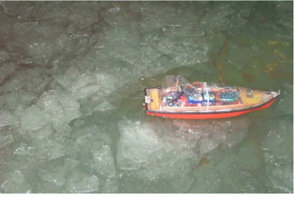
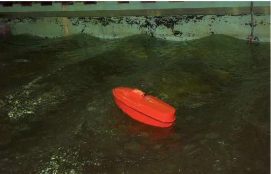
Figure 10 Mad Rock lifeboat model...12
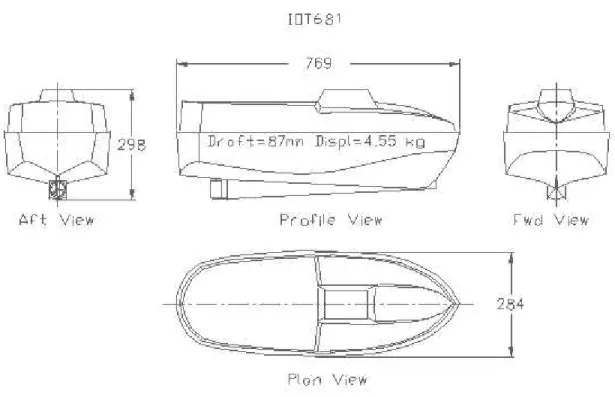
Figure 11 Scale drawings of the IOT 681 lifeboat ...13
Figure 12 Druck pressure sensor ...15
Figure 13 Motorola pressure sensor, mounted on square aluminum tubing support ...15
Figure 14 Sketch of ice tank set-up and basin co-ordinate system...17
Figure 15 Illustration of launch directions ...18
Figure 16 Example x-y output from video analysis. Note that the direction of travel is the intended direction, which not always necessarily the heading the vessel achieved...25
Figure 17 Example of wave analysis for three pressure sensors (P1, P2, and P3) used to determine wave heights for test no. 71 (CO_9_06_90_P1). ...27
Figure 18 IOT 544 test results; pass/fail criterion set at 5.0 boat-lengths ...30
Figure 19 IOT 544 test results; pass/fail criteria set at 5.0 boat-lengths and test duration of 40 seconds...30
Figure 20 IOT 609 test results; pass/fail criterion set at 5.0 boat-lengths ...31
Figure 21 IOT 609 test results; pass/fail criteria set at 5.0 boat-lengths and test duration of 40 seconds...31
Figure 22 IOT 681 test results; pass/fail criterion set at 5.0 boat-lengths ...32
Figure 23 IOT 681 test results; pass/fail criteria set at 5.0 boat-lengths and test duration of 40 seconds...32
Figure 24 IOT 681 lifeboat tests at 9/10ths ice concentration, wave frequency of 0.8 Hz, power level P1 (6 knots), and launch direction of (a) 0 degrees; (b) 90 degrees...33
Figure 25 IOT 544 lifeboat model tests at 0 minus heading, 7/10ths ice concentration, power level P1, and wave frequency of (a) 0.6 Hz; (b) 0.8 Hz; (c) 1.0 Hz. ...34
Figure 26 IOT 544 lifeboat model tests at 0 minus heading, 7/10ths ice concentration, wave frequency of 1.0 Hz, and power level of (a) P1; (b) with additional power, P2. ...36
Figure 27 IOT 609 lifeboat model tests at 90 degree heading, 9/10ths ice concentration, and wave frequency of 0.8 Hz, and power level of (a) P1; (b) with additional power, P2. ...37
Figure 28 Summary of results ...39
TESTING OF EVACUATION SYSTEM MODELS IN ICE-COVERED
WATER WITH WAVES
1. INTRODUCTION
The incorporation of escape-evacuation-rescue (EER) systems on offshore structures is an important aspect of platform design. These systems need to take into account not only a wide range of possible hazards and structure design, but also a wide range of environmental conditions. Moreover, conventional lifeboats are often the primary means of evacuation from offshore structures. While these vessels may be satisfactory in open-water conditions, the question arises as to their capabilities in ice-covered water. In these situations, the lifeboat must be able to withstand potential conditions with higher loading and limited navigability, compared to open water.
Lifeboats similar to the models tested in this study would only be used for offshore evacuation in a limited range of pack ice conditions, not in fast ice. Factors that will affect lifeboat performance in ice-covered water include the ice concentration, thickness and strength, the prevalence of land-fast or pack ice conditions, the presence of waves and the physical features of the ice. In order to evaluate the effectiveness of an evacuation system, or a part thereof, these factors must be taken into account in the design and operation of an EER system (see, for example, Poplin et al., 1998a and 1998b; Wright et al., 2003).
The presence of both ice and waves surrounding an offshore platform could occur off of the Eastern coast of Canada (the Grand Banks region), where offshore development is presently occurring. In this region, pack ice could potentially surround an offshore platform, and certainly the wave climate in this region is known to be severe. There are additional implications that make the study of lifeboat performance in ice and waves important. In the event of an emergency with toxic fumes or smoke plumes, it could become necessary for a lifeboat to travel in a specific direction, for example, upwind of the compromised structure. However, upwind is often also updrift (that is, into the waves). For these reasons, it is important to investigate the manoeuvrability of a vessel in both ice and waves, and to define the wave and ice conditions in which vessel movement is possible.
2. PROJECT OBJECTIVES AND SCOPE
The project objectives were a continuation and expansion of those of two previous test series (Simões Ré et al, 2003; Barker et al, 2004). In the first series of tests, the performance of a conventional hull design in ice was investigated, with various ice concentrations, piece sizes, ice thicknesses and with two different power capabilities. The aim was to determine performance boundaries of the lifeboat in these varying conditions. In the second test series, waves were added to some of the previous test configurations to study the effect of waves on lifeboat performance in ice. The wave period, in model scale, was either a “storm” condition of 1.0 seconds or a “swell” condition of 1.67 s.
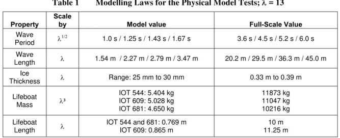
The present test series investigated three lifeboat designs: a conventional model (IOT 544), a free fall model (IOT 609), and a Mad Rock Polar Haven model (IOT 681). The models were scaled to 1:13. Table 1 shows the scaling factors for a variety of the test parameters. The characteristics that were varied in the tests were the wave period, ice concentration, launch direction, and power to the boat. The main tests were done at 7 and 9 tenths ice concentration, and the ice sheet thickness varied from 25 to 30 mm.
The wave parameters were first determined for conditions without ice. The wave height was kept constant at 0.1 m (model scale). The wave periods used, in model scale, were 1.0, 1.25, 1.43, and 1.67 seconds. These values were chosen for two reasons: (1) they are representative of moderate conditions in the Grand Banks region offshore Canada, and (2) they are at the limit of the capabilities of the wave machine in the ice tank at Canadian Hydraulics Centre.
Table 1 Modelling Laws for the Physical Model Tests; λ = 13
Property
Scale
by Model value Full-Scale Value
Wave Period λ 1/2 1.0 s / 1.25 s / 1.43 s / 1.67 s 3.6 s / 4.5 s / 5.2 s / 6.0 s Wave Length λ 1.54 m / 2.27 m / 2.79 m / 3.47 m 20.2 m / 29.5 m / 36.3 m / 45.0 m Ice Thickness λ Range: 25 mm to 30 mm 0.33 m to 0.39 m Lifeboat Mass λ³ IOT 544: 5.404 kg IOT 609: 5.028 kg IOT 681: 4.650 kg 11873 kg 11047 kg 10216 kg Lifeboat Length λ IOT 544 and 681: 0.769 m IOT 609: 0.865 m 10 m 11.25 m
The tests investigated three launch directions: the model facing into the waves (referred to as 0° Minus), away from the waves (0° Plus), or parallel to the waves (90°). For the tests in which the lifeboat was launched 90° to the direction of wave travel, the model had to turn to face into the waves and try to make headway in that direction. The launch direction was varied in order to study how well the model could make headway into the waves or how effectively it could be
The ice thicknesses investigated ranged from 25 to 30 mm in model scale. Piece size was randomly generated, in order to reflect a natural ice regime.
The effects of power to the model were also investigated in the present test program. The models were tested at power level P1 (approximately 3.1 m/s or 6 knots), and with additional power (P2). The value for power level P2 was slightly different for each lifeboat and are discussed in Section 3.4.
During several runs, the effect of using the coxswain view was investigated. In these tests, the operator attempted to drive the model using the boat view only.
Several other variables that were not intended to be investigated as part of the test program are likely to influence lifeboat performance. These variables include the ice floe size and the performance of the beaches or wave absorbers.
3. TEST SET-UP
3.1 Test Facility
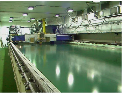
The tests were performed in the ice tank at the NRC Canadian Hydraulics Centre (CHC) in Ottawa (Pratte and Timco, 1981). Previous tests were held at the NRC Institute for Ocean Technology (IOT) (Simões Ré et al, 2003; Simões Ré et al, 2002), however the IOT ice tank is not able to accommodate a wave machine. The CHC tank, which is 21 m long by 7 m wide and 1.2 m deep, has a removable gate that facilitates access by a loader for moving the wave machines into the ice tank, and is housed in a large insulated room equipped with loading bay doors. The room can be cooled to an air temperature of -20°C. By varying the room's air temperature, ice sheets can be grown, tempered or melted. Spanning the ice tank is a carriage that can travel the length of the tank. The carriage is driven through two helical-cut rack and pinion gears, and is designed for loads up to 50 kN with a speed range from 3 to 650 mm/s. The evacuation system was mounted onto the main carriage. A small service carriage also spans the tank and this was used to mount wave gauges for sampling purposes. A photograph of the tank is shown in Figure 1.
Figure 1 Ice tank at the Canadian Hydraulics Centre.
3.2 Ice
3.2.1 Model Ice Characteristics
PG/AD model ice was used for this test series. This model ice is based on the EG/AD/S model ice developed at NRC in Ottawa (Timco 1986). PG/AD model ice represents well, on a reduced
toughness and density. The paper by Timco (1986) gives details of the mechanical properties of the model ice.
3.2.2 Ice Sheet Preparation
The thickness of the ice was adjusted by selecting an appropriate freezing time to produce the desired thickness. The strength of the ice can be adjusted by altering the time allowed for warming-up the ice. Three ice sheets were used for the test series at 5, 7 and 9 tenths concentration. Each ice sheet was used for a full day of testing. It was intended that the ice sheet be grown to 50 mm, however problems adjusting the cooling system meant that the ice sheets were grown to about 25 to 30 mm thickness.
The first ice sheet, at approximately 5/10ths concentration, was used as a test sheet but the results are analysed here. The second ice sheet was made to 7/10ths concentration. After testing the model lifeboats at this concentration, it was seen that the boats were travelling fairly easily through the ice and wave conditions. For the third day of testing, it was decided that a higher ice concentration (9/10ths) should be used in order to obtain more useful results from the experiment. In order to achieve the desired concentration of ice in the tank, large sheets of rigid insulation were laid across the tank prior to freezing. For example, at 7/10ths concentration, 30 percent of the water’s surface was covered with sheets of insulation (Figure 2).
Figure 2 Preparing an ice sheet. Rigid insulation covers the water surface in order to control the concentration of ice in the tank.
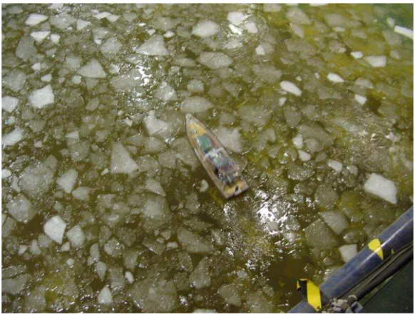
On the morning of testing the temperature in the ice tank chamber was raised to hover around 2°C. The rigid sheets of insulation were removed, and staff randomly broke the ice using rakes and hoes in order to break up the ice sheet into floes. The photo in Figure 3 is an example of a
size is approximately 0.2 m. Figure 4 shows some example floe sizes used during one test day.
The effects of ice strength were not investigated, as the focus of the testing was the manoeuvrability of the models in ice with a wave regime. Unlike previous tests that investigated the performance of the model in ice (but without waves), the ice strength was not monitored during the present test series, as there was no undisturbed ice that was suitable for performing flexural tests after the wave machines had been turned on. The ice was initially significantly stronger than a correctly-scaled ice sheet. However, in this case the higher strength implies that floe splitting would not occur if the vessel hit a floe. By the end of each test day, approximately six or seven hours after testing began, the ice was considerably weaker.
3.3 Waves
In this test series, the objective was to examine some moderate wave scenarios that may exist in the Grand Banks region offshore Canada.
3.3.1 Wave Generation
The water depth for all tests was 0.6 m. Wave generation was achieved using a computer-controlled portable wave machine. Sophisticated wave generation software permits the simulation of natural sea states as defined by parametric or measured spectra or by measured wave records.
The wave machines were operated at 0.6, 0.7, 0.8, or 1.0 Hz, corresponding to a model wave period of 1.67, 1.43, 1.25, or 1.0 seconds.
3.3.2 Wave Absorption
In order to absorb wave energy in the ice tank, Progressive Wave Absorbers were placed at the opposite end of the ice tank from the wave machines. This patented type of wave absorber was developed at the CHC in the 1980’s, and is now used in several other offshore modelling basins and towing tanks around the world. The performance of the absorber depends on its length, and on the porosities of the constituent galvanized metal sheets. In larger model basins, the absorbers’ performance is quite good, with reflection coefficients in the order of 2-6%. In the ice tank, while no measurement of the absorption of the wave energy was made, it was not anticipated that a much larger level of reflection would be observed. More details about the performance of the wave absorbers can be found in Jamieson and Mansard (1987).
In order to help prevent ice from freezing onto the wave absorbers, pieces of rigid insulation were inserted between the absorbers before the temperature of the ice tank was lowered to grow the ice sheet. Reducing the amount of ice on the absorbers ensured their good performance.
3.4 Evacuation Systems
The lifeboat models were lowered into the water using an aluminum square tubing angle with a quick release snap shackle on the model end. The intent was to look at the sail-away phase and not at the lowering and splash down. Earlier experiments used a modelled twin falls deployment system. For the present tests, the model was lowered to the water/ice surface and released from the hook. The sail-away phase was operated from the carriage above the ice tank. At the end of each test, the lifeboat was driven to the edge of the tank, where it was physically removed,
being deployed with the launching system is shown in Figure 5.
Figure 5 Lifeboat model with launching system
3.4.1 Conventional TEMPSC Design (IOT 544)
The conventional lifeboat model used in the present study was similar to that used in the previous evacuation test series at CHC (Barker et al., 2004). One main difference was the implementation of a new drive system, explained further in Section 4.3. A summary of the model’s main features is presented here. The model had a scale of 1:13 and was representative of a 10 m long 80-person totally enclosed motor propelled survival craft (TEMPSC). In model scale the vessel was 0.769 m long with a mass of 5.4 kg, representing a full complement of evacuees. A photograph of the model is shown in Figure 6, with scale drawings in Figure 7.
The model was tested at two different levels of power. Power level P1, at 2600 rpm, corresponded to 1.2 Newton bollard pull and a model speed of 0.86 m/s or 1.7 knots. The vessel was also tested with additional power P2 at 3700 rpm, corresponding to 2.7 Newton bollard pull and a speed of 1.1 m/s (2.1 knots).
Figure 7 Scale drawings of the IOT 544 lifeboat model
3.4.2 Free fall TEMPSC design (IOT 609)
The IOT 609 model had a scale of 1:13 and was representative of a 11.25 m long lifeboat with an 80-person capacity. The model vessel was 0.865 m long, and was tested for a full complement of evacuees (model mass of 5.03 kg). A photograph of the IOT 609 model is shown in Figure 8. Scale drawings of the model are shown in Figure 9. The model had a four-bladed propeller with 70 mm diameter, an active rudder, an electric motor and shaft, rechargeable batteries, a wireless video camera and a radio transmitter.
The IOT 609 model was tested with two different levels of power. Power level P1 was at 2500 rpm, corresponding with 1.0 Newton bollard pull and a speed of 0.86 m/s (1.7 knots). The vessel was also tested with additional power (P2) at 3700 rpm, corresponding to 2.4 Newton bollard pull and a speed of 1.1 m/s (2.2 knots).
Figure 8 IOT 609 lifeboat model
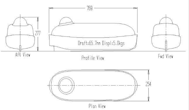
The Polar Haven line of TEMPSCs from Mad Rock Marine Solutions are designed to have a higher performance in ice covered waters and severe environmental conditions. A higher power engine coupled with a high torque propeller were used to provide better manoeuvring characteristics in the above mentioned water conditions. A forward placed coxswain station allows the pilot better visibility of ice and debris. The model is designed for roll reduction and ice protection for the propeller, and a forward placed ice knife helps to prevent the hull from beaching upon ice during transport through ice floes. A photograph of the IOT 681 lifeboat model tested during this study is shown Figure 10, with scale drawings shown in Figure 11.
The IOT 681 model had a scale of 1:13, representing a 10m long lifeboat with a capacity of 64 people. In model scale, the vessel was 0.769 m long and ballasted to a mass of 4.65 kg, representing a full complement of evacuees. The propeller for the model lifeboat was 70 mm in diameter with 3 blades. Like the other designs, the IOT 681 model had a steerable nozzle, an electric motor and shaft, rechargeable batteries, a wireless video camera and a radio transmitter. The IOT 681 TEMPSC model was tested with two different levels of power. Power level P1, at 2300 rpm, corresponded to 1.19 Newton bollard pull and a speed of 0.86 m/s (1.7 knots). The vessel was also tested with additional power P2 at 3700 rpm, corresponding to 3.45 Newton bollard pull and a speed of 1.1 m/s (2.2 knots).
4. INSTRUMENTATION
The instrumentation used to collect data during the test series was as follows: For the lifeboats:
• Three accelerometers recording longitudinal, lateral and vertical accelerations • Three rate gyros monitoring roll, pitch and yaw
• Motor controller
• Boat-mounted video camera • Radio transmitter
For the ice tank:
• Three pressure sensors
• Two overhead video cameras to track X-Y position of model
Note that only the pressure sensor and overhead video data were analysed for this study. All analog sensors were calibrated before the start of the experiments. Some of these systems are described in further detail below.
4.1 Wave Data Acquisition
The intent for this series was not to continually monitor the wave conditions, but rather to attempt to reproduce realistic wave climates. The wave height and periods used in this test series were based on un-damped values, that is, with no ice. Because of the dampening effect of pack ice on waves, an attempt was made to measure the wave heights that occurred during testing.
For the last series of tests at the CHC, two capacitance-type wave probes were used to measure wave heights. Protective coverings made of wire mesh were constructed in order to prevent ice from directly interacting with the probes. It was not always possible to prevent this occurrence however, and by the end of the test program, ice was routinely becoming stuck in the protective cages (Barker et al., 2004).
For the present test series, three pressure sensors (P1, P2, and P3) were used to measure wave heights. Since the sensors are submersible, ice impacts are not an issue. The sensors were located along the centreline of the tank, with sensors P1 and P3 located 4.5 m from the wave generator, and sensor P2 located 5.16 m from the wave generator.
Two different types of pressure sensors were used for measuring wave height in the experiments. Sensors P1 and P2 were Motorola MPX2050 Series devices. The accuracy over the calibration range for wave elevations of 0 m to 0.4 m was approximately ± 0.084% for P1 and ± 0.79% for P2. Sensor P3 was a Druck PDCR1830 Series depth-sensing transducer with ± 0.1% accuracy. Photographs of the two types of pressure sensors are shown in Figure 12 and Figure 13. The sensors were mounted on supports to keep them approximately 10 cm above the floor of the test basin.
Figure 12 Druck pressure sensor
Figure 13 Motorola pressure sensor, mounted on square aluminum tubing support
4.2 TEMPSC Data Acquisition
A newly developed 16-channel 16-bit resolution data acquisition system was implemented for this round of testing at CHC. It was set up to sample 12 channels at a rate of 320 Hz. See Table 2 for channel list and range.
Channel Device Range
1 Surge Acceleration 10 g
2 Sway Acceleration 10 g
3 Heave Acceleration 8 g
4 Roll Rate 300 deg/sec
5 Pitch Rate 300 deg/sec
6 Yaw Rate 300 deg/sec
7 RPM 0 - 4000
8 Not used N/A
9 Battery voltage 0 - 25 Volts
10 Battery current 0 - 3 Amps
11 Rudder angle +/- 30 Deg
12 Not used N/A
The data was digitized on board the model and transmitted via a 433Mhz radio link to the data logging software on a computer outside the ice tank. The transmit protocol, with its error checking and an advanced receiver design, had an average data capture rate with over 99% effectiveness. This radio system has proven to be reliable in cold and wet environments as well as in areas with multiple metal structures.
The sensors used to acquire acceleration and rates were small capacitive micro-machined units featuring low power consumption. The RPM sensor was a non-contact magnetic-type unit that also outputs direction. The motor voltage supply level came from a resistor network and the drive motor current was derived from a sensor that used a high-side current-sense amplifier across an internal resistor. The rudder angle was derived from a mechanically coupled potentiometer that is powered by a precision voltage reference.
4.3 TEMPSC Remote Control and Drive Systems
The control system was newly developed for this series of tests, replacing the hand held “hobby unit” that was used in the previous evacuation model tests at CHC.
The new design allowed for interfacing with the PC-based controller software. This software enabled each model to be operated with its unique set of calibrated command inputs, and the data file saved for future testing. Another benefit was the quick change over from one model to the next, each sharing the common control system hardware. The software also provided a more realistic and advanced form of human interface that includes a joystick and steering wheel. The control link was achieved through a wireless radio transmitter at 2.4 GHz using “Blue tooth” encoding.
The drive systems on all three models were also updated to include a 44-watt motor with a programmable integrated controller. This gave the models reverse capability and excellent RPM control, both of which were lacking in the previous version. The implementation of this new drive
programmable digital servo, allowing the operator to program the maximum slew rate, range of travel and centre position of the rudder.
4.4 Co-ordinate Systems
4.4.1 Basin Co-ordinates
For the test basin, the co-ordinate system was right-handed. The positive X-axis is defined as up the tank towards the wave absorbers, the Y-axis is defined as the direction perpendicular to the carriage, and the Z-axis is upwards. This is illustrated in Figure 14. Figure 15 is an illustration of the launch directions.
Figure 14 Sketch of ice tank set-up and basin co-ordinate system
4.4.2 TEMPSC Co-ordinates
Each TEMPSC model had a fixed system, with the origin at the aft of the keel along the centre line. This right-handed coordinate system is fixed to the TEMPSC and moves with it. It defines the location of equipment in the TEMPSC, the location of the release mechanisms, the wireless camera position and the accelerometers. Further details about this system were provided in a previous study (Simões Ré et al, 2003). The motion pack was located close to the centre of gravity within the TEMPSC models.
0° Minus Launch
(into waves, travel towards wave machines)
90° Launch
0° Plus Launch
(with waves, travel towards wave absorbers)
Figure 15 Illustration of launch directions
4.5 Video
Two video cameras were mounted over the test area of the ice tank. The purpose of mounting the cameras in this manner was to use the resulting videos to track the x-y movement of the lifeboat. The cameras were spaced such that a total travel distance of approximately 5.5 m was covered by the two cameras combined. The field of view of the cameras was such that the entire width of the ice tank could not be covered. If the lifeboat drifted or was propelled a wide distance off the centerline of the tank, the lifeboat could no longer be observed by the cameras and this portion of the vessel track would be lost. Also, if the lifeboat was pushed under the service carriage by the waves it was no longer visible to the cameras. Some video data was also collected from a tripod-mounted camera at one end of the ice tank. However, this data is suitable for qualitative analysis only (whether the model met the pass/fail criteria), not x-y positioning.
The video camera located onboard the TEMPSC had, in previous tests, been used by the lifeboat operator to provide the same view as the TEMPSC coxswain. For the present test series, as in the 2003 test series at CHC, the operator chose to operate the TEMPSC lifeboat from atop the main carriage in the ice tank. The lifeboat was navigated by looking down on it, rather than using the view from the on-board camera. The on-board camera view was insufficient for navigating in waves and ice. This decision is discussed further in Section 7.
5. TEST PROGRAM
5.1 Test Methodology
The test methodology was similar to the previous test series, and proceeded as follows: • The test configuration was set according to the matrix.
• The lifeboat was lowered to water level
• The lifeboat data acquisition was started, followed by the lifeboat video. • The overhead video recording was started.
• The pressure sensor data acquisition was started.
• The wave machines were initiated with the appropriate drive signal.
• After a manual signal was received, the deployment started. Half way between the lifeboat launching rest position and the water surface, the lifeboat propulsion system was started remotely. The deployment start coincided with the start of the wave machines as much as possible.
• The launching mechanism released the lifeboat into the water. The vessel operator exercised the rudder control remotely during the lifeboat sail away to the safe zone. • After the TEMPSC either reached the safe zone or it could not travel any further, the
wave machines and other data acquisition systems were stopped.
• After completion of the test, the members of the project team started preparation for the next run. The lifeboat was manoeuvred to the edge of the tank, where it was lifted out and reconnected to the launch system.
• The ice in the tank was raked back across the tank to re-cover the water surface.
• The time between test runs was approximately 10 minutes when all events ran smoothly.
5.2 Test Matrix
The complete test matrix consisted of testing three ice sheets. A total of 126 tests were performed. Table 3 shows the 106 tests that were the primary focus of the laboratory program. Tests not included in Table 3 are those that were performed with no power or in still water. Details of all of the tests for the conventional (IOT 544), free fall (IOT 609), and Mad Rock (IOT 681) lifeboat models are shown in Table 4, Table 5, and Table 6 respectively. Tests were named as in the example below. A full explanation of the test names may be found in Appendix B. CO_5_06_0MINUS_P1
CO conventional lifeboat model (IOT 544) 5 ice concentration in tenths [5/10ths]
06 wave frequency in Hz [0.6 Hz]
0MINUS launch direction [0 minus, or into waves]
ice was mainly used for preliminary testing purposes but several tests at the 0-minus heading (launching into the waves) were carried out. Results from these tests are included here. Since there were several variables to be tested, there was not enough time to perform all tests more than once.
Table 3 Main test matrix
Number of tests performed for each lifeboat Launch direction
(degrees)
Nominal ice concentration
(tenths) IOT 544 IOT 609 IOT 681
0- 5 8 6 6 7 5 5 6 9 9 9 9 0+ 5 - - - 7 - - - 9 2 2 3 90 5 - - - 7 7 6 7 9 4 5 7
Table 4 Expanded details for the complete test matrix for the IOT 544 lifeboat model
Test # Test Name Date
Nominal Ice Concentration (tenths) Launch Direction (degrees) Power (P1/P2) Nominal Wave Height (m) Nominal Wave Frequency (Hz)
CO_0 CO_test1 18-May-05 5 0- P1 then P2 - -
1 CO_5_06_0MINUS_P1 18-May-05 5 0- P1 0.1 0.6 2 CO_5_06_0MINUS_P2 18-May-05 5 0- P2 0.1 0.6 3 CO_5_07_0MINUS_P1 18-May-05 5 0- P1 0.1 0.7 4 CO_5_07_0MINUS_P2 18-May-05 5 0- P2 0.1 0.7 5 CO_5_08_0MINUS_P1 18-May-05 5 0- P1 0.1 0.8 6 CO_5_08_0MINUS_P2 18-May-05 5 0- P2 0.1 0.8
CO_A CO_TESTA 18-May-05 5 0- P1 - -
CO_B CO_TESTB 18-May-05 5 0- P2 - -
7 CO_5_10_0MINUS_P1 18-May-05 5 0- P1 0.1 1.0 8 CO_5_10_0MINUS_P2 18-May-05 5 0- P2 0.1 1.0 21 CO_7_06_0MINUS_P1 20-May-05 7 0- P1 0.1 0.6 22 CO_7_08_0MINUS_P1 20-May-05 7 0- P1 0.1 0.8 23 CO_7_08_0MINUS_P2 20-May-05 7 0- P2 0.1 0.8 24 CO_7_10_0MINUS_P1 20-May-05 7 0- P1 0.1 1.0 25 CO_7_10_0MINUS_P2 20-May-05 7 0- P2 0.1 1.0 26 CO_7_06_90_P1 20-May-05 7 90 P1 0.1 0.6 27 CO_7_06_90_P2 20-May-05 7 90 P2 0.1 0.6 28 CO_7_08_90_P1 20-May-05 7 90 P1 0.1 0.8 29 CO_7_08_90_P2 20-May-05 7 90 P2 0.1 0.8 30 CO_7_08_90_P2A 20-May-05 7 90 P2 0.1 0.8 31 CO_7_10_90_P2 20-May-05 7 90 P2 0.1 1.0 32 CO_7_10_90_P1 20-May-05 7 90 P1 0.1 1.0 57 CO_9_06_0MINUS_P1 25-May-05 9 0- P1 0.1 0.6 58 CO_9_06_0MINUS_P2 25-May-05 9 0- P2 0.1 0.6 59 CO_9_08_0MINUS_P1 25-May-05 9 0- P1 0.1 0.8 60 CO_9_08_0MINUS_P2 25-May-05 9 0- P2 0.1 0.8 61 CO_9_07_0MINUS_P1 25-May-05 9 0- P1 0.1 0.7 62 CO_9_07_0MINUS_P2 25-May-05 9 0- P2 0.1 0.7 63 CO_9_10_0MINUS_P1 25-May-05 9 0- P1 0.1 1.0 64 CO_9_10_0MINUS_P2 25-May-05 9 0- P2 0.1 1.0 65 CO_9_06_0PLUS_P1 25-May-05 9 0+ P1 0.1 0.6 66 CO_9_08_0PLUS_P1 25-May-05 9 0+ P1 0.1 0.8
CO_C CO_9_CALM_P1 25-May-05 9 0- P1 - -
CO_D CO_9_CALM_P2 25-May-05 9 0- P2 - -
67 CO_9_08_90_P1 25-May-05 9 90 P1 0.1 0.8 68 CO_9_10_90_P2 25-May-05 9 90 P2 0.1 1.0 69 CO_9_08_90_P1A 25-May-05 9 90 P1 0.1 0.8 70 CO_9_08_0MINUS_P1A 25-May-05 9 0- P1 0.1 0.8 71 CO_9_06_90_P1 25-May-05 9 90 P1 0.1 0.6 72 CO_9_10_0PLUS_NP 25-May-05 9 0+ - 0.1 1.0
Test # Test Name Date Nominal Ice Concentration (tenths) Launch Direction (degrees) Power (P1/P2) Nominal Wave Height (m) Nominal Wave Frequency (Hz) 9 FF_5_06_0MINUS_P1 18-May-05 5 0- P1 0.1 0.6 10 FF_5_06_0MINUS_P2 18-May-05 5 0- P2 0.1 0.6 11 FF_5_08_0MINUS_P1 18-May-05 5 0- P1 0.1 0.8 12 FF_5_08_0MINUS_P2 18-May-05 5 0- P2 0.1 0.8 13 FF_5_10_0MINUS_P1 18-May-05 5 0- P1 0.1 1.0 14 FF_5_10_0MINUS_P2 18-May-05 5 0- P2 0.1 1.0
FF_A FF_TESTA 18-May-05 5 0- P1 - -
FF_B FF_TESTB 18-May-05 5 0- P2 - - 33 FF_7_06_0MINUS_P1 20-May-05 7 0- P1 0.1 0.6 34 FF_7_08_0MINUS_P1 20-May-05 7 0- P1 0.1 0.8 35 FF_7_08_0MINUS_P2 20-May-05 7 0- P2 0.1 0.8 36 FF_7_10_0MINUS_P1 20-May-05 7 0- P1 0.1 1.0 37 FF_7_10_0MINUS_P2 20-May-05 7 0- P2 0.1 1.0 38 FF_7_06_90_P1 20-May-05 7 90 P1 0.1 0.6 39 FF_7_06_90_P2 20-May-05 7 90 P2 0.1 0.6 40 FF_7_08_90_P1 20-May-05 7 90 P1 0.1 0.8 41 FF_7_08_90_P2 20-May-05 7 90 P2 0.1 0.8 42 FF_7_10_90_P1 20-May-05 7 90 P1 0.1 1.0 43 FF_7_10_90_P2 20-May-05 7 90 P2 0.1 1.0 FF_C FF_7_CALM_0MINUS_P1 20-May-05 7 0- P1 - - FF_D FF_7_CALM_0MINUS_P2 20-May-05 7 0- P2 - - 73 FF_9_06_0MINUS_P1 25-May-05 9 0- P1 0.1 0.6 74 FF_9_06_0MINUS_P2 25-May-05 9 0- P2 0.1 0.6 75 FF_9_08_0MINUS_P1 25-May-05 9 0- P1 0.1 0.8 76 FF_9_08_0MINUS_P2 25-May-05 9 0- P2 0.1 0.8 77 FF_9_07_0MINUS_P1 25-May-05 9 0- P1 0.1 0.7 78 FF_9_07_0MINUS_P2 25-May-05 9 0- P2 0.1 0.7 79 FF_9_10_0MINUS_P1 25-May-05 9 0- P1 0.1 1.0 80 FF_9_10_0MINUS_P2 25-May-05 9 0- P2 0.1 1.0 81 FF_9_06_90_P1 25-May-05 9 90 P1 0.1 0.6 82 FF_9_08_90_P1 25-May-05 9 90 P1 0.1 0.8 83 FF_9_08_90_P2 25-May-05 9 90 P2 0.1 0.8 84 FF_9_10_90_P2 25-May-05 9 90 P2 0.1 1.0
FF_E FF_9_CALM_P2 25-May-05 9 0- P2 - -
FF_F FF_9_CALM_P1 25-May-05 9 0- P1 - - 85 FF_9_08_90_P1 25-May-05 9 90 P1 0.1 0.8 86 FF_9_10_0MINUS_P1A 25-May-05 9 0- P1 0.1 1.0 87 FF_9_06_0PLUS_P1 25-May-05 9 0+ P1 0.1 0.6 88 FF_9_08_0PLUS_P1 25-May-05 9 0+ P1 0.1 0.8 89 FF_9_10_0PLUS_NP 25-May-05 9 0+ - 0.1 1.0
Table 6 Expanded details for the complete test matrix for the IOT 681 lifeboat model
Test # Test Name Date
Nominal Ice Concentration (tenths) Launch Direction (degrees) Power (P1/P2) Nominal Wave Height (m) Nominal Wave Frequency (Hz) 15 MR_5_06_0MINUS_P1 18-May-05 5 0- P1 0.1 0.6 16 MR_5_06_0MINUS_P2 18-May-05 5 0- P2 0.1 0.6 17 MR_5_08_0MINUS_P1 18-May-05 5 0- P1 0.1 0.8 18 MR_5_08_0MINUS_P2 18-May-05 5 0- P2 0.1 0.8 19 MR_5_10_0MINUS_P1 18-May-05 5 0- P1 0.1 1.0 20 MR_5_10_0MINUS_P2 18-May-05 5 0- P2 0.1 1.0
MR_A MR_TESTA** 18-May-05 5 0- P1 - -
MR_B MR_TESTB** 18-May-05 5 0- P2 - - 44 MR_7_06_0MINUS_P1 20-May-05 7 0- P1 0.1 0.6 45 MR_7_08_0MINUS_P1 20-May-05 7 0- P1 0.1 0.8 46 MR_7_08_0MINUS_P2 20-May-05 7 0- P2 0.1 0.8 47 MR_7_10_0MINUS_P1 20-May-05 7 0- P1 0.1 1.0 48 MR_7_10_0MINUS_P1A 20-May-05 7 0- P1 0.1 1.0 49 MR_7_10_0MINUS_P2 20-May-05 7 0- P2 0.1 1.0 50 MR_7_06_90_P1 20-May-05 7 90 P1 0.1 0.6 51 MR_7_06_90_P2 20-May-05 7 90 P2 0.1 0.6 52 MR_7_08_90_P1 20-May-05 7 90 P1 0.1 0.8 53 MR_7_08_90_P2 20-May-05 7 90 P2 0.1 0.8 54 MR_7_10_90_P1 20-May-05 7 90 P1 0.1 1.0 55 MR_7_10_90_P1A 20-May-05 7 90 P1 0.1 1.0 56 MR_7_10_90_P2 20-May-05 7 90 P2 0.1 1.0 MR_C MR_7_CALM_0MINUS_P1 20-May-05 7 0- P1 - - MR_D MR_7_CALM_0MINUS_P2 20-May-05 7 0- P2 - - 90 MR_9_06_0PLUS_P1 25-May-05 9 0+ P1 0.1 0.6 91 MR_9_08_0PLUS_P1 25-May-05 9 0+ P1 0.1 0.8 92 MR_9_10_0PLUS_NP 25-May-05 9 0+ - 0.1 1.0 93 MR_9_06_0MINUS_P1 25-May-05 9 0- P1 0.1 0.6 94 MR_9_06_0MINUS_P2 25-May-05 9 0- P2 0.1 0.6 95 MR_9_08_0MINUS_P1 25-May-05 9 0- P1 0.1 0.8 96 MR_9_08_0MINUS_P2 25-May-05 9 0- P2 0.1 0.8 97 MR_9_07_0MINUS_P1 25-May-05 9 0- P1 0.1 0.7 98 MR_9_07_0MINUS_P2 25-May-05 9 0- P2 0.1 0.7 99 MR_9_10_0MINUS_P1 25-May-05 9 0- P1 0.1 1.0 100 MR_9_10_0MINUS_P2 25-May-05 9 0- P2 0.1 1.0 101 MR_9_06_90_P1 25-May-05 9 90 P1 0.1 0.6 102 MR_9_08_90_P1 25-May-05 9 90 P1 0.1 0.8 103 MR_9_10_90_P2 25-May-05 9 90 P2 0.1 1.0
MR_E MR_9_CALM_P2 25-May-05 9 0- P2 - -
MR_F MR_9_CALM_P1 25-May-05 9 0- P1 - - 104 MR_9_10_0MINUS_P2A 26-May-05 9 0- P2 0.1 1.0 105 MR_9_06_90_P1A 26-May-05 9 90 P1 0.1 0.6 106 MR_9_08_90_P1A 26-May-05 9 90 P1 0.1 0.8 107 MR_9_10_90_P2 26-May-05 9 90 P2 0.1 1.0 108 MR_9_10_90_P2A 26-May-05 9 90 P2 0.1 1.0 109 MR_9_06_0PLUS_P1A 26-May-05 9 0+ P1 0.1 0.6
6. RESULTS
A complete summary of the results of the test program for the three lifeboat designs (conventional, free fall and Mad Rock) may be found in Appendices C, D and E, respectively. These appendices contain tables of data that summarize the pass/fail results for each test as well as the x-y plots of the vessel’s travel path. Appendix H shows some general photographs from the tests.
As with the previous tests in ice, successful runs were defined as those for which the TEMPSC was able to launch and then sail away a set distance through the broken ice. Each test in this series was given a pass or fail grade based on whether the boat made it to a distance of 5.0 boat lengths from its launch point target. This corresponds to a full-scale distance of 50 m for the conventional (IOT 544) and Mad Rock (IOT 681) models, and 56 m for the free fall (IOT 609) model.
6.1 Video Analysis
The overhead video was recorded on VHS tapes for the first day of testing, and on DVD for the remaining test days. The VHS videos were converted from analog to digital video. The video logs for all tests are found in Appendix F.
Once the videos had been screened, the video segment for each test was recorded in digital format and exported as an .avi file. The video was not slowed down to convert it to full-scale time. These .avi files were then used in a program called VideoPoint Capture, allowing a specific number of frames to be selected for analysis. Typically 5 to 10 frames were determined to be sufficient for x-y plotting purposes. The digital video files were then compressed and saved. Finally, the compressed files were opened in VideoPoint 2.5. The x-y axes were rotated for each file, since the cameras were not perfectly aligned with the tank. The path of the vessel was then traced using the digital tracking capabilities of this program. For each frame, a point on the vessel had to be highlighted. Each point was represented by a set of x-y coordinates and the corresponding time. This data was exported to Excel and plotted as a representation of the path of the motion of the model.
The data manipulation in Excel was fairly straightforward. A correction was made to the data for each test before plotting. The two overhead cameras were positioned such that the vessel traveled from one camera’s field of view into the other. The fields of view of the two cameras overlapped, so the two sets of data had to be superimposed and then made into one continuous data set. Also, the plotting order of the points from camera A and camera B depended on the direction of travel of the vessel. For motion in the positive direction (i.e. with the waves) data from camera B had to be listed before camera A and for a negative vessel direction (into the waves) data points for camera A were plotted before camera B. An example of a typical output plot is shown in Figure 16. The coloured, dotted lines indicate the location of 2.5, 5.0 and 7.5 boat lengths of travel distance. The red diamond indicates the launch location. Note that the direction of travel indicates the intended direction for the lifeboat, either into or with the waves, not the direction that the lifeboat may have ended up traveling.
was often blocked by the main service carriage from which the vessel was launched. Thus, for some tests the boat did not appear to quite meet the 5.0 boat length distance required for a ‘pass’. Most of these tests were obviously actually ‘passes’. If a test was questionable, the video taken from the end of the tank could be examined.
Figure 16 Example x-y output from video analysis. Note that the direction of travel is the intended direction, which not always necessarily the heading the vessel achieved.
CO_5_06_0MINUS_P2 -2 -1.5 -1 -0.5 0 0.5 1 1.5 2 0 1 2 3 4 5 X [m] Y [ m ] 6 Wave direction Direction of travel Launch point
2.5 boat lengths 5.0 boat lengths 7.5 boat lengths
6.2 Pressure Sensor Data Analysis
An example of wave analysis for one test is shown in Figure 17. Plots of the analysed pressure sensor data can be found in Appendix E.
In the 2003 evacuation test series, the wave probe readings were unreliable because the ice routinely jammed the protective cages surrounding the wave probes. Where good readings were obtained, the storm wave heights were generally much lower than the 0.1 m nominal height, with values ranging from 0.01 m to 0.04 m. The swell readings, by contrast, were much higher than the nominal wave height, often almost three times as large. This could be due to the generation of standing waves in the ice tank under swell conditions (Barker et al., 2004).
In the present test series, most values for maximum wave height were closer to the 0.1m nominal wave height, although on average all were higher than the nominal height. The average maximum wave heights were quite high for the 1-second period swell waves (1.0 Hz) at 5/10ths
wave heights for various ice conditions.
Table 7 Average maximum wave heights (m) for various conditions in the ice tank Ice concentration Wave frequency 5/10ths 7/10ths 9/10ths 0.6 Hz 0.148 0.116 0.120 0.7 Hz 0.154 - 0.121 0.8 Hz 0.179 0.165 0.157 1.0 Hz 0.232 0.243 0.167
0 20 40 60 80 100 120 -0.06 -0.04 -0.02 0 0.02 0.04 0.06 0.08 Time (s) W a v e he ight (m ) P3 0 20 40 60 80 100 120 -0.06 -0.04 -0.02 0 0.02 0.04 0.06 Time (s) W av e he ig ht ( m ) P1 0 20 40 60 80 100 120 -0.06 -0.04 -0.02 0 0.02 0.04 0.06 0.08 Time (s) W a v e he ight (m ) P2
Figure 17 Example of wave analysis for three pressure sensors (P1, P2, and P3) used to determine wave heights for test no. 71 (CO_9_06_90_P1).
7. DISCUSSION
7.1 Effect of Waves and Ice Combined
Table 8 shows the results for tests in the main test matrix (those indicated in Table 4, 5 and 6). In the table, an “F” indicates a fail while a “P” indicates a pass. These grades are preceded by the number of tests in that configuration that received that grade. The pass criterion was that the vessel reaches a distance of 5.0 boat lengths in the intended direction of travel. Results with an asterisk (*) indicate that overhead video data was missing for one or more tests. Where available, video taken from the end of the tank was used to assess whether the vessel had a probable pass or fail.
Table 8 Results for the main test matrix; pass/fail criterion set at 5.0 boat-lengths Grade for each lifeboat [Pass or Fail] Launch
direction (degrees)
Nominal ice concentration
(tenths) IOT 544 IOT 609 IOT 681
0- 5 7P 1F* 6P 6P 7 4P 1F 5P 6P 9 8P 1F 9P 8P 1F** 0+ 5 - - - 7 - - - 9 2P 2P 2P* 90 5 - - - 7 7P 6P 6P* 9 3P 1F 4P 1F 4P 3F**
* missing overhead video analysis for one or more tests ** failure may be due to rudder problems in at least one test
The lifeboat models each had difficulty getting through the waves and ice for some tests. The average test duration for a ‘pass’ using the 5 boat length criteria is approximately 30 seconds. Therefore a duration of 40 seconds was chosen (somewhat arbitrarily) as a cut-off value for pass/fail in Table 9. In model scale, this corresponds to an average speed of approximately 0.13 m/s. The full-scale lifeboat speed would be approximately 0.36 m/s, which is quite slow. For open water transit in calm conditions, the model vessels should travel at about 0.86 m/s (3.1 m/s in full-scale).
A test was considered a ‘fail’ if the boat took more than 40 seconds to reach 5 boat lengths. This method of analysis gives some indication of which factors may cause navigational problems for the vessels.
Table 9 Results for the main test matrix; pass/fail criteria set at 5.0 boat-lengths and test duration of 40 seconds
Grade for each lifeboat [Pass or Fail] Launch
direction (degrees)
Nominal ice concentration
(tenths) IOT 544 IOT 609 IOT 681
0- 5 6P 2F* 5P 1F 5P 1F 7 4P 1F 5P 5P 1F 9 5P 4F 7P 2F 7P 2F** 0+ 5 - - - 7 - - - 9 2P 2P 2P* 90 5 - - - 7 4P 3F 4P 2F 5P 1F* 9 1P 3F 2P 3F 4P 3F**
* missing overhead video analysis for one or more tests ** failure may be due to rudder problems in at least one test
7.2 Navigation of Lifeboat Models
The test results for the lifeboats were determined using pass/fail criteria of (a) reaching a distance of 5.0 boat lengths; and (b) reaching this distance within 40 seconds. Results are plotted for each model – IOT 544 (Figure 18 and Figure 19), IOT 609 (Figure 20 and Figure 21), and IOT 681 (Figure 22 and Figure 23). The tests included in the plots are those in which the vessel attempted into travel into the wave direction (from a launch heading of either 0 degrees or 90 degrees to the wave direction). Tests in which the vessel was traveling with the waves (0 plus) were excluded. There were not any major differences in the navigational capabilities of the three boats. The conventional lifeboat had more difficulty meeting the pass criteria than the IOT 609 and IOT 681 vessels. The IOT 681 model had some mechanical problems during two tests, which may have prevented the model from being able to achieve a ‘pass’. In tests 103 and 108, the IOT 681 model rudder was not operating properly. These tests were both at 9/10ths ice concentration with 1.0 Hz wave frequency.
0.4 0.5 0.6 0.7 0.8 0.9 1 1.1 4 5 6 7 8 9 10
Ice concentration (tenths)
W ave f req u en cy (H z )
Pass (reached 5 boat lengths) Fail
Figure 18 IOT 544 test results; pass/fail criterion set at 5.0 boat-lengths
0.4 0.5 0.6 0.7 0.8 0.9 1 1.1 1.2 4 5 6 7 8 9 10
Ice concentration (tenths)
W a ve f req u e n cy ( H z)
Pass (reached 5 boat lengths in <= 40 seconds)
Fail
Figure 19 IOT 544 test results; pass/fail criteria set at 5.0 boat-lengths and test duration of 40 seconds
0.4 0.5 0.6 0.7 0.8 0.9 1 1.1 1.2 4 5 6 7 8 9 10
Ice concentration (tenths)
W ave f req u en cy (H z )
Pass (reached 5 boat lengths) Fail
Figure 20 IOT 609 test results; pass/fail criterion set at 5.0 boat-lengths
0.4 0.5 0.6 0.7 0.8 0.9 1 1.1 1.2 4 5 6 7 8 9 10
Ice concentration (tenths)
W ave f req u e n cy ( H z )
Pass (reached 5 boat lengths in <= 40 seconds)
Fail
Figure 21 IOT 609 test results; pass/fail criteria set at 5.0 boat-lengths and test duration of 40 seconds
0.4 0.5 0.6 0.7 0.8 0.9 1 1.1 4 5 6 7 8 9 10
Ice concentration (tenths)
W a ve f re q u e nc y ( H z )
Pass (reached 5 boat lengths) Fail
Figure 22 IOT 681 test results; pass/fail criterion set at 5.0 boat-lengths
0.4 0.5 0.6 0.7 0.8 0.9 1 1.1 1.2 4 5 6 7 8 9 10
Ice concentration (tenths)
Wa v e f re que nc y (H z )
Pass (reached 5 boat lengths in <= 40 seconds)
Fail
Figure 23 IOT 681 test results; pass/fail criteria set at 5.0 boat-lengths and test duration of 40 seconds
7.3 Effect of Launch Direction
When travelling with the waves (0 plus heading), the model always achieved the safe distance from the start point, and was helped along by the waves. In attempting to travel into the waves (0 minus), the equivalent safe distance in the other direction was usually achieved. For the 90° launch tests, all vessels had some difficulty meeting the pass criteria at 9/10ths ice concentration and high frequency waves. Figure 24 shows the IOT 681 model’s path for two tests with the same conditions but with different launch headings. Launching the vessel at 90 degrees generally increased the length of time necessary for the lifeboat to reach a set distance, since the lifeboat had to turn to face into the wave direction without being pushed back by the waves and ice.
MR_9_08_0MINUS_P1 -2 -1.5 -1 -0.5 0 0.5 1 1.5 2 0 1 2 3 4 5 6 X [m] Y [ m ] Wave direction Direction of travel MR_9_08_90_P1 -2 -1.5 -1 -0.5 0 0.5 1 1.5 2 -1 0 1 2 3 4 5 X [m] Y [ m ] Wave direction Direction of travel (b) Time = 34 seconds (a) Time = 24 seconds
Figure 24 IOT 681 lifeboat tests at 9/10ths ice concentration, wave frequency of 0.8 Hz, power level P1 (6 knots), and launch direction of (a) 0 degrees; (b) 90 degrees
7.4 Effect of Wave Frequency on Lifeboat Performance
A higher wave frequency (i.e. shorter wave period) generally caused an increase in the time necessary for the lifeboat to travel the specified distance. The IOT 544 lifeboat model was able to pass 5.0 boat lengths in all but four tests – these four ‘fails’ were all tests at the highest wave frequency. An example of three tests with the IOT 544 model in which the wave frequency was varied is shown in Figure 25.
CO_7_08_0MINUS_P1 -2 -1.5 -1 -0.5 0 0.5 1 1.5 2 -1 0 1 2 3 4 5 X [m] Y [ m ] Wave direction Direction of travel CO_7_06_0MINUS_P1 -2 -1.5 -1 -0.5 0 0.5 1 1.5 2 0 1 2 3 4 5 6 X [m] Y [ m ] Wave direction Direction of travel (Frequency = 0.8 Hz) (Frequency = 0.6 Hz)
(a) Time = 19 seconds (b) Time = 28 seconds
(c) Time = 28 seconds CO_7_10_0MINUS_P1 -2 -1.5 -1 -0.5 0 0.5 1 1.5 2 -1 0 1 2 3 4 5 X [m] Y [ m ] Wave direction Direction of travel (Frequency = 1.0 Hz)
Figure 25 IOT 544 lifeboat model tests at 0 minus heading, 7/10ths ice concentration, power level P1, and wave frequency of (a) 0.6 Hz; (b) 0.8 Hz; (c) 1.0 Hz.
For the IOT 609 lifeboat, the model failed to reach the 5.0 boat length criterion for only one test. This test was performed at the highest wave frequency, 1.0 Hz. For all other tests, when other variables were held constant, the time taken to reach 5.0 boat lengths increased when wave frequency was increased.
For the IOT 681 model, three of the four tests in which the lifeboat failed to reach 5.0 boat lengths were tests carried out at the highest wave frequency. It is noted that this model experienced some mechanical difficulties, which may have prevented the lifeboat from performing properly in two of the tests that appeared to be ‘fails’.
7.5 Effect of Power Level on Lifeboat Performance
As mentioned, the effect of varying the power to the boats was also investigated in this test program. The models were each tested at two different power levels. The speeds and bollard pull corresponding to each power level varied slightly for each vessel, as explained in Section 3.4. Table 10 compares the power levels and corresponding force, rpm, and speed for each of the vessels.
Table 10 Power levels for IOT 544, IOT 609, and IOT 681 models
Model Speed Force [Newtons] RPM Speed [m/s]
IOT 544 P1 1.20 2600 3.1 IOT 609 P1 1.01 2500 3.1 IOT 681 P1 1.19 2300 3.1 IOT 544 P2 2.70 3700 3.9 IOT 609 P2 2.40 3700 4.1 IOT 681 P2 3.45 3700 4.1
In previous tests series in ice with no waves, an increase in power had little effect on the performance of the lifeboat. However, the additional power in waves and ice does affect the lifeboat’s ability to make headway into waves in ice-covered waters. A higher power level generally allowed the lifeboat to traverse the set distance into the wave direction in a shorter time period. This could have repercussions for evacuation procedures where it may be imperative to travel upwind of the structure.
For some of the IOT 544 lifeboat model tests, increasing the power to the boat allowed the model to travel through wave and ice conditions that it would not be able navigate at a lower power level. At the highest wave frequency, with 5/10ths and 7/10ths ice concentration, the IOT 544 boat could not pass the 5.0 boat length requirement. With additional power, the vessel was able to reach 5.0 boat lengths. Figure 26 shows an example of two tests with the same ice and wave climate but different power levels; the model could not make headway without additional power. At 9/10ths ice concentration, the IOT 544 model managed to eventually make its way to the 5.0 boat length goal at the lower power level. With additional power, the boat was pushed back by the waves and ice and could not make headway. This is an illustration of a situation in which the pass/fail result depends on the ice conditions immediately around the model; i.e. whether there happens to be an open water lead so that the vessel can make headway.
CO_7_10_0MINUS_P2 -2 -1.5 -1 -0.5 0 0.5 1 1.5 2 0 1 2 3 4 5 6 X [m] Y [ m ] Wave direction Direction of travel (b) Time = 29 seconds (a) Time = 28 seconds
CO_7_10_0MINUS_P1 -2 -1.5 -1 -0.5 0 0.5 1 1.5 2 -1 0 1 2 3 4 5 X [m] Y [ m ] Wave direction Direction of travel
Figure 26 IOT 544 lifeboat model tests at 0 minus heading, 7/10ths ice concentration, wave frequency of 1.0 Hz, and power level of (a) P1; (b) with additional power, P2.
The IOT 609 model reached 5.0 boat lengths in all tests except one (launching 90 degrees into the highest frequency waves and the highest ice concentration). As with the IOT 544 lifeboat, the IOT 609 model generally took much less time to travel through the wave and ice climate when the vessel was operating at a higher power level. In Figure 27, two tests are shown in which the power level was varied. At the higher power level, the vessel reached the 5.0 boat length mark relatively easily in 30 seconds. At the lower power level, the vessel took nearly 90 seconds. This test was repeated and the vessel took 60 seconds the second time.
In the IOT 681 model tests, as with the other models, operating with additional power decreased the length of time required to travel a set distance into the waves.
FF_9_08_90_P1 -2 -1.5 -1 -0.5 0 0.5 1 1.5 2 -1 0 1 2 3 4 5 X [m] Y [ m ] Wave direction Direction of travel FF_9_08_90_P2 -2 -1.5 -1 -0.5 0 0.5 1 1.5 2 -1 0 1 2 3 4 5 X [m] Y [ m ] Wave direction Direction of travel (b) Time = 30 seconds (a) Time = 1 min 26 seconds
Figure 27 IOT 609 lifeboat model tests at 90 degree heading, 9/10ths ice concentration, and wave frequency of 0.8 Hz, and power level of (a) P1; (b) with additional power, P2.
7.6 Navigation with On-board Video System
As mentioned, navigability using the on-board video system was extremely difficult, if not futile, given the wave conditions examined in this test series. It would perhaps have been worthwhile to navigate the TEMPSC models using only the on-board video regardless, given that a TEMPSC operator in the field would have no alternative. However it was almost impossible for the operator to try to pick a path through the floes, as the floes had changed position by the time the ice came into view again, riding down a crest. This is a real operational problem with current TEMPSC designs. In previous test series in ice with no waves, and with waves but no ice, the operator was still able to use the on-board video system to manoeuvre the lifeboat (with some difficulty) around ice floes or in line with a general heading.
7.7 Comparison with Previous Test Programs
For the 2003 evacuation test series (with ice and waves), the TEMPSC had the same hull design as the IOT 544 model in the present test series. In the 2003 tests, the TEMPSC rarely achieved a ‘pass’ except when the vessel was travelling with the wave direction and being pushed along by the waves. The present test series demonstrated that all three TEMPSC models were generally able to travel through various ice concentration ices at several wave frequencies, whereas in previous tests little or no headway was achieved in similar conditions.
The results for the IOT 544 model can be compared for the 2003 and 2005 test series, with some caution. The model achieved more passes in the 2005 tests, which could be due to several factors including:
much higher than the nominal wave height, often almost three times as large. This could be due to the generation of standing waves in the ice tank under swell conditions. For the 2005 test series, the wave-absorbing beaches were improved and wave heights were closer to the nominal value.
• The TEMPSC used for the 2005 tests had a new and improved control system and updated drive system.
• The average floe size appeared to be smaller for the 2005 test series, especially after a full day of testing.
8. SUMMARY
A physical model test program was carried out in order to investigate the effect of lifeboat design on the performance in various pack ice and wave conditions. Three different lifeboat hull forms were selected - conventional (IOT 544), free fall (IOT 609), and Mad Rock Polar Haven (IOT 681). The model lifeboats were constructed at a scale of 1:13. The lifeboat had to meet pass/fail criteria, which depended on whether the vessel could make way in a given environmental condition. The models were able to make way in most cases, and generally had relatively good control over the path travelled through the floes, especially at lower wave frequencies. Compared to previous evacuation model tests, the vessels in the present test series were better able to navigate the given conditions. When travelling with the wave direction, the model could always make way. When travelling into the waves, each model had some difficulty in several tests; especially those at higher wave frequencies and higher ice concentrations. As in the 2003 test series, it was not practical to use the on-board video system to navigate the TEMPSC through the ice floes since the floes had changed position by the time they were within the field of view of the on-board video camera, after the model rode up and down a wave.
In Figure 28, the effects of vessel heading, ice concentration and wave climate are summarized.
0° Minus Launch (into waves):
Pass usually achieved.
Model overpowered by ice and waves in some tests at higher wave frequencies, higher ice concentrations, and lower power levels.
90° Launch:
Some headway generally made to the side.
Model was usually able to turn to head into waves.
Model had difficulty turning into waves at higher ice concentrations and higher wave frequencies.
0° Plus Launch (with waves):
Pass always achieved.
Pass achieved without power to vessel.
9. ACKNOWLEDGEMENTS
The financial support of the PERD Marine Transportation and Safety Committee is gratefully acknowledged.
The authors would also like to thank the CHC Facility technical staff (S. Lafrance, J. Dazé, J. Zhang and D. Pelletier) who helped with the instrumentation and set-up of the experiments.
10. REFERENCES
Barker, A., Simões Ré, A., Walsh J., and Kennedy, E. (2004) Model testing of an evacuation system in ice-covered water with waves. PERD/ CHC Report 61-6, CHC Technical Report CHC-TR-025.
Jamieson, W. and Mansard, E. (1987) An Efficient Upright Wave Absorber. Proc. ASCE Specialty Conference on Coastal Hydrodynamics, Newark, USA, pp. 124-139.
Poplin, J.P., Wang, A.T. and W. St. Lawrence, 1998a. Consideration for the Escape, Evacuation and Rescue from Offshore Platforms in Ice-Covered Waters. Proceedings of the International Conference on Marine Disasters: Forecast and Reduction, pp 329-337, Beijing, China.
Poplin, J.P., Wang, A.T. and W. St. Lawrence, 1998b. Escape, Evacuation and Rescue Systems for Offshore Installations in Ice-Covered Waters. Proceedings of the International Conference on Marine Disasters: Forecast and Reduction, pp 338-350, Beijing, China.
Pratte, B.D. and Timco, G.W. 1981. A New Model Basin for the Testing of Ice-Structure Interactions. Proceedings 6th International Conference on Port and Ocean Engineering under Arctic Conditions, Vol. II, pp 857-866, Quebec City, Canada.
Simões Ré, A., Veitch, B., Elliot, B. and Mulroney, S. (2003) Model Testing of An Evacuation System in Ice Covered Water, IMD/NRC Report TR-2003-03, 142 pp.
Simões Ré, A., Veitch, B., Sullivan, M., Pelley, D., and Colbourne, B. (2002) Systematic experimental evaluation of lifeboat evacuation performance in a range of environmental conditions – Phase I. IMD/NRC Report TR-2002-02.
Timco, G.W. (1986) EG/AD/S: A New Type of Model Ice for Refrigerated Towing Tanks. Cold Regions Science and Technology, Vol. 12, pp 175-195.
Wright, B.D., Timco, G.W., Dunderdale, P. and Smith, M. 2003. An Overview of Evacuation Systems for Structures in Ice-covered Waters. Proceedings 17th International Conference on Port and Ocean Engineering under Arctic Conditions, POAC'03, Vol. 2, pp 765-774, Trondheim, Norway.
DEFINITIONS The tests were named as in the following examples: CO_5_06_0MINUS_P1
CO conventional lifeboat (IOT 544) 5 ice concentration in tenths [5/10ths]
06 wave frequency in Hz [0.6 Hz]
0MINUS launch direction [0 minus, or into waves]
P1 power level
FF_7_10_0PLUS_P2
FF freefall lifeboat (IOT 609)
7 ice concentration in tenths [7/10ths]
10 wave frequency in Hz [1.0 Hz]
0PLUS launch direction [0 plus, or following waves]
P2 power level
MR_9_08_90_P2
MR Mad Rock lifeboat (IOT 681) 9 ice concentration in tenths [9/10ths]
08 wave frequency in Hz [0.8 Hz]
90 launch direction [90 degrees, or parallel to wave direction]
P2 power level
MR_9_08_90_P2A