HAL Id: hal-01071290
https://hal-paris1.archives-ouvertes.fr/hal-01071290
Submitted on 3 Oct 2014
HAL is a multi-disciplinary open access
archive for the deposit and dissemination of
sci-entific research documents, whether they are
pub-lished or not. The documents may come from
teaching and research institutions in France or
abroad, or from public or private research centers.
L’archive ouverte pluridisciplinaire HAL, est
destinée au dépôt et à la diffusion de documents
scientifiques de niveau recherche, publiés ou non,
émanant des établissements d’enseignement et de
recherche français ou étrangers, des laboratoires
publics ou privés.
Bayesian-based Analysis Approach
Raúl Mazo, Gloria-Lucia Giraldo-Gómez, Leon Jaramillo, Camille Salinesi,
Cosmin Dumitrescu
To cite this version:
Raúl Mazo, Gloria-Lucia Giraldo-Gómez, Leon Jaramillo, Camille Salinesi, Cosmin Dumitrescu.
Ma-terial Needs Forecast for Product Lines, a Bayesian-based Analysis Approach. 25th International
Conference on Software and Systems Engineering and their Applications (ICSSEA), Nov 2013, France.
�hal-01071290�
1
Material Needs Forecast for Product Lines, a Bayesian-based
Analysis Approach
Raúl Mazo
CRI, Panthéon Sorbonne University 90 rue de Tolbiac
75013 Paris, France
Tel: +33 1 44 07 86 34 – Fax +33 1 44 07 89 54 – e-mail: [email protected]
Gloria Lucia Giraldo, León Jaramillo
Ingeniería de Sistemas, Universidad Nacional de Colombia Carrera 80 No 65-223
Medellín, Colombia
Tel: +57 44 25 53 58 – e-mail: {glgiraldog, ldjarami}@unal.edu.co
Camille Salinesi, Cosmin Dumitrescu
CRI, Panthéon Sorbonne University 90 rue de Tolbiac
75013 Paris, France
Tel: +33 1 44 07 86 45 – Fax +33 1 44 07 89 54 – e-mail: {camille.salinesi, cosmin.dumitrescu}@univ-paris1.fr
Abstract: Among the many product line analysis operations, the computation of material needs for the
production of reusable components is one of the most challenging issues. This paper aims at an automatic forecasting of reusable components procurement starting from a product line model. The proposed approach exploits Bayesian networks produced from product line models. The approach is applied on a case study developed at a motor company. Results show effectiveness of the proposed approach while scalability has not yet been reached.
Key words: product lines, procurement management, analysis of product line models, Bayesian network
1. INTRODUCTION
Product Line Engineering (PLE) is a reuse-driven production paradigm that was successfully applied to software [2], car [4], avionics [14] and electronics [3]. Extensive research and industrial practice have shown significant benefits, in particular reduced time to market, and increased productivity and quality [2]. Product Line Models (PLMs) can be specified with different languages such as Feature Models [5], Constraint-based PLMs [8], [9], [13], or Orthogonal Variability Models (OVMs, cf. Pohl et al. [12]). In the industry context, a PLM can contain hundreds of items. For example, the “Traffic” van PLM has over 500 items (variables and constraints), to which correspond 1021 different products, i.e. actual vans that can be produced and sold any time. In this context, it is
not possible to explicitly specify all Bills of Material (BOM) for all product, which makes it difficult to forecast material needs, as usually done in production planning, purchase and logistics.
Product line analysis deals with the computer–aided extraction of information on the product line directly from the PLM, rather than from individual product models. This paper deals with the estimation of material needs. The goal is to forecast the quantity of material that is needed to guaranty a production plan that matches requirements, ie for each product and product component a certain quantity at a certain time. For the sake of simplicity, we consider warehouse stocks only, ie there is no customer-related distinction between materials in stocks. This analysis operation is of paramount importance as both too high forecast generate unnecessary stock, and too low forecast generates production delays and worse. The paper presents an approach that exploits domain level Bayesian networks. The approach consists in transforming PLMs into a Bayesian networks, and then uses the Bayesian networks to make the estimations.
The approach was evaluated by analyzing a real industry case excerpt. Results indicated that our approach can be fully automated and is effective, but it does not scale up to very large industry cases.
2
The rest of this paper is organized as follows. The example is presented in Section II. Section III presents the transformation from OVMs to Bayesian networks. Section IV presents our material procurement estimation approach. Section V presents the preliminary validation. Section VI discusses related work and finally, Section VII concludes this paper with further questions for future work.
2. RUNNING EXAMPLE
The Electric Parking Brake (EPB) example used in this paper was a case initially studied in the broader context of the integration of PLE with model-based systems engineering in a car manufacturing company [4]. The EPB is a variation of the classic handbrake that offers improved functionality, leaving more space in the vehicle and providing an improved comfort of use. The purpose of the EPB is to keep the vehicle immobilized when parked. It also has the following features:
• Engage/release on driver request by activation of the manual control in any situation • Release automatically during drive away
• Engage automatically when the engine is stopped or the driver leaves the vehicle
• Braking force is applied in relation to the context: vehicle speed, temperature, brake effort, wheel motion etc. • Anti-rolling (hill start) assistance during drive-away.
The EBP PLM shown in Fig. 1 is specified using the OVM notation [12]. For the sake of space this paper only presents here the physical view of the EPB product line. The entire case, which allows generating more than 104 valid configurations, is presented in Mazo et al. [10].
The main concepts are variation points, variants and variability dependencies among them. Variation points, specified as triangles describe what varies between the products of a PL. For instance, Architecture Design
Alternatives and Electrical Action Components are two variation points of our EPB product line. Variants,
specified in rectangles, represent the shape of an artifact, a component, or a general feature, as available at one time in one product. Dependencies, specified as arrows define the constraints that must be verified in any legal product. There are five types of variability dependencies that can be used in OVM: mandatory, optional, alternative choice, requires and excludes. Details on the notation are available in [12].
Figure 1. Physical variability of the Renault’s Electric Parking Brake product line1
3. TRANSFORMATION OF OVMS INTO BAYESIAN NETWORKS
A Bayesian network is a graphical probabilistic model that represents a set of propositional variables and the conditional dependencies between them [11]. Bayesian Networks are graphs with nodes and edges: when node B depends on the value taken by node A (conditional probability: P(B|A)) then it is specified in the graph as an edge from A to B. Formally, a Bayesian network can be represented as a triplet (N, E, P), where N is a set of nodes, E ⊆ N × N is a set of directed arcs, and P is a set of probabilities. Nodes in N represent random
1 The complete model is available at: https://sites.google.com/site/raulmazo/
3
variables in the Bayesian sense: they may be observable quantities, latent variables, unknown parameters or hypotheses. D = (N, E) is a Directed Acyclic Graph (DAG) such that a directed arc e = <ai, bi> ∈ E represents causal influence from the source node ai to the target node bi. For each node bi, the strength of causal influence from its parent nodes ai are quantified by a conditional probability distribution P(bi|ai)
specified in an m × n matrix, where m and n are the number of discrete values possible for ai and bi
respectively.
The first stage of our PLM analysis technique consists in transforming OVMs into Bayesian Networks. This is achieved by applying the following principles:
• Variants and variation points that are not connected to each other in the OVM are conditionally independent in the resulting Bayesian network.
•
Variation points are represented as nodes.•
Variants are represented as nodes.• Each alternative choice m/n among a variation point and a collection of k variants determines a collection of
k arrows in the Bayesian network. One arrow from the father node to each one of the x children nodes.
•
Every dependency between two variables (variation points or variants) of the OVM becomes a directed arc of the Bayesian network.We have defined a series of mapping rules to build Bayesian Networks from OVMs with these principles: 1. Optional: Let VP be a variation point and let V be a variant, where V is an optional variant of VP. The
equivalent representation in a Bayesian network (N, E, P) is: 1.1. {VP, V} ∈ N
1.2. e = <VP, V> ∈ E
1.3. The probability of V to be selected as part of a product in which VP was not selected should be 0: P(V|VP=0)=0. In addition, an expert should define the probability (p) of V to be selected as part of a product in which VP was also selected: P(V|VP=1)=p
2. Mandatory: Let VP be a variation point and let V be a variant, where V is a mandatory variant of VP. The equivalent representation in a Bayesian network (N, E, P) is:
2.1. {VP, V} ∈ N 2.2. e = <VP, V> ∈ E
2.3. The probability of V to be selected as part of a product in which VP was not selected should be 0: P(V|VP=0)=0. The probability of V to be selected as part of a product in which VP was also selected should be 1: P(V|VP=1)=1
3. Requires: Let VP1 and VP2 be two variation points, where VP1 requires VP2. The equivalent representation in a Bayesian network is:
3.1. {VP1, VP2} ∈ N
3.2. e = <VP2, VP1> ∈ E. Note the inverse direction of the arrow regarding the original one found in the OVM.
3.3. The probability of VP1 to be selected as part of a product, given that VP2 was not selected to be part of that product, should be equal to 0: P(VP1|VP2=0)=0. In addition, an expert should define the probability (p) of VP1 to be selected as part of a product in which VP2 was also selected: P(VP1|VP2=1)=p
This mapping rule can also be used for requires dependencies between a variant and a variation point, and between two different variants.
4. Excludes: Let VP1 and VP2 be two variation points, where VP1 excludes VP2. The equivalent representation in a Bayesian network (N, E, P) is:
4.1. {VP1, VP2} ∈ N
4.2. e = <VP1, VP2> ∈ E. It is also possible to define the arc in the other sense: e = <VP2, VP1> 4.3. The probability of VP1 to be selected as part of a product in which VP2 was selected should be equal
to 0 (P(VP1|VP2=1)=0).
This mapping rule can also be used for exclusion dependencies between a variant and a variation point, and between two different variants.
5. Alternative choice: Let V1, V2, …, and Vk be variants of the same variation point VP, and m/n the corresponding bounds of the alternative choice. The equivalent representation in a Bayesian network (N, E, P) is:
4
5.2. e1 = <VP, V1>, e2 = <VP, V2>,…, ek = <VP1, Vk> ∈ E
5.3. An expert should assign two probabilities (i.e., p1, p2, where p1+p2=1) to VP, without any dependency on another variant or variation point: P(VP=1) = p1 and P(VP=0) = p2. The probability of Vi (i from 1 to k) to be selected as part of a product in which VP was not selected is 0: P(Vi|VP=0)=0. In addition, an expert should define the probability (pi) of Vi to be selected as part of a product in which VP was also selected: P(Vi|VP=1)=pi
4. ESTIMATION
The Bayesian network allows computing the conditional probability of using each one of the components of the product line in a product. The number of components indicates which quantity of a reusable component is needed to manufacture a product. For instance, any EPB system configured from our PLM can have either one Puller Cable or two Electric Actuators or two Calipers With Integrated Actuator or one Traditional Parking Brake.
The number of forecasted products for a given production period is about the number of indistinct products of a category that can be manufactured during a certain period. For instance, a production plan states that in the next year the company will produce 1000 cars of cars of a certain game. It is worth noting that in automotive industry a game of cars is usually considered as a PL, and production plans are generally stated in terms of these games of products in stead of particular products, and in long time periods like months, quarters or years.
We propose the following mathematical formula to compute, for each reusable component, the estimated number of instances needed for each component to guaranty a production plan. Let Ei be the estimated quantity of the component i that should be procured. Let N be the number of products that will be constructed according to the production plan. Let Ci be the number (or average if it is a range) of instances of the component i that should be present in a same product; and let Pi the prior probability of component i to be selected as part of a product. The estimation equation can be synthetized as follows:
Ei=N * Ci*Pi
5. PRELIMINARY VALIDATION
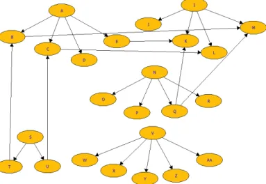
Fig. 2 presents the Bayesian network obtained from the EPB product line by applying the mapping rules presented in Section III.
Figure 2. DAG of the Bayesian network obtained from two physical alternative components of the Electric Parking Brake product line. Node were labeled using letters for the sake of spece. Interpretations are in tables 1 to 24
To complete our Bayesian network, we specify in tables 1 to 24 the prior probabilities of all root nodes and the conditional probabilities of all non-root nodes. Every node has two states: yes or no, indicating that the corresponding node is selected or not as part of a product. The root nodes only need two probabilities to be assigned (yes or no), independently of any other node. Nodes having N fathers need 2N conditional probabilities to be assigned to. For example, Table 2 states that node B, which is child of A and T, has a probability of: 0.3 to be selected and a probability of 0.7 to not be selected when nodes A and T are selected; 0 to be selected when
5
node A is selected and node T is not selected; 0 to be selected when node A is not selected; and 1 to not be selected when node A is not selected.
Table 1. Probability distribution of node A (ArchitectureDesignAlternatives)
Yes 1
No 0
Table 2. Probability distribution of node B (PullerCable)
A Yes No
T Yes No Yes No Yes 0.3 0.0 0.0 0.0 No 0.7 1.0 1.0 1.0
Table 3. Probability distribution of node C (ElectricActuator)
A Yes No
U Yes No Yes No Yes 0.3 0.0 0.0 0.0 No 0.7 1.0 1.0 1.0
Table 4. Probability distribution of node D (CalipersWithIntegratedActuators) A Yes No
Yes 0.25 0.0 No 0.75 1.0
Table 5. Probability distribution of node E (TraditionalPB) A Yes No
Yes 0.4 0.0 No 0.6 1.0
Table 6. Probability distribution of node I (ForceDistributionAlternatives)
Yes 1
No 0
Table 7. Probability distribution of node J (FullEPB) I Yes No
Yes 0.7 0.0 No 0.3 1.0
Table 8. Probability distribution of node K (Downsized_and_ESP_dynamicBraking)
I Yes No
E Yes No Yes No
Q Yes No Yes No Yes No Yes No
Yes 0.0 0.0 0.1 0.0 0.0 0.0 0.0 0.0
No 1.0 1.0 0.9 1.0 1.0 1.0 1.0 1.0
Table 9. Probability distribution of node L (IntegratedDownsizedCalipers) I Yes No
C Yes No Yes No Yes 0.1 0.0 0.0 0.0 No 0.9 1.0 1.0 1.0
Table 10. Probability distribution of node M (Downsized...)
I Yes No
B Yes No Yes No
Q Yes No Yes No Yes No Yes No
Yes 0.1 0.0 0.0 0.0 0.0 0.0 0.0 0.0
No 0.9 1.0 1.0 1.0 1.0 1.0 1.0 1.0
Table 11. Probability distribution of node N (SoftwareAllocationDesignAlternatives)
Yes 1
No 0
Table 12. Probability distribution of node O (NoECU) N Yes No
Yes 0.35 0.0 No 0.65 1.0
Table 13. Probability distribution of node P (DedicatedECU) N Yes No
6
Yes 0.3 0.0 No 0.7 1.0
Table 14. Probability distribution of node Q (ESP_ECU) N Yes No
Yes 0.3 0.0 No 0.7 1.0
Table 15. Probability distribution of node R (SpecificCockPitECU) N Yes No
Yes 0.05 0.0 No 0.95 1.0
Table 16. Probability distribution of node S (ElectricActionComponents)
Yes 1
No 0
Table 17. Probability distribution of node T (DC_motor) S Yes No
Yes 0.5 0.0 No 0.5 1.0
Table 18. Probability distribution of node U (EActuator) S Yes No
Yes 0.5 0.0 No 0.5 1.0
Table 19. Probability distribution of node V (InputInformation)
Yes 0.6
No 0.4
Table 20. Probability distribution of node W (TiltSensor) V Yes No
Yes 0.9 0.0 No 0.1 1.0
Table 21. Probability distribution of node X (EffortSensor) V Yes No
Yes 0.3 0.0 No 0.7 1.0
Table 22. Probability distribution of node Y (ClutchPosition) V Yes No
Yes 0.7 0.0 No 0.3 1.0
Table 23. Probability distribution of node Z (DoorPosition) V Yes No
Yes 0.2 0.0 No 0.8 1.0
Table 24. Probability distribution of node AA (VSpeed) V Yes No
Yes 0.7 0.0 No 0.3 1.0
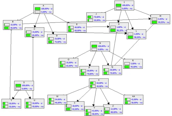
The Samiam2 tool was used to compute the prior probabilities of each node of the Bayesian network. A prior probability of a node represents the uncertainty about that node before receiving new information. Samiam uses the recursive conditioning algorithm to compute these probabilities. This algorithm recursively decomposes a network into two smaller sub-networks until the sub-networks only consist of a single probability distribution table. Then the algorithm uses these tables to compute the prior probabilities of each node. The resulting prior probabilities are presented in Fig. 3.
2 http://reasoning.cs.ucla.edu/samiam/
7
Figure 3. Prior probabilities of the Bayesian network corresponding to the EPB product line
The quantity of components needed in an hypothetical production plan scenario of 1000 cars per year, was computed using the (Ei = N * Ci * Pi) formula. The results, for each component of the EPB product line are presented in Table 25 below. Note that variation points are not taken into account in Table 25, as they do not correspond to physical components.
Table 25. Elements to compute the estimation of material needs for each variant of the EPB product line. Node of the Bayesian Network PriorProbability
(Pi) N° of instances (Ci) Estimation (Ei) B (PullerCable) 0.15 1 150 C (ElectricActuator) 0.15 2 300 D (CalipersWithIntegratedActuators) 0.25 2 500 E (TraditionalPB) 0.4 1 400 J (FullEPB) 0.7 1 700 K (Downsized_and_ESP_dynamicBraking) 0.018 1 18 L (IntegratedDownsizedCalipers) 0.015 2 30 M (Downsized...) 0.0045 1 4,5 O (NoECU) 0.35 1 350 P (DedicatedECU) 0.3 1 300 Q (ESP_ECU) 0.3 1 300 R (SpecificCockPitECU) 0.05 1 50 T (DC_motor) 0.5 1 500 U (EActuator) 0.5 2 1000 W (TiltSensor) 0.54 1 540 X (EffortSensor) 0.18 1 180 Y (ClutchPosition) 0.42 1 420 Z (DoorPosition) 0.12 0..2 Average=1 120 AA (VSpeed) 0.42 1 420 6. RELATED WORK
Zhang et al. [16] propose an approach based on Bayesian networks for assessing and predicting the quality of Software Product Lines (SPL). In their Bayesian network, nodes are variables representing design decisions and quality attributes. Design decisions are, for example, type-architecture (three-tier or distributed), type-system (Web or not Web), etc. Quality attributes are security, scalability and performance. In this approach, the Bayesian network is constructed by connecting characteristics to quality attributes. Then, experts assign conditional probabilities to each node in the network in order to quantify conceptual relationships. For example, a high probability can be assigned to node “scalability” if type-architecture is “distributed” and type-system is
8
“Web”, and a low probability is assigned to node “scalability”, if architecture is “three-tier” and type-system is “not Web”. This indicates that if this last configuration is chosen; probably the product will have low scalability. This approach helps to predict the software quality before constructing it.
Similarly, Kolesnikov et al. [6] propose a procedure for predicting quality attributes of all products of a SPL. This approach inferred product external attributes (e.g. behavior) from product internal attributes. Thus, data inferred from source code of a software product belonging to SLP, support predictions, for example about runtime behavior of software product, without executing them. Used data are obtained from software and network quality measures.
Larsson et al. [7] design a prediction-enabled component technology for PL architectures in the real-time systems domain. They provide a framework in which nonfunctional properties can be added to a component using analytical interfaces. These properties of the composed systems can be expressed and analyzed in relation to properties of built-in components. The aim of their work is to construct methods for predict these properties from predictable assembly of components.
Singh et al. [15] propose an approach to reliability analysis of component-based systems before they are built. This approach integrates a Bayesian analysis framework with Use Cases and Sequence Diagram. These models are annotated to incorporate information about expected system usage patterns and failure probabilities of the components. The annotated models are used for reliability prediction algorithm. This algorithm takes into account the estimation of reliability of components and their anticipated usage. This approach uses a Bayesian network to predict reliability of component-based systems.
Bencomo & Belaggoun [1] propose a Bayesian theory based approach for self-adaptive systems. But unlike our approach, they combine Bayesian networks are used with Decision networks, for solving real time decision problems.
7. CONCLUSION &OPEN ISSUES
This article presents an approach for the estimation of material needs for product lines. Starting from PLMs the approach generates Bayesian networks then analyses them. On the one hand, PLMs offer the benefit of early representation of variability in the product development cycle. On the other hand, the Bayesian approach is applicable in situations where past observations are scarce. While the PL approach is often applied in a software engineering context, in manufacturing industries it makes sense to couple PLM an Bayesian Networks for: (i) obtaining early estimations of the necessary amount of components for procurement when there is a large number of possible product configurations, and (ii) providing early insight on the reuse of components to support PL design decisions.
The approach was illustrated on a case study excerpt from the automotive industry – the EPB system. The main advantage shown with the case is that the approach is effective. However, the main issue that we encountered was the computation time of evaluation (exponential time for the general case). The approach is therefore probably not scalable. Still, as Bayesian networks are widely used, there is a great deal of research on efficient computation methods both for exact solutions, and approximation schemes.
Two important issues that are not addressed in this paper are precision and the downstream economic benefits. The first question is simple: “are the estimations safe?”. Empirical evidence is needed here. As for the second issue, many questions could be raised; how does this estimations technique benefits to industrials? How much does it cost when it fails? What are the other risks associated? Again further empirical investigation is needed.
REFERENCES
[1] Bencomo N., Belaggoun A. Requirements Engineering: Foundation for Software Quality. 19th REFSQ Working Conference, Essen-Germany, 2013.
[2] Clements P., Northrop L. Software Product Lines: Practices and Patterns, Addison-Wesley, Boston, 2001.
[3] De Lange F., Jansen T. The Philips-OpenTV product family architecture for interactive set-top boxes. In: Proceedings of the 4th International Product Family Engineering Workshop (PFE-4), Bilbao-Spain, 2001.
[4] Dumitrescu C., Mazo R., Salinesi C., Dauron A. Bridging the Gap Between Product Lines and Systems Engineering: An experience in Variability Management for Automotive Model-based Systems Engineering. 17th SPLC, Tokio-Japan, 2013. [5] Kang K., Cohen S., Hess J., Novak W., Peterson S. Feature- Oriented Domain Analysis (FODA) Feasibility Study, Technical Report
9
[6] Kolesnikov S. S., Apel S., Siegmund N., Sobernig S., Kästner Ch., Senkaya S. Predicting Quality Attributes of Software Product Lines Using Software and Network Measures and Sampling. In Proceedings of VaMoS. ACM New York, NY, USA, 2013.
[7] Larsson M., Wall A., Norstrom C., Crnkovic I. Using Prediction Enabled Technologies for Embedded Product Line Architectures. Proceedings of the Fifth ICSE Workshop on Component-Based Software Engineering: Benchmarks for Predictable Assembly, 2002. [8] Mazo R., Lopez-Herrejon R., Salinesi C., Diaz D., Egyed A. Conformance Checking with Constraint Logic Programming: The Case of
Feature Models. In 35th IEEE COMPSAC Conference, Munich-Germany, 2011.
[9] Mazo R., Salinesi C, Diaz D. Constraints: the Heart of Domain and Application Engineering in the Product Lines Engineering Strategy. International Journal of Information System Modeling and Design IJISMD. Sweden, 2011.
[10] Mazo R., Dumitrescu C., Salinesi C., Diaz D. Recommendation Heuristics for Improving Product Line Configuration Processes. To appear in: Recommendation Systems in Software Engineering. Robillard M, Maalej W., Walker R. and Zimmermann T. (Eds.). Springer. 2013.
[11] Pearl J. Probabilistic reasoning in intelligent systems: networks of plausible inference. Morgan Kaufmann. 1988.
[12] Pohl K, Bockle G, Linden FJvd. Software Product Line Engineering: Foundations, Principles and Techniques. Springer-Verlag New York, Inc., Secaucus, NJ, USA, 2005.
[13] Salinesi C., Mazo R., Diaz D., Djebbi O. Solving Integer Constraints in Reuse Based Requirements Engineering. 18th IEEE RE Conference. Sydney – Australia, 2010.
[14] Sharp D.C. Component Based Product Line Development of Avionics Software. In: SPLC, Denver, Kluwer, 2000.
[15] Singh H., Cortellessa V., Cukic B., Gunel E., Bharadwaj V. A Bayesian Approach to Reliability Prediction and Assessment of Component Based Systems. Proceedings of the 12th International Symposium on Software Reliability Engineering, 2001.
[16] Zhang H., Jarzabek S., and Yang B. Quality Prediction and Assessment for Product Lines. Lecture Notes in Computer Science Volume 2681, 2003.