HAL Id: hal-03134248
https://hal.archives-ouvertes.fr/hal-03134248
Preprint submitted on 8 Feb 2021
HAL is a multi-disciplinary open access
archive for the deposit and dissemination of sci-entific research documents, whether they are pub-lished or not. The documents may come from teaching and research institutions in France or abroad, or from public or private research centers.
L’archive ouverte pluridisciplinaire HAL, est destinée au dépôt et à la diffusion de documents scientifiques de niveau recherche, publiés ou non, émanant des établissements d’enseignement et de recherche français ou étrangers, des laboratoires publics ou privés.
Construction and update of an online ensemble score
involving linear discriminant analysis and logistic
regression
Benoît Lalloué, Jean-Marie Monnez, Eliane Albuisson
To cite this version:
Benoît Lalloué, Jean-Marie Monnez, Eliane Albuisson. Construction and update of an online ensemble score involving linear discriminant analysis and logistic regression. 2021. �hal-03134248�
1
Construction and update of an online ensemble score involving linear
discriminant analysis and logistic regression
Benoît Lalloué
a,b,*, Jean-Marie Monnez
a,b, Eliane Albuisson
c,d,eaUniversité de Lorraine, CNRS, Inria (Project-Team BIGS), IECL (Institut Elie Cartan de Lorraine), F-54000 Nancy, France; bInserm U1116, Centre d'Investigation Clinique
Plurithématique 1433, Université de Lorraine, Nancy, France ; c Université de Lorraine, CNRS, IECL (Institut Elie Cartan de Lorraine), Nancy, France; dDRCI CHRU Nancy, Nancy, France; e Faculté de Médecine, InSciDenS, Vandœuvre-lès-Nancy, France.
2
Construction and update of an online ensemble score involving linear
discriminant analysis and logistic regression
The present aim is to update, upon arrival of new learning data, the parameters of a score constructed with an ensemble method involving linear discriminant analysis and logistic regression in an online setting, without the need to store all of the previously obtained data. Poisson bootstrap and stochastic approximation processes were used with online
standardized data to avoid numerical explosions, the convergence of which has been established theoretically. This empirical convergence of online ensemble scores to a
reference “batch” score was studied on five different datasets from which data streams were simulated, comparing six different processes to construct the online scores. For each score, 50 replications using a total of 10N observations (N being the size of the dataset) were performed to assess the convergence and the stability of the method, computing the mean and standard deviation of a convergence criterion. A complementary study using 100N observations was also performed. All tested processes on all datasets converged after N iterations, except for one process on one dataset. The best processes were averaged processes using online standardized data and a piecewise constant step-size.
Keywords: Learning for big data, stochastic approximation, medicine, ensemble method, online score.
1 Introduction
When considering the problem of predicting the values of a dependent variable 𝑦, whether continuous (in the case of regression) or categorical (in the case of classification), from observed variables 𝑥1, . . . , 𝑥𝑝, which are themselves continuous or categorical, many different predictors can be constructed to addressthis problem. The principle of ensemble methods is to construct a set of “basic” individual predictors (using classical methods) whose predictions are then aggregated by average or by vote. Provided that the individual predictors are relatively good and sufficiently different from each other, ensemble methods generally yield more stable predictors than individual predictors [1].
3 This set of individual predictors can be constructed through different means, used separately or in combination, in order to obtain differences between them. Various types of regressions or rules of classification can be used as well as different samples (e.g. bootstrap), different variable selection methods (random, stepwise selection, shrinkage methods, etc.) or more generally by introducing a random element in the construction of predictors. Bagging [2], boosting [3], random forests [1] or Random Generalized Linear Models (RGLM) [4] are examples of ensemble methods. Another method for constructing an ensemble score in seven steps was recently proposed in Duarte et al. [5] and will be used as a reference in this article:
1. Selection of 𝑛1 classification rules.
2. Generation of 𝑛2 bootstrap samples which are the same as for the 𝑛1 rules.
3. Choice of 𝑛3 modalities of random selection of variables. For each bootstrap sample, selection of 𝑚 variables according to these modalities.
4. Selection of 𝑚∗ variables among 𝑚 by a classical method (stepwise, shrinkage, etc.). 5. For each classification rule, construction of the 𝑛2𝑛3 predictors corresponding to the
bootstrap sample and the selected variables.
6. For each classification rule, aggregation of predictors into an intermediate score. 7. Aggregation of the 𝑛1 intermediate scores from the previous step by averaging or vote.
Herein, we consider the case where y is a binary variable and the classification rules are linear discriminant analysis and logistic regression.
In a context of online data, i.e. a flow of data arriving continuously, one wishes to be able to update such an ensemble score when new data becomes available, without having to store all of the previously obtained data and performing the entire analysis. To achieve this goal, several stochastic
4 approximation processes which have been previously studied theoretically can be used together and will be detailed in Section 2.
However, the theoretical guarantees of convergence already demonstrated for this type of process provide little information on the practical choices to be made in order to obtain the best performances: e.g. “classical” or averaged processes, continuously decreasing step-size or not, etc. Therefore, to complete this study, Section 3 is dedicated to the empirical testing of this online score on several datasets, using several stochastic approximation processes for each classifier and comparing the accuracy of the estimations.
2 Theoretical construction and update of an online ensemble score
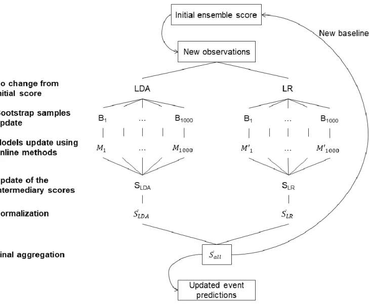
In order to be able to update online the ensemble score defined in [5] based on linear discriminant analysis and logistic regression, each bootstrap sample and each predictor must be updated when new data arrives [6]. Once the predictors are updated, the intermediate scores and the resulting final ensemble score are obtained using the same aggregation rules as for the offline ensemble method.
2.1 Updating the bootstrap samples
Starting from a sample size of 𝑛, the usual construction of a bootstrap sample consists in drawing at random with replacement n elements of the sample. In the case of a data stream, the Poisson bootstrap method proposed by Oza and Russell [7] can be used to update a bootstrap sample: for any new data, for each bootstrap sample 𝑏𝑖(𝑖 = 1, … , 𝑛2), a realization 𝑘𝑖 of a random variable under a Poisson law with parameter 1 is simulated, and the new data is added 𝑘𝑖 times to sample 𝑏𝑖. This new data can then be used to update the predictors defined using sample 𝑏𝑖.
5 2.2 Updating the predictors
Recursive stochastic approximation algorithms which take into account a mini-batch of new data at each step can be used to update the predictors. Such algorithms have been developed to estimate linear [8] or logistic [9] regression parameters, or to estimate the class centers in unsupervised classification [10] or the principal components of a factor analysis [11]. These algorithms do not require storing data and can, within a fixed timeframe, process more data than offline methods. Stochastic approximation algorithms able to update predictors obtained by linear discriminant analysis (LDA, equivalent to linear regression in the case of a binary dependent variable) and logistic regression (LR) are described below.
2.2.1 Updating logistic and linear regressions using a mini-batch of observations at each step
Note that all stochastic approximation algorithms described in this section use an online standardization of the data. Indeed, in practical applications, an inadequate choice of step-size of these processes or the presence of heterogeneous data or outliers can lead to numerical explosion issues in the non-asymptotic phase of the stochastic approximation process. To avoid numerical explosions in the presence of heterogeneous data, an online standardization of the data is proposed [8,9]; in the case of a data stream, the moments of the regression variables are a priori not known, but can be estimated online in order to perform the standardization. However, in this instance, the convergence of the stochastic approximation process is not ensured by classical theorems and was therefore proven in [8] in the case of linear regression, and in [9] in the case of logistic regression. Moreover, a too rapid decrease in step-size may reduce the speed of convergence in the non-asymptotic phase of the process. For this reason, following [12], the use of a decreasing piecewise constant step-size has been tested in [9].
6 Consider first the case of logistic regression. Let 𝑆 be a random variable taking its values in {0,1} and 𝑅 = (𝑅1⋯ 𝑅𝑝 1)′ with 𝑅1, … , 𝑅𝑝 being random variables taking values in ℝ, 𝑚 = (𝐸[𝑅1] … 𝐸[𝑅𝑝]0)′, 𝑅𝑐 = 𝑅 − 𝑚, 𝜎𝑘 the standard deviation of 𝑅𝑘, 𝛤 the diagonal square matrix with diagonal elements 1
𝜎1, … ,
1
𝜎𝑝, 1, 𝑍 = 𝛤𝑅
𝑐 the standardized 𝑅 vector, 𝜃 (𝑝 + 1,1) the vector of
parameters and ℎ(𝑢) = 𝑒𝑢
1+𝑒𝑢. The vector 𝜃 is the unique solution of the system of equations
𝔼 [𝛻𝑥ln ( 1+𝑒𝑍′𝑥
𝑒𝑍′𝑥𝑆 )] = 0, and thus of
𝔼[𝑍(ℎ(𝑍′𝑥) − 𝑆)] = 0. (1)
Let ((𝑅𝑛, 𝑆𝑛), 𝑛 ≥ 1) denote an i.i.d. sample of (𝑅, 𝑆) and for 𝑘 ∈ {1, … , 𝑝}, 𝑅𝑛𝑘 denote the average of the sample (𝑅1𝑘, … , 𝑅𝑛𝑘) of 𝑅𝑘 and (𝑉𝑛𝑘)2 =
1 𝑛∑ (𝑅𝑖 𝑘− 𝑅 𝑛 𝑘 ) 2 𝑛
𝑖=1 its variance (both computed
recursively), 𝑅𝑛 the vector (𝑅𝑛1⋯ 𝑅𝑛𝑝 0)′ and 𝛤𝑛 the diagonal matrix with diagonal elements 1
√𝑛−1𝑛 𝑉𝑛1
, … , 1 √𝑛−1𝑛 𝑉𝑛𝑝
, 1.
Assume that a mini-batch of 𝑚𝑛 new observatons (𝑅𝑖, 𝑆𝑖) constituting an i.i.d sample of (𝑅, 𝑆) is taken into account at step 𝑛. Denote 𝑀𝑛 = ∑𝑛𝑖=1𝑚𝑖 and 𝐼𝑛 = {𝑀𝑛−1+ 1, … , 𝑀𝑛}. Define for 𝑗 ∈ 𝐼𝑛, 𝑍̃𝑗 = 𝛤𝑀𝑛−1(𝑅𝑗− 𝑅𝑀𝑛−1) the vector 𝑅𝑗 standardized with respect to estimations of the means
and variances of the components of 𝑅 at step 𝑛 − 1. Recursively define the stochastic approximation process (𝑋𝑛, 𝑛 ≥ 1) and the averaged process (𝑋𝑛, 𝑛 ≥ 1):
𝑋𝑛+1= 𝑋𝑛− 𝑎𝑛 1
𝑚𝑛∑ 𝑍̃𝑗 𝑗∈𝐼𝑛
7 𝑋𝑛+1 = 1 𝑛 + 1∑ 𝑋𝑖 𝑛+1 𝑖=1 = 𝑋𝑛− 1 𝑛 + 1(𝑋𝑛− 𝑋𝑛+1). (3)
In the case of linear regression, the same type of process is used in [8] taking ℎ(𝑢) = 𝑢.
Assume:
(H1a) There is no affine relation between the components of 𝑅. (H1b) The moments of order 4 of 𝑅 exist.
(H2a) 𝑎𝑛 > 0, ∑∞𝑛=1𝑎𝑛 = ∞, ∑ 𝑎𝑛
√𝑛 ∞
𝑛=1 < ∞, ∑∞𝑛=1𝑎𝑛2 < ∞.
Theorem. Under H1a, H1b and H2a, (𝑋𝑛, 𝑛 ≥ 1) and (𝑋𝑛, 𝑛 ≥ 1) converge almost surely to 𝜃.
The proof of convergence is detailed in [8] in the case of linear regression and in [9] in the case of logistic regression. In these articles, these processes were compared to others (with or without online standardization, and with or without averaging) on real or simulated data. Empirical results showed the interest of using online standardization of the data to avoid numerical explosions as well as the better performance of averaged processes using a piecewise constant step-size (see Section 3).
2.2.2 Updating linear regression using all observations up to the current step
Recursively define the stochastic approximation processes (𝑋𝑛, 𝑛 ≥ 1) and (𝑋𝑛, 𝑛 ≥ 1):
𝑋𝑛+1 = 𝑋𝑛− 𝑎𝑛 1 𝑀𝑛∑ ∑ 𝑍̃𝑗 𝑗∈𝐼𝑖 𝑛 𝑖=1 (𝑍̃𝑗′𝑋𝑛− 𝑆𝑗), 𝑍̃𝑗 = 𝛤𝑀𝑛(𝑅𝑗− 𝑅𝑀𝑛) (4)
8 𝑋𝑛+1= 1 𝑛 + 1∑ 𝑋𝑖 𝑛+1 𝑖=1 = 𝑋𝑛− 1 𝑛 + 1(𝑋𝑛− 𝑋𝑛+1). (5) Note that 1 𝑀𝑛∑ ∑𝑗∈𝐼𝑖𝑍̃𝑗 𝑛 𝑖=1 𝑍̃𝑗′= 𝛤𝑀𝑛( 1 𝑀𝑛∑ ∑𝑗∈𝐼𝑖𝑅𝑗 𝑛 𝑖=1 𝑅𝑗′− 𝑅𝑀𝑛𝑅𝑀𝑛 ′ ) 𝛤𝑀𝑛 and 1 𝑀𝑛∑ ∑𝑗∈𝐼𝑖𝑍̃𝑗 𝑛 𝑖=1 𝑆𝑗 = 𝛤𝑀𝑛(1 𝑀𝑛∑ ∑𝑗∈𝐼𝑖𝑅𝑗 𝑛 𝑖=1 𝑆𝑗− 𝑅𝑀𝑛𝑆𝑀𝑛) 𝛤𝑀𝑛, 𝑆𝑀𝑛 = 1 𝑀𝑛∑ 𝑆𝑖 𝑀𝑛
𝑖=1 . Thus, the updating does not necessitate storing previous data since all empirical means and variances can be recursively computed. The same type of process would not be possible without storing the data for logistic regression, since in this case, 𝑍̃𝑗 in 𝑍̃𝑗ℎ(𝑍̃𝑗′𝑋𝑛) should be updated for all 𝑗.
Denote by 𝜆𝑚𝑎𝑥 the largest eigenvalue of the covariance matrix of 𝑅. Assume:
(H2b) (𝑎𝑛 = 𝑎 < 1
𝜆𝑚𝑎𝑥) or (𝑎𝑛 → 0, ∑ 𝑎𝑛
∞
1 = ∞).
Theorem. Under H1a, H1b and H2b, (𝑋𝑛, 𝑛 ≥ 1) and (𝑋𝑛, 𝑛 ≥ 1) converge almost surely to 𝜃.
This theorem was also proven in [8]. Empirical results again showed the interest of using online standardization of the data as well as all observations up to the current step to avoid numerical explosions and to increase the speed of convergence.
It is therefore possible to use the processes described in this section to update the predictors by linear discriminant analysis and logistic regression in the ensemble score, taking into account the sample of new data generated by the Poisson bootstrap at each step for each predictor.
9 3 Empirical study of convergence
3.1 Material and methods
3.1.1 Datasets
Four datasets available on the Internet and one dataset derived from the EPHESUS study [13] were used, all of which have previously been utilized to test the performance of stochastic approximation processes with online standardized data in the case of online linear regression [8] and online logistic regression [9]. The Twonorm, Ringnorm, Quantum and Adult datasets are commonly used to test classification methods. Twonorm and Ringnorm, introduced by Breiman [14], contain simulated data with homogeneous variables. Quantum contains observed “clean” data, without outliers and with most of its variables on a similar scale. Adult and HOSPHF30D contain observed data with outliers, as well as heterogeneous variables of different types and scales. A summary of these datasets is provided in Table 1.
Table 1. Description of the datasets
Dataset Na N pa p Source
Twonorm 7400 7400 20 20 www.cs.toronto.edu/~delve/data/datasets.html Ringnorm 7400 7400 20 20 www.cs.toronto.edu/~delve/data/datasets.html Quantum 50000 15798 78 12 derived from www.osmot.cs.cornell.edu/kddcup
Adult2 45222 45222 14 38 derived from www.cs.toronto.edu/~delve/data/datasets.html HOSPHF30D 21382 21382 29 13 derived from EPHESUS study
Na: number of available observations; N: number of selected observations; pa: number of available parameters; p: number of selected parameters.
The following preprocessing was performed on the data:
• Twonorm and Ringnorm: no preprocessing.
• Quantum: a stepwise variable selection (using AIC) was performed on the 6197 observations without any missing value. The dataset with complete observations for the 12 selected variables was used.
10 • Adult2: from the Adult dataset, modalities of several categorical variables were merged (in order to obtain a larger number of observations for each modality) and all categorical variables were then replaced by sets of binary variables, leading to a dataset with 38 variables.
• HOSPHF30D: 13 variables were selected using a stepwise selection.
From each dataset, a data stream was simulated step by step by randomly drawing, with replacement, 100 new observations at each step. Online scores were then constructed and updated from these data streams.
3.1.2 Reference batch score
For each dataset, a batch ensemble score was constructed using an adapted method from Duarte et al. [5] with the following parameters:
1. Two classification rules were used: linear discriminant analysis (LDA) and logistic regression (LR).
2. A total of 100 bootstrap samples were drawn for both rules (i.e. the same samples were used by each rule).
3. All available variables were included.
4. For each classification rule, the 100 associated predictors were aggregated by arithmetic mean and the coefficients subsequently normalized such that the score varied between 0 and 100 (as described in [5], Subsection 4.4.2) .
5. The aggregation between the two intermediate scores 𝑆𝐿𝐷𝐴 and 𝑆𝐿𝑅 was achieved by arithmetic mean: 𝑆 = 𝜆𝑆𝐿𝐷𝐴+ (1 − 𝜆)𝑆𝐿𝑅 with 𝜆 = 0.5.
11 The score obtained for each dataset was used as a “gold standard” to assess the convergence of the tested online processes (Figure 1).
12 3.1.3 Tested processes
Types of processes: Three different types of stochastic processes (𝑋𝑛) were used as defined below.
• “Classical” stochastic gradient (notation 𝐶_ _ _). At step 𝑛, card 𝐼𝑛 = 𝑚𝑛 observations (𝑅𝑗, 𝑆𝑗) were taken into account and the process was updated recursively: 𝑋𝑛+1 = 𝑋𝑛− 𝑎𝑛
1
𝑚𝑛∑𝑗∈𝐼𝑛𝑍̃𝑗(ℎ(𝑍̃𝑗
′𝑋
𝑛) − 𝑆𝑗), with 𝑍̃𝑗 the vector of standardized explanatory variables,
𝑆𝑗 ∈ {0,1}, ℎ(𝑢) = 𝑢 for the LDA, and ℎ(𝑢) = 𝑒𝑢
1+𝑒𝑢 for the LR.
• “Averaged” stochastic gradient (notation 𝐴_ _ _): 𝑋𝑛+1 = 1
𝑛+1∑ 𝑋𝑖 𝑛+1 𝑖=1 .
• Only in the case of the LDA: a process taking into account all of the previous observations (𝑅𝑗, 𝑆𝑗) at each step until the current step, 𝑗 ∈ 𝐼1∪ … ∪ 𝐼𝑛 (final mention “all”) [8]: 𝑋𝑛+1= 𝑋𝑛− 𝑎𝑛 1
𝑀𝑛
∑𝑛𝑖=1∑𝑗∈𝐼𝑖𝑍̃𝑗(𝑍̃𝑗′𝑋𝑛− 𝑆𝑗), 𝑍̃𝑗 = 𝛤𝑀𝑛(𝑅𝑗− 𝑅𝑀𝑛).
In all cases, the explanatory variables were standardized online (notation _𝑆 _ _): the principle and practicality of this method to avoid numerical explosions have already been shown [8,9]. Indeed, for some datasets (Adult2, HOSPHF30D), processes with raw data led to a numerical explosion, contrary to those with online standardized data.
Step-size choice: Tested step-sizes 𝑎𝑛 were either:
(i) continuously decreasing: 𝑎𝑛 = 𝑐 (𝑏 + 𝑛)⁄ 𝛼 (notation _ _ _𝑉);
13 (iii) piecewise constant [12]: 𝑎𝑛 = 𝑐 (𝑏 + ⌊
𝑛 𝜏⌋)
𝛼
⁄ (⌊. ⌋ being the integer part, 𝜏 the size of the level) (notation _ _ _𝑃).
In all cases, 𝛼 = 2/3 was taken as suggested by Xu [15] in the case of linear regression, 𝑏 = 1 and 𝑐 = 1.
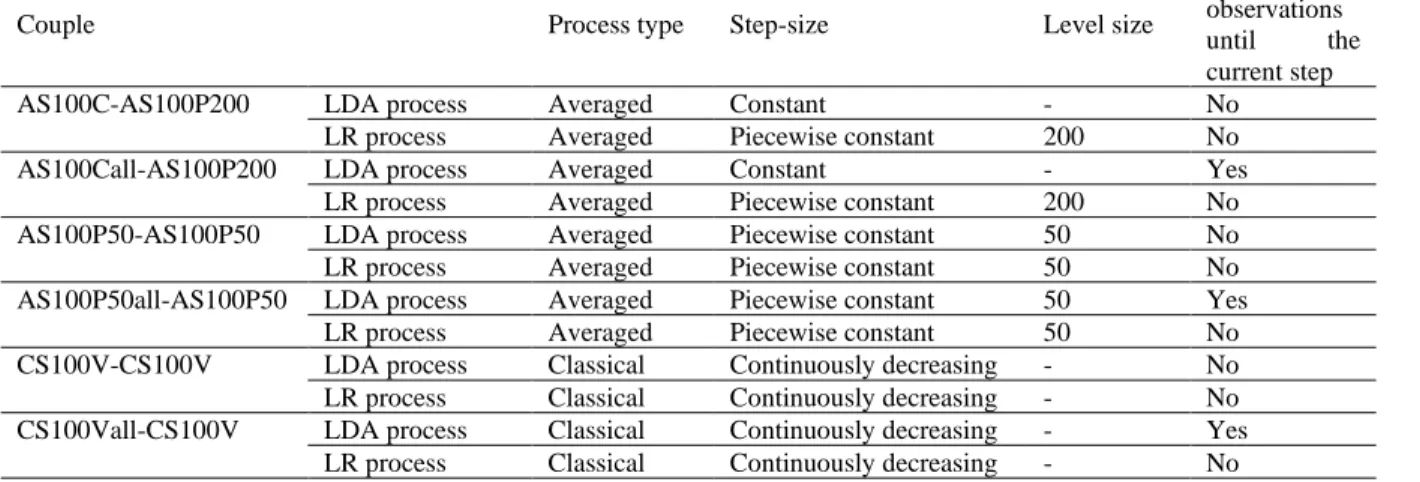
Tested processes: Six couples of processes were tested (Table 2). The latter were among those
which performed best in the studies published for online LDA [8] and for online LR [9], or represented “usual” processes frequently used (apart from online data standardization). A total of 100 new observations were used per step. Each process was applied to each of the streams generated from the datasets.
Table 2. List of the couples of processes studied
Couple Process type Step-size Level size
Use of all observations until the current step
AS100C-AS100P200 LDA process Averaged Constant - No
LR process Averaged Piecewise constant 200 No
AS100Call-AS100P200 LDA process Averaged Constant - Yes
LR process Averaged Piecewise constant 200 No
AS100P50-AS100P50 LDA process Averaged Piecewise constant 50 No
LR process Averaged Piecewise constant 50 No
AS100P50all-AS100P50 LDA process Averaged Piecewise constant 50 Yes
LR process Averaged Piecewise constant 50 No
CS100V-CS100V LDA process Classical Continuously decreasing - No
LR process Classical Continuously decreasing - No
CS100Vall-CS100V LDA process Classical Continuously decreasing - Yes
LR process Classical Continuously decreasing - No
All processes used online standardized data and 100 new observations per step.
In the notation describing a couple of processes, the first term is for the LDA and the second for the LR. For example, AS100Call-AS100P200 denotes the couple formed using an averaged process (A) for the LDA with online standardization of the data (S), 100 new observations per step (100), constant step-size (C) and taking into account all the observations up to the current step (all); and using an averaged process (A) for the LR with online standardization of the data (S), 100 new
14 observations per step (100) and a piecewise constant step-size with levels of size 200 (P200).
Note that the six couples of processes can be grouped in three pairs. In each pair, for the LDA part, one couple of processes uses 100 observations at each step and the other all observations up to the current step , the processes for the LR part being the same.
Convergence criterion: The convergence criterion used was the relative difference of the norms
∥𝜃𝑏−𝜃̂𝑁∥
∥𝜃𝑏∥ between the 𝜃
𝑏 vector of coefficients obtained for the batch score and the 𝜃̂
𝑁 vector of coefficients estimated by a process after 𝑁 iterations, the variables being standardized and the score being normalized to vary between 0 and 100 [5]. Convergence was considered to have occurred when the value of this criterion was less than the arbitrary threshold of 0.05. Three indicators were compared for each couple of processes: the criterion value for the synthetic score 𝑆𝐿𝐷𝐴 obtained by aggregating the LDAs, the criterion value for the synthetic score 𝑆𝐿𝑅 obtained by aggregating the LRs, and the criterion value for the final score 𝑆.
3.1.4 Convergence and stability analyses
In order to study the empirical convergence of the process, an analysis using a total of 10𝑁 observations was performed for each couple of processes. Since 100 observations are introduced at each step, the number of iterations of the process is N/10. Due to the stochastic nature of the processes studied, some variability is expected in the results. In order to evaluate this variability, the entire analysis using 10N observations was replicated 50 times for each couple of processes and for each dataset. The mean, standard deviation (SD) and relative standard deviation (RSD), i.e. the standard deviation divided by the mean, of the criterion values were studied for the intermediary and final scores. For each dataset, the average of the criterion values of all couples of
15 processes was also studied.
For each replication and each dataset, the performance of the couples of processes were ranked from the best (lowest relative difference of the norms for the final score 𝑆) to the worst (highest relative difference of the norms for 𝑆). Thereafter, the mean rank of each couple and its associated standard deviation over the 50 replications were computed, first by dataset, and finally over all datasets.
To study the long-term convergence of the process, a single analysis using 100𝑁 observations was performed for each couple of processes. Again, for each dataset, the values of the criterion for the intermediary and final scores were studied, and the couples of processes were ranked from the best to the worst. The mean rank over all datasets was used to compare the global performance of the couples. All analyses were performed with R 3.6.2.
3.2 Results
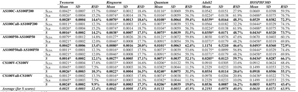
3.2.1 Convergence and stability analysis for 10𝑁 observations
When replicating each couple of processes 50 times, the mean criterion values were lower than 0.05 for all couples of processes applied on Twonorm, Ringnorm and Quantum datasets (Table 3). However, only three out of six couples of processes converged for Adult2 (AS100C-AS100P200, AS100P50all-AS100P50 and AS100Call-AS100P200) as well as for HOSPHF30D (AS100P50-AS100P50, AS100P50all-AS100P50 and AS100Call-AS100P200). Note that for Twonorm, Ringnorm and Quantum, the maximum criterion values (not shown) for all couples of processes were always lower than 0.05 (i.e. even the worst performing processes still converged), whereas it was not the case for certain couples applied on Adult2 and HOSPHF30D.
16 Table 3. Mean, standard deviation and relative standard deviation of the criterion after 50 replications
Twonorm Ringnorm Quantum Adult2 HOSPHF30D
Mean SD RSD Mean SD RSD Mean SD RSD Mean SD RSD Mean SD RSD
AS100C-AS100P200 SLDA 0.0042* 0.0007 15.7% 0.0066* 0.0012 18.4% 0.0116* 0.0069 59.8% 0.0542 0.0151 27.9% 0.0669 0.0398 59.5% SLR 0.0026* 0.0004 15.2% 0.0074* 0.0014 18.7% 0.0104* 0.0059 56.3% 0.0224* 0.0138 61.9% 0.0488* 0.0375 76.7% S 0.0028* 0.0004 14.6% 0.0070* 0.0013 18.6% 0.0108* 0.0064 59.4% 0.0339* 0.0164 48.3% 0.0529 0.0382 72.3% AS100Call-AS100P200 SLDA 0.0011* 0.0001 12.3% 0.0016* 0.0003 17.4% 0.0073* 0.0039 53.5% 0.0564 0.0182 32.2% 0.0444* 0.0329 74.1% SLR 0.0026* 0.0004 15.2% 0.0074* 0.0014 18.7% 0.0104* 0.0059 56.3% 0.0224* 0.0138 61.9% 0.0488* 0.0375 76.7% S 0.0016* 0.0002 14.2% 0.0038* 0.0007 17.5% 0.0075* 0.0039 51.5% 0.0350* 0.0171 48.7% 0.0434* 0.0320 73.7% AS100P50-AS100P50 SLDA 0.0079* 0.0012 14.8% 0.0127* 0.0026 20.1% 0.0121* 0.0072 59.8% 1.8030 0.8576 47.6% 0.0670 0.0403 60.1% SLR 0.0021* 0.0002 12.0% 0.0046* 0.0008 17.7% 0.0091* 0.0054 59.3% 0.0371* 0.0179 48.2% 0.0458* 0.0319 69.8% S 0.0042* 0.0006 13.4% 0.0080* 0.0016 20.0% 0.0101* 0.0063 62.4% 1.1174 0.5210 46.6% 0.0493* 0.0360 72.9% AS100P50all-AS100P50 SLDA 0.0011* 0.0001 12.3% 0.0016* 0.0003 17.5% 0.0073* 0.0039 53.6% 0.0175* 0.0099 56.8% 0.0444* 0.0329 74.4% SLR 0.0021* 0.0002 12.0% 0.0046* 0.0008 17.7% 0.0091* 0.0054 59.3% 0.0371* 0.0179 48.2% 0.0458* 0.0319 69.8% S 0.0014* 0.0002 12.1% 0.0027* 0.0005 17.1% 0.0071* 0.0037 52.1% 0.0205* 0.0123 59.7% 0.0434* 0.0287 66.1% CS100V-CS100V SLDA 0.0021* 0.0004 17.6% 0.0033* 0.0005 16.6% 0.0206* 0.0122 59.3% 0.0910 0.0305 33.6% 0.0912 0.0624 68.4% SLR 0.0045* 0.0003 7.5% 0.0016* 0.0003 16.3% 0.0382* 0.0044 11.5% 0.2329 0.0233 10.0% 0.1499 0.0353 23.5% S 0.0026* 0.0003 10.3% 0.0022* 0.0004 16.5% 0.0240* 0.0075 31.3% 0.0554 0.0114 20.6% 0.0918 0.0506 55.1% CS100Vall-CS100V SLDA 0.0012* 0.0002 13.3% 0.0016* 0.0003 17.8% 0.0074* 0.0038 51.4% 0.0978 0.0204 20.8% 0.0438* 0.0322 73.7% SLR 0.0045* 0.0003 7.5% 0.0016* 0.0003 16.3% 0.0382* 0.0044 11.5% 0.2329 0.0233 10.0% 0.1499 0.0353 23.5% S 0.0024* 0.0002 9.9% 0.0016* 0.0003 17.3% 0.0206* 0.0039 19.0% 0.0536 0.0087 16.2% 0.0855 0.0371 43.4%
Average (for S scores) 0.0025 0.0003 12.4% 0.0042 0.0008 17.8% 0.0133 0.0053 45.9% 0.2193 0.0978 40.0% 0.0610 0.0371 63.9%
* denotes criteria values < 0.05.
SD: standard deviation ; RSD: relative standard deviation
Table 4. Mean (SD) rank of the processes across the 50 replications, by dataset and overall (ordered by overall rank)
Dataset Twonorm Ringnorm Quantum Adult2 HOSPHF30D Overall
AS100P50all-AS100P50 1.04 (0.20) 3.00 (0.00) 1.68 (0.98) 1.40 (0.81) 2.54 (1.62) 1.93 (1.17) AS100Call-AS100P200 1.96 (0.20) 4.00 (0.00) 2.10 (0.84) 2.90 (1.15) 2.52 (1.27) 2.70 (1.12) CS100Vall-CS100V 3.40 (0.61) 1.06 (0.24) 5.24 (0.56) 4.08 (1.01) 4.60 (1.63) 3.68 (1.72) AS100C-AS100P200 4.42 (0.81) 5.06 (0.24) 3.64 (1.03) 2.56 (1.05) 3.56 (1.43) 3.85 (1.30) CS100V-CS100V 4.18 (0.66) 1.94 (0.24) 5.58 (0.70) 4.06 (0.98) 4.66 (1.62) 4.08 (1.53) AS100P50-AS100P50 6.00 (0.00) 5.94 (0.24) 2.76 (0.94) 6.00 (0.00) 3.12 (1.27) 4.76 (1.66)
17 Generally, intermediate LDA scores had smaller mean values, i.e. a faster convergence, than intermediate LR scores. However, the worst performing intermediary process was the LDA process AS100P50 applied on Adult2. In most cases, the mean criterion value for the final 𝑆 score was between those of the two intermediate scores 𝑆𝐿𝐷𝐴 and 𝑆𝐿𝑅. For some couples of processes applied on some datasets (for instance AS100Call-AS100C on Adult2 or AS100C-AS100P200 on HOSPHF30D), this led to a convergence towards the reference of the final score while one of the intermediate scores had not yet converged according to the criterion.
When studying the rankings of the couples of processes over the 50 replications, the best couple of processes overall was AS100P50all-AS100P50. This couple was consistently among the three best couples, and had the best performance for three datasets. Note that the three best couples of processes across all datasets were those using all observations until the current step for the LDA intermediary scores.
The observed differences in the average criterion were greater between datasets rather than between couples of processes (Table 4). Indeed, the means of each couple of processes were the lowest for Twonorm and Ringnorm compared to the other datasets. Conversely, all couples had their worst results for HOSPHF30D. Generally, all couples of processes performed better when applied on simulated data (Twonorm and Ringnorm) rather than on observed data (Quantum, Adult2, HOSPHF30D). This was also true when comparing the standard deviations and RSDs.
When comparing the overall variability of the rankings between the couples, AS100P50all-AS100P50 and AS100Call-AS100P200, the two best performing couples of processes on average, also had the lowest standard deviations for the mean overall rank (1.17 and 1.12 respectively), while the couple with the largest standard deviation was CS100Vall-CS100V (1.72).
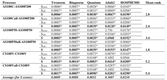
18 3.2.2 Convergence analysis for 100𝑁 observations
When studying the couples of processes after using 100𝑁 observations (i.e. N iterations) in order to assess the “long-term” convergence, the final online 𝑆 score was very similar (criterion value < 0.05) to the reference “batch” score for all of the couples on four of the five datasets tested (Table 5).
Only the AS100P50-AS100P50 couple applied to the Adult2 dataset did not converge after 100𝑁 iterations (criterion = 1.697). More precisely, the result for the LDA part of this couple differed substantially from its batch counterpart (criterion = 2.756), whereas the LR part appeared to converge to the batch LR part (criterion = 0.035).
Table 5. Criterion value after 100𝑁 observation used for intermediary and final scores
Processes Twonorm Ringnorm Quantum Adult2 HOSPHF30D Mean rank
AS100C-AS100P200 SLDA 0.0006* 0.0007* 0.0028* 0.0066* 0.0165* 2.8 SLR 0.0007* 0.0007* 0.0033* 0.0069* 0.0206* S 0.0006* 0.0007* 0.0030* 0.0067* 0.0190* AS100Call-AS100P200 SLDA 0.0006* 0.0007* 0.0046* 0.0153* 0.0060* 2.4 SLR 0.0007* 0.0007* 0.0033* 0.0069* 0.0206* S 0.0005* 0.0007* 0.0039* 0.0120* 0.0149* AS100P50-AS100P50 SLDA 0.0006* 0.0007* 0.0027* 2.756 0.0176* 3.4 SLR 0.0006* 0.0007* 0.0032* 0.0346* 0.0203* S 0.0005* 0.0007* 0.0029* 1.6968 0.0192* AS100P50all-AS100P50 SLDA 0.0006* 0.0007* 0.0046* 0.0100* 0.0060* 1.8 SLR 0.0006* 0.0007* 0.0032* 0.0346* 0.0203* S 0.0005* 0.0007* 0.0039* 0.0193* 0.0147* CS100V-CS100V SLDA 0.0010* 0.0020* 0.0073* 0.0076* 0.0165* 5.2 SLR 0.0033* 0.0009* 0.0168* 0.1002 0.0566 S 0.0015* 0.0014* 0.0083* 0.0414* 0.0289* CS100Vall-CS100V SLDA 0.0005* 0.0006* 0.0033* 0.0287* 0.0153* 5.4 SLR 0.0033* 0.0009* 0.0168* 0.1002 0.0566 S 0.0017* 0.0007* 0.0090* 0.0281* 0.0290*
Average (for S scores) 0.0009 0.0008 0.0052 0.3007 0.0210
* denote criteria values < 0.05.
First abbreviation: LDA process; Second abbreviation: LR process. Type of processes: C for classical SGD, A pour ASGD.
Data: R for raw data, S for online standardization of the data (1st number: number of new data per step). Step-size: V for continuously decreasing, C for constant, P for piecewise constant (2nd number: size of the steps of the piecewise constant step-size).
19 datasets, which consist of simulated data. The worst performances were obtained for Adult2 and HOSPHF30D datasets, which contain observed data.
Although these results are not directly comparable with the average results using 10𝑁 observations presented in the previous subsection (since there was only one replication using 100𝑁 observations), it should be noted that the criterion values of all couples of processes on all datasets were lower after 100𝑁 observations than the mean values after 10𝑁 observations, except for the LDA and global scores of AS100P50-AS100P50 applied on Adult2.
When the couples of processes were ranked from best to worst for each dataset and the average ranks were calculated across all datasets (Table 5), the two worst performing couples were CS100Vall-CS100V and CS100V-CS100V, i.e. the only two couples using classical processes and a continuously decreasing step-size. The best couple was again AS100P50all-AS100P50.
4 Conclusion
This study presented the constructing of an online ensemble score obtained by aggregation of two rules of classification, LDA and LR, and bagging. The online ensemble score was constructed by using Poisson bootstrap and by associating stochastic approximation processes with online standardized data of different types, averaged or not, using either a mini-batch of data at each step or all observations up to the current step in the case of LDA, and different choices of step-sizes, whose convergence has already been theoretically established. The convergence of this overall online score towards the “batch” score was studied empirically and the superiority of certain choices in the definition of the processes was observed, in particular the use of averaged processes and of a piecewise constant step-size. Other experiments could be carried out using randomly selected variables as opposed to all variables.
20
Acknowledgments
The authors thank Mr. Pierre Pothier for editing this manuscript.
Disclosure statement
No potential conflict of interest was reported by the authors.
Funding
This work was supported by the investments for the Future Program under grant ANR-15-RHU-0004.
References
[1] R. Genuer and J.-M. Poggi, Arbres CART et Forêts aléatoires, Importance et sélection de variables, preprint (2017). Available at https://hal.archives-ouvertes.fr/hal-01387654. [2] L. Breiman, Bagging predictors, Mach. Learn. 24 (1996), pp. 123–140.
[3] Y. Freund and R.E. Schapire, Experiments with a New Boosting Algorithm, in Proceedings of the Thirteenth International Conference on Machine Learning, 1996, pp. 148–156.
[4] L. Song, P. Langfelder and S. Horvath, Random generalized linear model: a highly accurate and interpretable ensemble predictor, BMC Bioinformatics 14 (2013), pp. 5.
[5] K. Duarte, J.-M. Monnez and E. Albuisson, Methodology for Constructing a Short-Term Event Risk Score in Heart Failure Patients, Appl. Math. 09 (2018), pp. 954–974.
[6] B. Lalloué, J.-M. Monnez and E. Albuisson, Actualisation en ligne d’un score d’ensemble, 51e Journées de Statistique, Nancy, France, 2019.
[7] N.C. Oza and S.J. Russell, Online Bagging and Boosting, in Proceedings of the Eighth International Workshop on Artificial Intelligence and Statistics, AISTATS 2001, Key West, Florida, USA, January 4-7, 2001, 2001.
[8] K. Duarte, J.-M. Monnez and E. Albuisson, Sequential linear regression with online standardized data, PLOS ONE 13 (2018), pp. e0191186.
[9] B. Lalloué, J.-M. Monnez and E. Albuisson, Streaming constrained binary logistic regression with online standardized data, J. Appl. Stat. (2021), pp. 1–21.
[10] H. Cardot, P. Cénac and J.-M. Monnez, A fast and recursive algorithm for clustering large datasets with k-medians, Comput. Stat. Data Anal. 56 (2012), pp. 1434–1449.
[11] J.-M. Monnez and A. Skiredj, Widening the scope of an eigenvector stochastic
approximation process and application to streaming PCA and related methods, J. Multivar. Anal. 182 (2021), pp. 104694.
[12] F. Bach, Adaptivity of averaged stochastic gradient descent to local strong convexity for logistic regression, J. Mach. Learn. Res. 15 (2014), pp. 595–627.
[13] B. Pitt, W. Remme, F. Zannad, J. Neaton, F. Martinez, B. Roniker et al., Eplerenone, a Selective Aldosterone Blocker, in Patients with Left Ventricular Dysfunction after Myocardial Infarction, N. Engl. J. Med. 348 (2003), pp. 1309–1321.
[14] L. Breiman, Bias, variance, and arcing classifiers, Tech. Rep. 460 Departement Stat. Univ. Calif. Berkeley (1996).
[15] W. Xu, Towards Optimal One Pass Large Scale Learning with Averaged Stochastic Gradient Descent, ArXiv11072490 Cs (2011).