Dynamics of Langmuir circulation in oceanic surface layers

Dynamics of Langmuir Circulation in

Oceanic Surface Layers

by

Anand Gnanadesikan A.B. Princeton University, 1988

Submitted in Partial Fulfillment of the Requirements for the Degree of

DOCTOR OF PHILOSOPHY at the

MASSACHUSETTS INSTITUTE OF TECHNOLOGY and the

WOODS HOLE OCEANOGRAPHIC INSTITUTION September, 1994

@Anand Gnanadesikan

The author hereby grants to MIT and WHOI permission to reproduce and distribute copies of this thesis document in whole or in part Signature of Author

Joint Program in Physical Oceanography Massachusetts Institute of Technology/ Woods Hole

Oceanographic Institution Certified by

A

,

r

I

Chairman, Joint Committee fdr Physical Oceanography, Massachusetts Institute of Technology/ Woods Hole

MASSACHUSETTS INSTITUTE Oceanographic Institution OF Tfr-4m nrY REl

UT

RISnc:

DYNAMICS OF LANGMUIR CIRCULATION IN OCEANIC SURFACE LAYERS

by

ANAND GNANADESIKAN

Submitted to the Joint Program in Physical Oceanography in partial fulfillment of the requirements for the Degree of

Doctor of Philosophy in Oceanography ABSTRACT

This work investigates whether large-scale coherent vortex structures driven by wave-current interaction (Langmuir circulation) are responsible for maintaining the oceanic mixed layer. Langmuir circulations dominate the near-surface vertical transport of momentum and density when the characteristic scale for forcing (defined as the Craik-Leibovich instability parameter YcLs) is stronger than the characteristic scale for diffusive decay Ydiff. Since the wave-current forcing is concentrated near the surface both terms depend on the cell geometry. Cells with long wavelengths penetrate more deeply into the water column. These cells grow more slowly than the fastest growing mode for most cases, but always dominate the solution in the absence of Coriolis forces. In the presence of Coriolis forces, the horizontal wavelength and thus the depth of penetration are limited. When a cell geometry is found such that 'YcLs >>diff, the current profile produced by small-scale diffusion is unstable to Langmuir cells and the cells replace small-small-scale diffusion as the dominant vertical transport mechanism for momentum and density. The perturbation crosscell shear is predicted to scale as YCLS. Such a scaling is observed during two field experiments. The observed velocity profile during these experiments is more sheared than predicted by a model which implicitly assumes instantaneous mixing by large eddies, but less sheared than predicted by a model which assumes small-scale mixing by near-isotropic turbulence. The latter profile is unstable to Langmuir cells when waves are present. The inclusion of cells driven by wave-current interaction explains the failure of the mixed layer to restratify on two days with high waves and low wind. Wave-current interaction introduces a small but efficient source of energy for transporting density which goes as the surface stress times the Stokes drift. Thesis Supervisor: Robert A. Weller

Title: Senior Scientist, Department of Physical Oceanography, Woods Hole Oceanographic Institution

Acknowledgments

While the errors and shortcomings of this work are my own, such strengths as may be found within it owe much to others.

My advisor Bob Weller played a huge role in this thesis. Much of our current knowledge of Langmuir cells is due to his persistence over the last two decades in pushing for accurate instrumentation with which to measure them, making the case time and again to funding agencies and the scientific community. Bob offered me the freedom to approach this rich and challenging problem in my own way, while providing tremendous resources and opportunities. He taught me the importance of grounding theoretical work in data, not simply assuming that the ocean behaves in a mathematically convenient way. He also was instrumental in teaching me to think scientifically.

Each member of my committee contributed to this document. Joe Pedlosky provided numerous ideas, comments, and suggestions for improving the

theoretical chapters. His insistence on consistency and rigor has greatly improved this work. Paola Rizzoli's detailed comments on early drafts were instrumental in helping me to define critical ideas, and her encouragement was also important at critical times. Paola has the gift of being able to give criticism without making the recipient feel stupid. Dave Chapman was instrumental in getting me started on the numerical modelling portions of the thesis. Gene Terray was always a good

sounding board for wacky ideas, and helped me formulate ideas about wave-current interaction and numerical modelling at a number of points. Al

Plueddemann was consistently encouraging, and helped greatly in defining the issues for the data chapters.

A number of other scientists deserve special mention. Jim Price was a wonderful chairman of my defense, conscientous and thorough. Chris Garrett helped me in the early stages of my work to clarify the important questions.

The two datasets which I used were the result of a great deal of hard work by a large number of people. Jerry Dean, Erika Francis, Melora Park-Samelson, Rick Trask, and Bryan Way played especially critical roles in generating these data sets, as did the crew of the Research Platform FLIP. I would also like to thank those who shared data with me, in particular Jerry Smith and Rolf Lueck.

The Office of Naval Research supported me throughout graduate school, first as an ONR Graduate Fellow- and later as a research assistant under the Surface Waves Processes Program (ONR Grant N00014-90-J-1495).

My deep thanks to friends, both from school and church, and family whose

love and support helped me through graduate school. Special thanks are due to my wife Amalia. Her love, confidence, and support have kept me going. She also put long hours in editing this thesis, making innumerable suggestions to improve clarity and style, as well as laying out figure, proofreading, and just asking me questions and making me explain just what I was trying to say.

They that go down to the sea in ships, that do business in great waters. These see the works of the Lord, and his wonders in the deep.

Oh that men would praise the Lord for his goodness, and for his wonderful works to the children of men!

Table of Contents

Abstract ... 3

Acknowledgments ... 5

Table of Contents ... 7

Chapter 1: Langmuir Circulation in the Oceanic Surface Layer ... 9

Chapter 2: The Instability of Langmuir Cells in Fluid Layers with No Coriolis Forces ... 22

Chapter 3: Structure and Instability of an Ekman Spiral in the Presence of Surface Gravity Waves ... 50

Chapter 4: The Spatial Scale of Equilibrium Langmuir Circulations ... 92

Chapter 5: The Velocity and Density Structure of Fluid Layers with Finite-Amplitude Langmuir Circulations ... 129

Chapter 6: Langmuir Circulation during the Mixed Layer Dynamics Experiment ... 170

Chapter 7: Langmuir Circulation during the Surface Waves Processes Program ... 225

Chapter 8: Finite-Amplitude Langmuir Circulation during MILDEX and SWAPP ... 274

Chapter 9: Conclusions and Discussion ... 299

Appendix A: Derivation of Huang's Equations ... ... 310

Appendix B: The Spectral Instability Code ... 325

Appendix C: The Finite-Difference Code ... 331

Appendix D: Measurement Errors for Current Meters on FLIP... 332

Appendix E: Thruster Contamination during MILDEX ... 339

References ... 344

Chapter 1: Langmuir Circulation in the Oceanic Surface Layer

Oceanographers have long been aware that the uppermost layer of oceans and lakes is relatively well mixed in contrast with the strongly stratified main thermocline lying directly below it. In the ocean this surface layer is home to the majority of primary production and the site of almost all oceanic photochemistry. It connects the atmosphere and the deep ocean and is involved in a vast number of biological, physical, and chemical processes of interest to oceanographers.

At many times, the upper portion of the surface layer is well-mixed with respect to conservative scalar quantities like temperature and salinity. This mixed

layer is not, however, well-mixed with respect to velocity. Figure 1.1a shows typical one-hour average profiles of velocity and temperature within the surface layer. The data shown were taken off the Research Platform FLIP in 1983. While

the temperature varies less than 0.01 degrees down to 40 meters, it is hard to determine the mixed layer base from the velocity measurements. The mixed layer

also contains relatively large time-varying shears. Figure 1.lb shows a one-hour time series of the velocity difference between 4.5m and 6.75m in an unstratified mixed layer. The data were also taken off FLIP. The data were band-passed for periods between 100 and 10000 seconds to eliminate the effect of surface gravity waves and inertial oscillations and subsampled to one sample per minute. There are velocity differences of several cm/s within the layer which display noticeable variability over time.

There are at present two views of how the mixed layer is maintained. One view (exemplified by the work of Mellor and Yamada, 1974; Klein and Coste,

1984) holds that the processes responsible have small spatial scales in comparison with the layer depth. The trajectory of a particle within the mixed layer is a

random walk as it is passed from one small eddy to another. Models based on this view parameterize mixing in terms of a small-scale eddy viscosity and produce horizontally averaged velocity profiles with a great deal of shear within a relatively isothermal mixed layer. The other view (exemplified by the work of Davis et al., 1981; Price et al., 1986) holds that motions with vertical and horizontal scales comparable to the mixed layer are responsible for its

E-W Velocity -20 -10 0 Velocity in cm/s -20 -10 0 Velocity in cm/s

(a)

(b)

Figure 1.1: Velocity Structure within oceanic mixed layers. (a) Hourly-averaged profiles of velocity in the east (left panel), and north (central panel) direction and temperature (right panel). Profiles are averaged from 1100-1200 local time on November 9th, 1983 off of R/P FLIP. (b) Stick plot of the velocity difference between 4.5 and 6.75m. Velocity data was collected at 0.5 Hz, band-passed for frequencies in the 0.01-0.0001 Hz band and subsampled to once per minute. Start time is 0000Z on March 5th, 1990. 10 I-0) 0) 0) N-S Velocity

the mixed layer is a slab within which the horizontally-averaged velocity is

completely homogenized. In the real world, however, there are persistent velocity differences within the mixed layer (as seen in Figure 1.1).

This thesis focuses on a mixing process involving eddies with spatial scales comparable to the mixed layer depth, the two-dimensional roll vortices known as Langmuir circulation or Langmuir cells. The following questions are asked: *Under what conditions do Langmuir cells replace small-scale mixing as the principal mechanism by which the mixed layer is stirred?

*When do Langmuir cells produce large spatially and temporally-varying velocity shears within the mixed layer?

*How do the cells affect the energy balance of the mixed layer?

In order to answer these questions certain subsidiary issues must be addressed: *When are Langmuir cells present in the mixed layer?

*What is the spatial structure of the cells? *What is the equilibrium population of cells?

Before plunging into the strategies which are used to answer these questions, some observational studies of Langmuir circulation are considered. These studies demonstrate that the cells are of the appropriate scale to affect the dynamics of the mixed layer.

1.2. Observations of Langmuir Cells

Langmuir (1938) was the first to make quantitative observations of the circulations which bear his name. Motivated by personal observations from an

ocean liner of rows of seaweed and debris lined up with the wind, he established many of the major features of the cells in an ingenious series of experiments on Lake George. Figure 1.2 shows a schematic of Langmuir circulation, illustrating

some of the major features established by Langmuir and subsequent investigators. The circulation involves roll vortices whose axes are horizontal and oriented at an angle x relative to the wind. The vortices have width Lcen/2. The typical velocities associated with these rolls are denoted by U in the crosscell (x) direction and Wup and Wdown in the vertical (z).The vortices are in general asymmetric, with

downwelling velocities exceeding upwelling velocities. The downwelling zones are associated with jets of water of width Ljet and characteristic perturbation velocity Vjet moving in the alongcell (+y) direction. The depth of the cells is D.

Often, the cells are associated with a surface layer in which there is a large velocity shear. The characteristic velocity in this layer is denoted in Figure 1.2 by

Vsuf and the depth of this layer by Dsuf. Although the figure shows Dsf as being much smaller than the cell depth D, there are some published cases (e.g. Van

Straaten,1950) where the cells are embedded within the shear layer. Velocities within the shear layer are often of order 10 cm/s.

Wind oo surf jet s D surf D S up W jet L /2 x

cell

Figure 1.2: A schematic of Langmuir circulation illustrating the concepts found in

the text

Properties of the cells have been described in the literature as follows:

* Geometry: The cells vary much more slowly in the alongcell than in the crosscell direction. Estimates of the ratio of alongcell length to crosscell spacing Lcen range from 3-4 (Thorpe, 1993) to of order 100 (Kenney, 1977). Cell spacing scales as the depth of the fluid (Van Straaten,1950, for cells seen on a tidal flat) or as the mixed layer depth (Smith et al., 1987). Oa ranges from 0-20 degrees (Faller, 1964).

* Vertical Velocities: Early observations of vertical velocities were made in lakes or in relatively calm conditions fairly close to surface, and the velocities seen were roughly 1-4 cm/s in the downwelling regions, and about 1-2 cm/s in the upwelling regions (Langmuir, 1938; Gordon, 1970). Recent work in more strongly forced layers (Weller et al.,1985, Weller and Price, 1988, Zedel and Farmer, 1991) has demonstrated the existence of stronger vertical velocities of order 5-25 cm/s.

* Horizontal Velocities: Velocities associated with the downwind jets have been

1938; Harris and Lott, 1973; Kenney, 1977; Ryanzhin, 1983; Smith et al., 1987). Crosscell velocities have been less frequently measured, but estimates of their magnitude fall into the same general range.

* Occurrence: Cells are often seen in stormy conditions where the waves and wind

stress are large and where the surface is being cooled (Weller and Price,1988) but they have also been observed at wind speeds of 2-4 m/s (Owen, 1966; Scott, 1970; Kenney, 1977) when the stratification was stable (Faller and Woodcock,1964) and when the mixed layer was being heated (Kenney,1977).

* Associated Phenomena: A number of investigators (Langmuir, 1938; Woodcock, 1944; Sutcliffe et al., 1963) report that seaweed or other biological debris is swept into surface convergence zones. Thorpe (1984), Smith et al (1987), and Zedel and Farmer (1991) show that bubbles generated by breaking waves are swept into cell convergence zones, producing curtains of bubbles which can be detected with sonars.

The cells as presented above are of the right order of magnitude to cause strong vertical transports of momentum and large horizontal variability in the mixed layer transport. This can be demonstrated as follows. Consider the vertical transport of momentum. The vertical and alongwind velocities associated with the cells are correlated. Let the momentum flux carried by the cells be defined as

2

pua, The downward transport of momentum in the downwelling zone may be estimated as -pWdownVjet. The transport of momentum in the upwelling zone -pWupVup may be estimated by noting that Wdownu-et=Wup(Lceln-Ljet) and Vup= VjetLjet/(Lcen - Ljet) since Vup, Vjet, Wdown, and Wjet are all perturbations from the mean mixed layer velocity. Averaging over the width of the cell:

Lcen

(1-1) 2

1

U*La=1 v'w'dx - 2VjetWdownLjet/Lcell

If Vjet and Wdown are approximately 2 cm/s and Wup is of order 1 cm/s, then since

Lt 1 2

Ljet/Lcei=1/3, U2La is 1.3 cm2/s2. This corresponds to a the stress caused by a wind

of about 7.5 m/s -a fairly stiff breeze. Larger estimates for cell velocities yield larger estimates for momentum fluxes. Langmuir cells are of the right order of magnitude to transport momentum within the mixed layer.

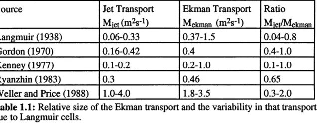
The variability in horizontal transport associated with Langmuir cells can also be large compared to the mean Ekman transport. We can estimate the amplitude of this variability by estimating the size of the transport relative to the base of the mixed layer carried in the jets. This "jet transport" Mjet is defined as

(1-2)i

(1-2) Mjet=Vjet*Djet'll

with these quantities are defined as in Figure 1.2. The Ekman transport (the total volume transport when the surface stress is wholly balanced by Coriolis force). is

(1-3) Mekman =P

where t is the surface stress, p the density and f the Coriolis force. Table 1.1 shows a comparison of these two quantities for several published observations of Langmuir cells. Mjet is often large compared with Mekman. This does not mean that the cells alter the value of the Ekman transport, but that the structure of this

transport is strongly influenced by the presence of cells. Once again Langmuir cells can determine the velocity structure within the mixed layer.

Source Jet Transport Ekman Transport Ratio

Miet (m2s-1) Mekman (m2s-1) Miet/Mekman

Langmuir (1938) 0.06-0.33 0.37-1.5 0.04-0.8

Gordon (1970) 0.16-0.42 0.4 0.4-1.0

Kenney (1977) 0.1-0.2 0.2-1.0 0.1-1.0

Ryanzhin (1983) 0.3 0.46 0.65

Weller and Price (1988) 1.0-4.0 1.8-3.5 0.3-2.0

Table 1.1: Relative size of the Ekman transport and the variability in that transport due to Langmuir cells.

1.3 Equations for mixed layer evolution and Langmuir circulation

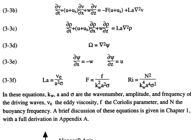
While Langmuir cells were long thought to play a critical role in upper ocean mixing, the dynamics of the instability process giving rise to the cells remained obscure for almost forty years. The situation was rectified in the 1970s by a series of papers (Craik, 1970; Craik and Leibovich, 1976; Leibovich,1977a,b; Huang,1979) which developed a set of equations for the evolution of a layer of fluid in the presence of surface gravity waves, stratification, Coriolis forces, and Langmuir cells. The equations are presented below as developed by Huang (1979).

DO DO D9 av av vs v ap

(1-4a) -- +(u+us)+w- = F( F-+ )+ + Ri-+LaV2Q2

(v

ap ap ap (1-4c) -+(u+us -+w-- = LaV2p (1-4d) Q = V2N (1-4e) ax = -w z =u ve f N2 (1-4f) La - F - Ri = kaa2o ka402 -1 (1-4g) k (x,y,z) = (x,y,z)

(1-4h) (kwa)20u,us,v,vs,w) = (u, us,, Vs, W)

(1-4i) 21 t=t

ka

_a

In the above equations, kw, a, and a are the wavenumber, amplitude and frequency of the driving surface gravity waves. Ve is the eddy viscosity, f the Coriolis

parameter, N the buoyancy frequency, and us and vs the Stokes Drift in the

crosscell (+x) and alongcell (+y) directions respectively. u and w are the horizontal and vertical velocities respectively in the crosscell (xz) plane. 2 and v are the vorticity and velocity respectively in the alongcell direction. Equations 1-4(a-e) are for dimensionless quantities, with equations 1-4(g-i) giving the conversion from dimensionless distance, velocity and time to dimensional (italicized) form. Equation (1-4f) defines three important dimensionless numbers. La is the

Langmuir number, which is a scaled eddy viscosity or inverse Reynolds number. F is a scaled Coriolis parameter. Ri is the Richardson number, the square of the ratio between a characteristic buoyancy frequency and a characteristic Stokes drift shear.

These equations are derived from a perturbation expansion (presented in full in Appendix A) in which the following scaling assumptions are made.

1. Cell velocities are small (of order E=kwa) in comparison with wave orbital velocities.

2. The cells evolve on time scales which are slow (order E2) in comparison with the wave frequency.

3. The cells are capable of carrying vertical fluxes of horizontal momentum of the same order as the surface stress La

Iz-o

4. The Coriolis force is of the right order to balance the surface stress.

5. The cells are capable of carrying density fluxes of the same order as the surface density flux Ll z=0'•

6. The turbulent eddy viscosity and eddy diffusivity are the same.

Bv

In combination, assumptions 3 and 4 mean that nonlinear terms wa must be of the same order as the Coriolis force terms and the diffusive terms.

In addition to the scaling assumptions, Huang's equations contain one other major assumption, that of a constant mixing coefficient. This is in many ways the weakest part of the equations. In the presence of wave breaking, for example, the mixing would be stronger near the surface, while in the presence of Kelvin-Helmholtz instability at the mixed layer base it would be stronger there. When interpreting results derived from these equations, the Langmuir number should be

thought of as setting the order of magnitude of the diffusive decay.

The approximation of constant mixing coefficient has a major effect on the density profile. In the absence of cells, the only possible steady-state solutions are those for which

a2p

(1-5) V2_{p = aZ}

2

-Thus the only possible solutions are those for which the density profile is constant or linear. In the absence of cells, the equations cannot support a solution with a thermocline and a mixed layer. Whether cells are present or not, at steady-state the density flux must be constant with depth. This is an unrealistic representation of mixed layer density evolution given that the time scales for mixing density through

the thermocline (which are of order weeks or months) are different from the time scales for adding heat to the mixed layer (of order hours or days).

The appearance of the Stokes drift in equations (1-4a,b) demands some extra explanation. The Stokes drift arises because irrotational surface gravity waves have larger alongwave velocities at the crest of the wave than at the trough. Averaging over a wave period, the mean velocity following a particle is nonzero, even though the mean Eulerian velocity at depths below the wave zone is zero (see Phillips, 1960 for a discussion). Given a monochromatic deep-water wave with wavenumber kw, frequency a, and amplitude a, the Stokes drift is

(1-6) vs(z)= kwa2a exp(2kwz)

This Lagrangian drift acts to tilt both planetary and relative vortex lines. In an Eulerian framework, this vortex interaction arises through nonlinear interactions

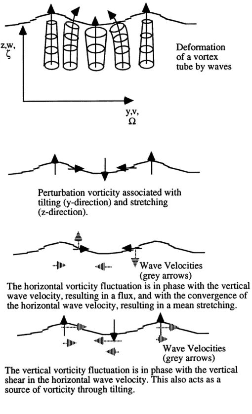
between the Eulerian-mean vorticity and the wave orbital velocity. Figure 1.3 illustrates these interactions for a vortex tube oriented in the +z direction for surface gravity waves propagating in the +y direction. In the presence of surface gravity waves, this tube is stretched at the wave crests, compressed at the wave trough and tilted in between. This means that vorticity perturbations in the y direction K' are created which are in phase with the vertical wave velocity w', and with the divergence of the horizontal wave velocity av'/ay. Likewise vorticity perturbations in the vertical direction z' are created in phase with the vertical shear associated the waves Dv'/Iz. As a result there are mean sources of vorticity FzQ'w',

l'Dv'/Dx , and CW'v'/)z where the overbar denotes averaging over a wave period. These terms go as the square of the wave velocity shear, which goes as the Stokes drift shear.

The research presented here differs from previous work in several ways. *It focuses on cases where the bottom boundary is a no-stress boundary. This is based on the observations (Weller ,1981; Price, Weller, and Schudlich, 1987)

showing that the momentum balance can generally be closed by integrating to the top of the main thermocline. (This is not true near the Coriolis frequency, but the propagation of inertial energy into the thermocline is beyond the scope of this thesis). In the majority of previous results, either the bottom boundary is a no-slip bottom (Lele, 1985), the stress on the bottom boundary is the same as at the top boundary, (Lele, 1985; Leibovich et al., 1989; Cox and Leibovich, 1993) or the water column is infinitely deep (Leibovich, 1977a).

*The mixing coefficients for density and velocity are the same. Previous authors (Leibovich and Paolucci, 1981; Lele,1985; Leibovich et al., 1989; Cox and Leibovich, 1993) considered cases where the turbulent Prandtl number (given by the ratio between the eddy viscosity and diffusivity) is equal to its molecular value of 7. This is not a good approximation for strongly turbulent mixed layers. Many mixed layer models assume a turbulent Prandtl number of 1 (Denman, 1973; Price et al. 1986) while others have it close to 1 (Mellor and Yamada, 1974). Setting the Prandtl number to be greater than one can lead to time-dependent solutions which are not necessarily realistic for oceanic cases.

*The effect of cells on the equilibrium profile when the surface forcing is balanced by small-scale mixing rather at the transient problem of how cells and small-scale mixing combine to establish a mixed layer is considered. The focus is on which process maintains the mixed layer rather than on how that layer is created.

z,w, Deformation

of a vortex

y,v,

Perturbation vorticity associated with tilting (y-direction) and stretching (z-direction).

•..jIII

"ll|-....

.

W ave Velocities

(grey arrows)

The horizontal vorticity fluctuation is in phase with the vertical

wave velocity, resulting in a flux, and with the convergence of

the horizontal wave velocity, resulting in a mean stretching.

.,, .. The vertical vorticity fluctuation is in shear in the horizontal wave velocity. source of vorticity through tilting.

Wave vlciuties

(grey arrows)

phase with the vertical

This also acts as a

Figure 1.3: Schematic of the production of horizontal vorticity by waves

interacting with a vertical vortex tube.

,;,,

...

-...

*The Stokes drift shear decays with depth rather than being a constant. Although some investigators (Leibovich, 1977a; Lele, 1985) have considered how the decay of the Stokes drift shear affects the instability problem, the effect on the structure of the cells at equilibrium has not been considered. When the Stokes drift and Eulerian shears within the mixed layer are nonuniform the dominant mode at equilibrium generally has a longer wavelength than the most unstable mode.

*The Coriolis force is nonzero. An implication of including Coriolis forces is that the Eulerian and Stokes drift shears will not necessarily be parallel and that the depth over which the cells penetrate is limited.

1.4 Langmuir Cells vs. Small Scale Mixing: The Plan of Attack

The equations introduced in the previous section are used over the course of this thesis to study when mixed layer profiles produced by small-scale mixing are unstable to cells, and to characterize the modification of these equilibrium profiles produced by finite-amplitude cells.

The fact that the forcing is concentrated near the surface of the layer makes for some difficulty. This may be seen more clearly by contrasting the problem at hand with the well-studied Rayleigh-Benard problem. For buoyant convection between two flat plates the strength of the the forcing is given by the buoyancy frequency N

(1-7) N =

where g is gravity, p is density and z is the vertical coordinate. The characteristic diffusive decay scale is given by

(1-8) Ydiff = NFvj(k242/D2)

where v is the viscosity, ic the diffusivity, k the horizontal wavenumber, and D the depth. If N>Ydiff one expects instability to occur and that the finite-amplitude cells will erase much of the initial stratification. For Langmuir cells, however, the Stokes drift decreases exponentially with depth scale k/2 (of order 10-20 meters). As a result it is unclear what the analogue of equation (1-7) should be. It is also unclear that the Craik-Leibovich instability mechanism will be able to force cells which can homogenize mixed layers with depths greater than k .

Chapters 2 and 3 attack the problem of defining analogues to the

stratification and Rayleigh number for Langmuir circulation. It is shown that for infinitesimal cells one can define the Craik-Leibovich instability parameter YCLS,

S0

0

0

(1-8) CL(D) F(z zd (z dz - (z z

where F(z) and G(z) are weighting functions which are proportional to the

nonlinear momentum and density fluxes carried by the infinitesimal cells. V and vs are the Eulerian velocity and Stokes drift, respectively, which are parallel to the cell axis. If Ydiff is a characteristic diffusive decay scale for the infinitesimal cells,

the stratified Craik-Leibovich Rayleigh number RaCLS is defined as:

(1-9) RaCLS-CLS/_ff

When RaCLS>1 (and additionally YcLS is greater than the frequency with which the cells are tilted by the crosscell shear), cells with a particular geometry are unstable. An important implication of this result is that YCLS and RaCLS depend on the vertical structure of the cells. Chapters 2 and 3 discuss how this vertical structure depends on the cell spacing, Langmuir number, Stokes drift profile, and boundary conditions. The cell spacing is particularly important,with long-wavelength cells penetrating deeper into the water column.

Since RaCLS depends on the spatial structure of the cells the question of which horizontal scales dominate the solution at equilibrium is important. Chapter 4 shows that in the absence of Coriolis forces, energy flows to the gravest modes.

This evolution is very slow once the cells reach some quasi-equilibrium mixed layer depth. Mathematically, stratification does not limit the depth of penetration of the cells, but the growth may be slow enough so that penetration is limited for geophysically interesting time scales. The presence of Coriolis forces acts to limit the horizontal length scale and thus the depth of penetration of the cells.

Suppose there is a cell geometry for which RaCLS ) 1 for infinitesimal cells. In Chapter 5 it is shown that at finite-amplitude, these Langmuir cells replace small scale eddy diffusion as the dominant means by which momentum and density are transported within the mixed layer. In such cases, the characteristic scale for shear within the mixed layer will go roughly as YCLS. The shear is a natural index of cell strength which can be used to isolate the forcing mechanism.

Chapters 6 and 7 use the framework developed in Chapters 2-5 to look at data from two experiments off the coast of southern California, the Mixed Layer Dynamics Experiment (MILDEX, Chapter 6) and the Surface Waves Processes Program (SWAPP, Chapter 7). The time-varying shear in a band from 1-36 cph is used as an index of cell strength. The level of this shear correlates extremely well

with an estimate of YCLS assuming cells of roughly 10m depth. These results represent the first prediction of cell strength in the field and support the idea that

the cells are driven by wave-current interaction. RacLS is shown to be large for extended periods of time, indicating that Langmuir cells rather than small-scale mixing should be the dominant mechanism by which the mixed layer is stirred. Comparisons between the observations and two one-dimensional mixing models further support this picture. When the cells are strong, the observed low-frequency (0.01-0.05 cph) shear profile has less shear within the mixed layer than predicted by a model which assumes small scale mixing, but more shear than predicted by a model which treats the mixed layer as a slab. The velocity profile which results from small-scale mixing unstable to Langmuir cells when waves are present. Additionally, both one-dimensional models predict restratification on two days during SWAPP when estimates of the energy balance of Langmuir cells

indicate that such restratification should not occur. In Chapter 8, finite-difference code runs demonstrate that the cells should indeed replace small-scale diffusion as the dominant transport mechanism within the mixed layer, homogenizing the velocity profile predicted by small-scale mixing. The result strongly supports the theses that cells are important in stirring the mixed layer and that wave-current interaction is important in driving the cells.

There are differences between theory and observations. Chapter 8 lists some of these shortcomings with respect to the predicted equilibrium cell population, mean shear and velocity structure, and total transport. Some possible remedies are

suggested. Chapter 9 concludes the thesis and suggests some avenues for future work.

1.5 Conclusions

This thesis argues that Langmuir circulations driven by wave-current interaction are the dominant mechanism for stirring strongly mixed oceanic

surface layers. When the surface forcing is strong, Langmuir cells are more important than small-scale diffusion driven by buoyant overturning and shear instability. In some cases, the cells are the reason why a mixed layer is seen at all. Although small-scale turbulent processes are potentially still important in the initiation of mixing (Chapter 9), as the mixed layer develops they become less important than large-scale Langmuir circulations.

Chapter 2: The Instability of Langmuir Cells in Fluid Layers

with No Coriolis Forces

2.1 Introduction

This thesis argues that Langmuir circulation driven by wave-current interaction, rather than small-scale diffusion driven by shear instability and local buoyant overturning, is primarily responsible for maintaining the mixed layer. In Chapter 1, a set of equations were introduced for the evolution of a layer of fluid in the presence of waves, Coriolis force, and Langmuir circulation. This chapter uses these equations to answer the following questions.

* Under what circumstances is the equilibrium solution set up by small-scale

turbulent diffusion unstable to Langmuir cells?

* How do diffusion, stratification, Stokes drift profile, layer depth, and cell spacing affect the growth rate and vertical structure of the unstable modes?

* What is the effect of the boundary conditions for density on the growth rate and

structure of the unstable modes?

The cases examined assume that the Coriolis force is zero, the cell axis, waves, and Eulerian shear are parallel (us=O), and that the wind stress is balanced by a pressure gradient. The goal is to reduce the many different parameters to a few important numbers. These turn out to be:

* The stratified Craik-Leibovich instability parameter YcLs (a measure of the

strength of the vortex forcing due to wave-current interaction and buoyancy). * The stratified Craik-Leibovich Rayleigh number RaCLS (a measure of the strength of the forcing relative to the diffusive decay).

* The aspect ratio of the cells Dmax/L where Dmax is the depth at which the maximum vertical velocity occurs.

The results can be extended to provide a basis for understanding the dynamics of infinitesimal and finite-amplitude cells in the presence of Coriolis forces.

Before embarking on this study we briefly note related work. Leibovich (1977a) studied the instability of an undisturbed column of infinitely deep water. He found that the growth rate of Langmuir cells was a strong function both of the Langmuir number and the horizontal wavenumber. Leibovich (1977b) showed that the maximum inviscid growth rate for cells in the presence of stratification was:

(2-1) y=max ( ~a) v N2

so that high stratification suppressed the instability. Lele (1985) showed that the marginal instability for Langmuir cells occurred at infinite cell spacing (k--O) when the bottom boundary was a no-stress bottom. Cox and Leibovich (1993)

considered the effect of changing this boundary condition on the instability.

This study uses a different initial condition from Leibovich (1977a), namely the equilibrium flow set up by small-scale diffusion in the absence of Langmuir cells. This initial condition was chosen since the goal of the thesis is to determine whether Langmuir cells or small-scale diffusion is the dominant transport

mechanism in an equilibrium mixed layer. This initial condition is not wholly unrealistic, since in real oceans and lakes there is almost always some pre-existing shear as a result of pressure gradients, internal waves, or inertial oscillations. As noted in Chapter 1, an additional difference between this work and that of previous investigators is that the turbulent Prandtl number is set equal to 1 instead of its molecular value of 7.

2.2 Equations of Motion and Methods of Solution

The equations of motion are (Leibovich,1977a)

DO Do

an avsav

Dp

(2-2a)

+u+w- = z Dx+RiD

Q

av v v lp+LaV2v (2-2b) -+u+w = - pa y +LaV2 ap ap ap (2-2c) _{tVux+wz = LaV}2_p (2-2d) J2 = V24

(2-2e)

- - w

u

k~a

In these equations kw,a, and a are the wavenumber, amplitude, and frequency of the driving surface gravity waves, Ve isthe eddy viscosity, N is the buoyancy frequency, and vs is the Stokes Drift. The italicized quantities are dimensional, with equations (2-2g-i) giving the conversion to nondimensional units. The key nondimensional numbers are the Langmuir number La and the Richardson number Ri. The boundary conditions on the velocity are

(2-3a) L- z=0=

(2-3b)

LavI

zz=.D=

z_

=

'z=-D

In the absence of Langmuir cells after a diffusive equilibrium is set up the mean Eulerian velocity in such a layer is given by

(2-4) ,,, (z+D)2

₁

(2-4)

V(z)-pLa 2D _{+(D pay t +C}

Where C is an undetermined constant which can be set equal to zero without altering the fundamental dynamics. In order to obtain a constant solution, the pressure gradient which is required to balance the wind stress is p/ay = t/D.

This scenario is not strictly realistic for the majority of oceanic cases, in which the primary balance is between wind stress and Coriolis force. However, it may be applicable to the flow in the interior of lakes where the spacing between convergence zones is small compared with the distance across the lake.

Additionally, as shown in Chapter 5, some results for mixed layers without

Coriolis force can be applied to mixed layers with Coriolis force when the Ekman depth

/- e

The density equation deserves some special consideration. As noted in the previous chapter, the mixing parameterization adopted for this study requires either that p be constant throughout the layer, or that it vary linearly from top to bottom. In both cases the density flux is constant throughout the layer. Since the deep ocean may be thought of as a reservoir of cold, dense water, the density is held fixed on the lower boundary.

(2-5) plz=-D = D

The upper boundary condition on density is less clear. The effect of two possible conditions are considered, one for which the density is fixed on the upper

boundary, and another for which the density flux is fixed on the upper boundary.

(2-6a) plz=o -0

If the density is fixed, the density flux carried by the cells is set by the internal

dynamics of the system, a somewhat more interesting case. However, it is unclear that it is a physical case, since the atmosphere is more likely to set the flux than it is to fix the density at the upper boundary.

In addition to the boundary conditions, there are a large number of

parameters which have a potential effect on the instability; namely the cell spacing L, layer depth D, Langmuir number La, Richardson number Ri, surface shear

av~z,

which must be considered, it is useful to choose parameter ranges which are reasonable for oceanic environments. For oceanic cases, the frequency of the driving waves is of order 0.5-1 rad/s, corresponding to periods of order 6-12

seconds. The e-folding depth for wave velocity decay 1/kw for such waves is roughly 8-32 meters. This thesis concentrates on layers with nondimensional

depths ranging from 2 to 6, corresponding to layer depths of about 15-200 meters. Reasonable values for oceanic eddy viscosities range from 10-1000 cm2/s

(Huang,1979; Weller,1981). Depending on how one calculates the quantity a2a (either by integrating over a spectrum or simply choosing values from the spectral peak) one may obtain a range of Langmuir numbers from O(10-4) to 0(1).

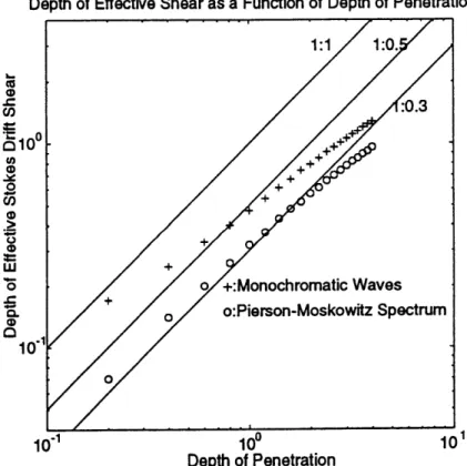
Two reasonable approximations for the nondimensional Stokes drift are used in this work, one for a monochromatic wave train and another for that given by the Pierson-Moskowitz spectrum (Pierson and Moskowitz, 1964):

(2-7a) vs(z)=exp(2z) Monochromatic

00

(2-7b) vs(z)= exp(-1.25 f )exp(2f2z)df P-M. Spectrum wheref is a dummy variable representing the nondimensional frequency. The Pierson-Moskowitz spectrum is chosen to have the same amplitude and peak frequency as the monochromatic wave train. Relative to the monochromatic wave train, the Pierson-Moskowitz spectrum yields a larger Stokes drift (by a factor of 4) and much larger Stokes drift shear (infinite at z-0) near the surface.*

The instability problem is cast as follows. The streamfunction, alongcell velocity, and Stokes drift are represented as

* _{Note that an infinite surface Stokes drift shear means that the inviscid limit on the growth rate (2-1) is}

always infinite and that a finite value of stratification will never act to limit the growth rate. This presents a major obstacle to applying the theory to the real ocean, and serves to motivate the development of an

(2-8a) y= Sy'(x,z,t)+(z)=eikx Nm(t)sin(--+

Tmsin(-m=1 m= 1

M M

(2-8b)

v=8v'(x,z,t)+V(z)=Seikx

vm(t)cos(Z)+

Vmcos(

)

m=O m=-O

M

(2-8c)

vs=

Vsmcos(Z

)

m=O

where

8

is a small number. Let the density field be

(2-9) p=p' (x,z,t)+P(z)=eikx m(t)sin(z+ sin(iPn

m=1 m=1

for density fixed on top and bottom boundaries or

(2-10) p=8eikx _{pn(t)cos( 2D ) mcos( 2D}

m=1 m=1

for density fixed on the bottom boundary and density flux fixed on the top

boundary. These expansions may be substituted into equations (2-2) and expanded in terms of 8. To zeroth order in 8 this procedure yields a Fourier-series

representation of the steady state solution in the absence of cells. At first order in

8, the growth rate of the linearly most unstable mode and the structure of that

mode can be cast as a linear eigenvalue problem in terms of the the coefficients Vm,vm,Pm. The value of the largest positive eigenvalue is a function of the number of modes in the truncation, but it converges as M becomes large. The results in this chapter are for M=40, a value for which all results presented here converged.

The vertical velocity for such an unstable mode is given by

M

(2-11) w=ik IVmsin(mCzl/D)eikx= ik ' m= 1

The depth at which the maximum vertical velocity occurs (Dm) is the depth at which IN'I is a maximum.

In section 2.3 a spectral instability code of the type outlined above is used to characterize the dependence of the growth rate and Dmax on layer depth, Stokes

drift shear profile, stratification, and boundary conditions. The growth rate and Dmax are closely linked.

In section 2.4 a simple understanding of these complicated dependencies is sought. Linearized energy balance equations for the instability are derived which give a sense of how quickly cells with a given shape grow. By making some simplifying assumptions, such as using two simple truncations to approximate the shape of the unstable modes, closed-form analytical solutions for the growth rate are obtained. These solutions are used to infer the important physical parameters which determine the growth rate and cell structure of the linearly unstable modes.

2.3 Craik-Leibovich Instability in Nonrotating Mixed Layers: Results from an

Instability Code

2.3.1 Results for Idealized Unstratified Surface Layers

This section focuses on two primary questions

1. How does the growth rate y of the linearly most unstable mode depend on the horizontal spacing of the cells L, the layer depth D, the Stokes drift profile, and the Langmuir number La?

2. How does the Dmax depend on these same parameters?

It is important to note the limitations of Dmax as an index of cell

penetration. Since the cell structure is not invariant it cannot be assumed that the

Structure of Streamfunction Perturbation Structure of Velocity Perturbation

0 00 + + + 0 + + -0.5 o0o o + -0.5 + .1 + + + 00o .1 + + -1 0 , -1 + + 4+ . + 1.5-1.5 +: La=0.001, L=2 +5 o: La=0.1., L16 0 _{- o:LaO. . E "16"} 0 0 0 0 -3. 000000 3. 0 0.5 1 0 0.5 1 (a) (b)

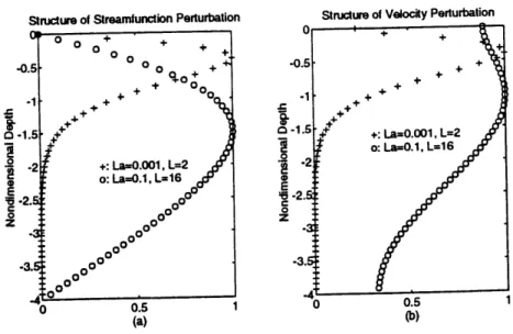
Figure 2.1: Vertical structure of the most unstable mode assuming monochromatic waves and a surface Eulerian shear of 1. (+) Langmuir number La--0.001, L=2. (o) La-0.1, L=16. (a) Streamfunction perturbation. (b) Velocity perturbation.

cells have no effect at depths more than twice Dma. Figure 2.1a shows the

streamfunction perturbation for the most unstable mode for La=0.001,k=2Rd2 (+) and La=0.1, k=27t/16 (o). Figure 2.1b shows the velocity perturbation. When La and L are small, the streamfunction perturbation is concentrated near the surface and resembles the velocity perturbation. When they are large, the streamfunction perturbation penetrates over the depth of the mixed layer and is very different from the velocity perturbation. Looking at Dma alone neglects these changes in

structure. Nonetheless Dm= is a useful diagnostic for cell penetration.

The linkage between growth rate and depth of penetration can be seen by considering a simple case. Suppose a monochromatic wave train is propagating in

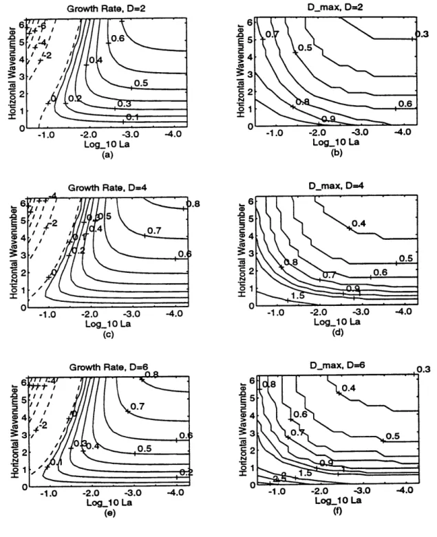
a direction parallel to the wind, so that the Stokes drift is given by (2-7a) and that the surface Eulerian shearz ' -z0=1. The maximum inviscid growth rate for this scenario is YCL =2. Figure 2.2a shows the growth rate of the most unstable mode y-=(L,N--O,La) and 2.2b the depth of the maximum vertical velocity

Dmax=Dmax(L,N-0,La) for a layer depth of 2. The horizontal axis is loglo La (1/La is analogous to Reynolds number), while the vertical axis is the horizontal

wavenumber k=27r/L. Dm, and y are linked as follows:

* Given a constant value of k, as La decreases y increases and Dmax decreases. * As La becomes very small, both y and Dm= asymptote to a constant value. * At very low values of La, large values of y occur when Dma is small.

This linkage is relatively insensitive to layer depth. Figure 2.2c and 2.2d show y and Dmx for a layer depth of 4, and 2.2e and 2.2f show y and Dma for a layer depth of 6. As La becomes small and k approaches 2n the growth rate of the unstable mode approaches 0.8, slightly more than half of Yc'' and Dmax is about 0.3 for all three values of depth. For larger wavenumbers, larger values of y

coupled to smaller values of Dmax are seen. For La= 10-5 _{the largest growth rate of}

1.19 occurs for cell spacing L=0.1 (k=20ft). Dmax for this unstable mode is 0.06. However, there are some parts of parameter space where the layer depth matters. In particular, at low wavenumbers and high La:

* Dmax is approximately half the layer depth.

* The stability boundary depends on the layer depth.

The importance of the layer depth for such cases is explained in Section 2.4. The effect of changing the Stokes drift profile from a monochromatic wave train to one corresponding to a Pierson-Moskowitz spectrum is shown in Figure

Growth Rate, D=2 Log_l0 La (a) Growth Rate, D=4 Log_l0 La (C) -2.0 -3.0 Log_10 La (e) -2.0 -3.0 Log_lO La (f)

Figure 2.2: Growth rate and depth of maximum vertical velocity Dma as a

function of horizontal wavenumber and Langmuir number given monochromatic

waves, no Coriolis force, and a surface Eulerian shear =1. Waves, wind and cell

axis are assumed collinear. (a) Growth rate, Layer depth D=2. (b) Dma, D=2. (c)

Growth rate, D=4. (d) Dma, D--=4. (e) Growth rate, D=6. (f) Dm,D=6.

Log_l 0 La (b) D_max, D=4 Log_l 0 La (d) Dmax, D=2

2.3. Figure 2.3a shows the Stokes drift for a Pierson-Moskowitz spectrum and 2.3b the Stokes drift shear. Using a wave spectrum rather than a monochromatic wave train increases the Stokes drift and Stokes drift shear for z>-1, decreases them for -1>z>-3 increases them for z<-3. Figure 2.3c shows y and 2.3d Dmax for a layer depth of 4 and a surface shear of 1 (corresponding to Figure 2.2c and d). The effect of changing the profile is to increase the growth rate for all values of horizontal wavenumber and Langmuir number, with the largest changes being at high

wavenumber and low Langmuir number. Dmax decreases fairly uniformly, with the mean decrease being close to 0.2. Increases in growth rate are correlated to

decreases in Dmax.

Lastly, the behavior of the instability at low wavenumbers is considered. Figure 2.4a shows the behavior of the growth rate of the most unstable mode for La=0.001 as k goes to zero for D=2,4, and 6 given a monochromatic wave train

and a surface Eulerian shear of 1.0. The growth rates decrease approximately quadratically, with marginal instability occurring at k=0 (infinite wavenumber). The growth rates are clearly strongly affected by the depth of the layer, with larger depths corresponding to larger growth rates. Figure 2.4b shows the depth of

penetration, which asymptotes to somewhat less than half the layer depth in all cases as the wavenumber k goes to zero.

In summary, the main results of the unstratified runs are:

* At high wavenumbers and low Langmuir numbers, the growth rate and depth of penetration are largely independent of layer depth and Langmuir number but

strongly dependent on cell spacing.

* At low wavenumbers, the growth rate depends on the value of La, the cell spacing and the layer depth.

* Changing the Stokes drift profile from one given by monochromatic waves to

one given by a Pierson-Moskowitz spectrum increases the growth rates sharply.

2.3.2 Instability in Idealized Stratified Mixed Layers

Turning now to stratified Craik-Leibovich instability, this section considers cases where D=4, the waves are monochromatic, and the surface shear=-l. From Leibovich (1977b) the maximum inviscid growth rate in the presence of

stratification is given by the maximum of - Ri. For the shear profiles in this chapter given a monochromatic wave train, the first product has a maximum

Stokes Drift -2 Solid: Pierson-Moskowitz Dashed: Monochromatic -3 Waves -4 0 1 2 3 4

Nondimensional Stokes Drift

(a)

Growth Rate, Pierson-Moskowitz

-1.0 -2.0 -3.0 -4.0 Log_l 0 La

(c)

Stokes Drift Shear

c -1 W ,- golid: Pierson-S- ' Moskowitz 0 Dashed: Monochromatic Z Waves -4 0.001 0.01 0.1 1 10 100 Nondimensional Stokes Drift Shear

(b)

D_max, Pierson-Moskowitz

-2.0 -3.0

Log_lO10 La

(d)

Figure 2.3: Effect on Craik-Leibovich instability of changing the waves from

monochromatic to a Moskowitz spectrum. (a) Stokes drift for Pierson-Moskowitz spectrum (solid)and monochromatic waves (dashed) with same peak frequency and amplitude. (b) Same as (a) but for Stokes Drift shear. (c) Growth rate from 40-mode instability code assuming Vo(z)=(z+D)2/2D, D=4 and waves given by a Pierson-Moskowitz spectrum. (d) Same as (c) but for depth of

maximum vertical velocity Dmax.

Growth Rate Dmax

103 10-2 Horizontal Wavenumber (a) E E 2 104 10-1 103 10-2 Horizontal Wavenumber

Figure 2.4: Growth rate and depth of maximum vertical velocity Dmax at low

wavenumber for three values of layer depth assuming monochromatic waves,

Vo(z)=(z+D)

/2D, and La=0.001. Solid lines are for D=2, dashed for D=4 and

chain-dotted for D=6. (a) Growth rate. (b) Dmax.

Solid: D=2 , Dashed: D=4

". Chain-dot: D=6

. *%.

of 2. The investigation is divided into cases where Ri<<2.0 (weak stratification), Ri somewhat smaller than 2.0 (moderate stratification) and Ri-2.0 (strong

stratification).

This section has two main purposes. The first is to investigate when the boundary conditions for density are important for determining the growth rate and

structure of the instability. This will guide the choice of a boundary condition for the finite-difference code runs in Chapters 4 and 5. The second purpose is to extend results from 2.3.1 to stratified cases to determine how the stratification affects the cell structure and growth rate.

Figure 2.5 shows growth rates and depth of cell penetration for cases of weak to moderate stratification. Figure 2.5a shows the growth rate and 2.5b Dmax for Ri=0.05 (weak stratification) with the density fixed on top and bottom

boundaries. Comparison with Figure 2.2c and d shows very little change in either the growth rate or the depth of maximum vertical velocity. Weak stratification does not affect the instability at high wavenumbers to any great degree.

Figure 2.5c and d repeat 2.5a and b for Ri-0.5 (moderate stratification). The growth rates decrease in the presence of moderate stratification, and D.m decreases as well. Given a fixed wavenumber, stratification can play a role in limiting the depth of penetration of the cells. Similar results were found by Lele (1985) and Li and Garrett (1993b).

Figure 2.5e and f repeat 2.5c and d, but for the density flux, rather than the density, fixed on the upper boundary. Changing the boundary condition produces very little difference in the growth rate or depth of maximum vertical velocity. Even for moderate values of stratification, the physics of the instability are relatively insensitive to the upper boundary condition.

This lack of sensitivity to boundary conditions does not hold when the stratification is strong. Figure 2.6a shows y and 2.6b Dmax as a function of wavenumber and La for Ri=2.0 and for density fixed on upper and lower

boundaries. In the absence of viscosity, there is no instability for Ri=2.0. This is not the case in the presence of viscosity. The growth rates have a very interesting pattern, showing a maximum in Langmuir number.

This pattern is strongly dependent on the upper boundary condition. Figure 2.6c and 2.6d show the growth rate and Dm for Ri=2.0 but with the density flux fixed on the upper boundary instead of the density. The instability is damped except at very low wavenumber and Langmuir number.

D_max, Ri=0.05 Density Fixed

Log_lO La (b)

D_max, Ri=0.5 Density Fixed

Log_l0 La (c) -2.0 -3.0 Log_lO10 La (e) -1.0 -2.0 -3.0 -4.0 Log_l 0 La (d) -1.0 -2.0 -3.0 -4.0 Log_lO La (f)

Figure 2.5: Instability of Langmuir cells in the presence of low to moderate

stratification. All cases assume layer depth D=4, monochromatic waves, no

Coriolis forces and a surface Eulerian shear of 1. (a) Growth Rate, Ri-0.05 density

fixed on both boundaries. (b) Dmax, Ri-0.05, density fixed on both boundaries.

(c) Same as (a), but for Ri=0.5. (d) Same as (b) but for Ri-0.5. (e) Same as (c) but

for density flux fixed on upper boundary.

(f)

Same as (d) but for density flux fixed

on upper boundary.

Growth Rate, Ri=2.0 Density Fixed III / > 4I 32 01 / 0 -1.0 Growth Rate, Log_l 0 La (a)

Ri=2.0, Density Flux Fixed

Log_10 La

(b)

D_max, Ri=2.0 Density Flux Fixed

I/ / , A2 -1.0 -2.0 -3.0 -4.0 Log_l 0 La (c) Growth Rate Solid:Ri=O Dashed:Ri=2,Density ied Chain-dot:Ri=2, Fixed 4 -2 10 10 2 Horizontal Wavenumber (e) E E2 '-co ,1 0. 0 1 4 10 101 El3 -10 10" Horizontal Wavenumber (f)

Figure 2.6: Instability of Langmuir cells at high values of stratification. All runs shown assume monochromatic waves, layer depth D=4, no Coriolis forces and a

surface Eulerian shear of 1.0. (a) Growth rate, Ri=2.0, density fixed on top and bottom boundaries. (b) Dmax, Ri=2.0, density fixed on top and bottom boundaries.

(c) Same as (a) but for density flux fixed on upper boundary. (d) Same as (b) but

for density flux fixed on upper boundary. (e) Growth rate at very low wave-number given La=0.001. Solid line is for Ri=0.0, dashed for Ri=2.0 with density fixed on both boundaries, chain-dotted for Ri=2.0 with density flux fixed on upper boundary. (f) Same as (e) but for Dma.

&6 (D 5' 2 0 01 0 Log_10 La (d) D_max c 10-2 10 , " 6 104 Solid:Ri=0 Dashed:Ri=2,Density Fixed Chain-dot:Ri=2,Flux Fixed -*- -I 0"

At low wavenumber and Langmuir number, there is some instability even when the stratification is strong. Figure 2.6e shows y and Figure 2.6f Dax for La=0.001, D=4, given a monochromatic wave train and a surface shear of 1.0. The solid line is for Ri=0.0. The dashed line is for Ri=2.0 with density fixed on the top and bottom boundaries. The chain-dotted line is for Ri=2.0 with the density fixed on the lower boundary and the density flux fixed on the top boundary. The growth rates are smaller for the two stratified cases and Dmax is smaller as well, indicating that the cells are trapped closer to the surface. The upper boundary condition is also important for the growth rates at low wavenumbers, with a flux boundary condition on the upper boundary giving lower growth rates. As the wavenumber becomes very small, both the growth rate and depth of maximum vertical velocity asymptote to the unstratified value.

The four major results for stratified Langmuir cells are thus

*At weak to moderate values of stratification, the growth rates and depth of maximum vertical velocity for the linearly unstable modes is not greatly affected

by the upper boundary condition and the overall pattern resembles that in the absence of stratification.

*Stratification reduces both the growth rate and depth at which the maximum vertical velocity occurs.

* For strong values of stratification, the value of La as well as the upper boundary

condition is critical in determining the growth rate and depth of maximum vertical velocity for the linearly unstable modes.

* At low wavenumbers, however, the stratified results asymptote to the unstratified results even for high values of stratification.

2.4 The Physics of Craik-Leibovich Instability 2.4.1 Energetics of the Instability

In order to understand the results of Section 2.3, we will now derive equations for the energy balance which demonstrate how the cell structure determines the growth rate, and how the Langmuir number, Stokes drift profile,

stratification, and boundary conditions determine the cell structure. Take the linearized equations of motion. As in Section 2.2 let 5'V,8v',8p' represent the perturbation streamfunction, velocity, and density fields, while 'o,V and Po represent the equilibrium fields in the absence of cells. Substituting into (2-2), the equations to zeroth order in 8 are:

(2-12b)

(2-12c)

while to first order in d: (2-13a) (2-13b) (2-13c) (z+D)2 Vo(z) - 2D Po(z) =- z

a

av~av'

t V2 = Z ax+ Ri

ap'

tav z

3x

LaV2_v'

ap' aPoAV

-t

a-

& LaV

p'

Multiplying equation (2-13a) by V', (2-13b) by v', (2-13c) by p', and designating horizontal averaging by an overbar gives the perturbation variance equations:

0

0

(2-14a

)

-~ ;V d

0

-

Ri

p'w'dz-

dz

a

----

,aVo

_{'vw dz}

_w -d

-0

0

+rz oz

Then the energy balance is (2-15a)

(2-15b)

(2-15c)

a

a- Ecc= Pstokes - Btrans - Ec

a

j Eac= Pac - Eac

SEp= Pp - ep

where Ecc,ac are the energies associated with flow in the crosscell and alongcell directions respectively. Ep is the density variance. Pstokes is the Stokes production (the work done by the waves on the cell vortices). Pac is the shear production. Pp is the density variance production. Btrans is the buoyancy transport. Ecc,ac,p are the dissipation terms associated with the crosscell velocities, alongcell velocity, and density respectively. Define v'=vle tV(z)cos(kx) p'=ple^fp(z)cos(kx)

(2-16a)

(2-16b)

-- +- dz

so that the perturbation structure of each field is given by a shape function

multiplied by an amplitude.The structure functions V, V,p are normalized so that:

0

(2-17) ~ I(V,yp)12dz =1

Substituting into the crosscell energy balance and letting y be the growth rate then yields the following relation between the three amplitudes

2(2-18) 0 (2 -1 8 ) --i Pa

_J7)

r2

La

Kz)p(z)dz

(2-19d)

and dividing out c (2-20) Similarly, by defil (2-21a) (2-21b) 4=

₂

I

D-j

:ommon terms, yields

4 2 2 2Ri y+ La K/k) , = kVsz/k vl + Ri k pl ning 0 A 2 1Vo VzD ipg(z)V(z dz ^2

POz

2

)t~~p(fa

dz

.s

0 0

2

2

2

La

(2-21c) k +k2_{V2 dz kP = D+k} 2_p2_dz

the equations for alongcell velocity and density may also be obtained

(2

(2-22a) 7y+ La k)vl = k VzVj

(2-22b)

(y+La k)pi =

k P Vl

Substituting into (2-20) and letting

(2-23a) ACL=AZVz

(2-23b) N2= Ri P1A0

yields the following, cubic equation for y

(2-24) (,y+ La K, ) (y + La k) (y+ La k)=

k2L/k7 + La k +k2N2/k ( + La k

By considering some simple solutions of equation (2-24) it is possible to

understand the physics behind the results of section 2.3. This is done during the remainder of this section.

2.4.2 Linking Cell Structure and Growth Rate at High Wavenumber

Suppose that the density and velocity perturbations have identical structure functions, so that V(z)=p(z), and kp=lk. Then the solution to (2-24) is

2 2

La (k + k /k )

(2-25) 7=- 2

La2 (

k

The stratified Craik-Leibovich instability parameter

YCLS

(2-26a) YCLS = TCLN 2

(2-26b) Ydiff= La

k

rWk

Then the necessary condition for instability is that

(2-27) RaCLS - LS >1

tdiff

(2-28) =

-

Equation (2-26a) may be squared and rewritten as follows

0

0

(2-29)

=

z)V(z

dzjiV(z)V(1zdz

-0

₀

Ri V!/z)p(Z zz dz (z)p(z) dz

Which may be rewritten in dimensional form as:

0

0

0

(2-30)4 a vV p

(2-30) LS(D) = F(z dz (z dz G(z dz

so that TCLS corresponds to the local instability parameter defined by Leibovich (1977b) and shown in (2-1), but with the various components defined by depth-averages rather than by local values. The weighting functions F(z) and G(z) used to define the depth-average depend on the shape of the momentum and density transport carried by the cells.

In order to get a better feel for the what the various terms mean, the streamfunction, density, and alongcell velocity structure functions may be approximated as follows

(2-31a) l/= sin(z/D') z > -D'

(2-31b) V,p = cos(icz/2D') z > -D'

(2-31c) V,V,p =0 z < -D'

so that D'=2Dmax. In this truncated representation of cell structure, the cells

penetrate over D', but have no effect below D'. This truncation will be denoted T1. Because the cell penetration depth is limited, Truncation T1 models cells which are not affected by the different bottom boundary conditions on velocity and density.

Defining YCLS1 as YCLS when the structure functions are given by Truncation T1, and noting that k=Ky- k24 2/D'2 then

(2-32a) Ydiff= La (k2+i2/D'2_{) k}2_+nr2_/4D'2_/k