HAL Id: hal-00317891
https://hal.archives-ouvertes.fr/hal-00317891
Submitted on 14 Oct 2005
HAL is a multi-disciplinary open access
archive for the deposit and dissemination of
sci-entific research documents, whether they are
pub-lished or not. The documents may come from
teaching and research institutions in France or
abroad, or from public or private research centers.
L’archive ouverte pluridisciplinaire HAL, est
destinée au dépôt et à la diffusion de documents
scientifiques de niveau recherche, publiés ou non,
émanant des établissements d’enseignement et de
recherche français ou étrangers, des laboratoires
publics ou privés.
time-varying magnetic reconnection: II. Measuring
expansions in the ionospheric flow response
S. K. Morley, M. Lockwood
To cite this version:
S. K. Morley, M. Lockwood. A numerical model of the ionospheric signatures of time-varying
mag-netic reconnection: II. Measuring expansions in the ionospheric flow response. Annales Geophysicae,
European Geosciences Union, 2005, 23 (7), pp.2501-2510. �hal-00317891�
Annales Geophysicae, 23, 2501–2510, 2005 SRef-ID: 1432-0576/ag/2005-23-2501 © European Geosciences Union 2005
Annales
Geophysicae
A numerical model of the ionospheric signatures of time-varying
magnetic reconnection: II. Measuring expansions in the ionospheric
flow response
S. K. Morley1,*and M. Lockwood1,2
1School of Physics and Astronomy, University of Southampton, UK 2Rutherford Appleton Laboratory, Chilton, Oxfordshire, UK
*now at: CRC for Satellite Systems, University of Newcastle, NSW, Australia
Received: 24 February 2005 – Revised: 6 June 2005 – Accepted: 30 June 2005 – Published: 14 October 2005
Abstract. A numerical model embodying the concepts of the Cowley-Lockwood (Cowley and Lockwood, 1992, 1997) paradigm has been used to produce a simple Cowley– Lockwood type expanding flow pattern and to calculate the resulting change in ion temperature. Cross-correlation, fixed threshold analysis and threshold relative to peak are used to determine the phase speed of the change in convection pat-tern, in response to a change in applied reconnection. Each of these methods fails to fully recover the expansion of the onset of the convection response that is inherent in the simu-lations. The results of this study indicate that any expansion of the convection pattern will be best observed in time-series data using a threshold which is a fixed fraction of the peak response. We show that these methods used to determine the expansion velocity can be used to discriminate between the two main models for the convection response to a change in reconnection.
Keywords. Magnetospheric physics (Magnetosphere-ionosphere interactions) – Ionosphere (Plasma convection; Modeling and forecasting)
1 Introduction
The nature of the ionospheric convection response to a change in the IMF is the subject of much discussion, with evidence for two apparently conflicting viewpoints. The pre-vailing views are 1) that the convection response first appears locally on the dayside before evolving around the flanks and into the nightside (Lockwood et al., 1986; Etemadi et al., 1988; Saunders et al., 1992; Khan and Cowley, 1999; Cowley and Lockwood, 1992, 1997) – henceforth referred to as the CL model, 2) that the convection response is globally
simul-Correspondence to: S. K. Morley
(steven.morley@newcastle.edu.au)
taneous (Ridley et al., 1998; Ruohoniemi and Baker, 1998; Ruohoniemi and Greenwald, 1998) – this will be referred to as the REA model.
Some recent papers have reported a two-stage ionospheric convection response (Murr and Hughes, 2001; Lu et al., 2002; Nishitani et al., 2002) to a change in the magneto-pause reconnection rate. These papers present observations that show that both quasi-instantaneous and expanding re-sponses can occur concurrently, however, no consensus has yet been reached on a mechanism that incorporates both re-sponses within a single framework. Further, modelling of the ionospheric convection response by Lockwood and Morley (2004), using a numerical implementation of the Cowley– Lockwood (1992; 1997) paradigm, showed that a quasi-instantaneous response could occur in tandem with the ex-pected expansion, to an extent that depended on the pre-existing flow before the change.
A recent paper by Freeman (2003) described both the CL and REA models within a single mathematical framework of the expanding-contracting polar cap (ECPC) model. This an-alytical solution assumed a uniformly expanding polar cap. For the REA model, the centres of the convection cells are fixed, whereas the CL model requires the propagation of these points. However, Freeman uses a variant of the CL model since the polar cap maintains circularity at all times and the CL paradigm necessarily requires an anisotropic ex-pansion of the polar cap followed by a progressive return to equilibrium by means of the resultant convection. The vari-ant CL solution followed the initial postulation of Cowley and Lockwood (1992), where the entire equilibrium bound-ary was allowed to respond instantaneously. Freeman did not model the effects of an expanding perturbation to equilib-rium, introduced to the CL paradigm in later papers (Cowley and Lockwood, 1997; Lockwood and Cowley, 1999), but ac-knowledged that the instantaneous response at all local times was due to their adoption of a circular polar cap boundary.
It is interesting to note that Freeman compared the results from the REA model and the variant CL model and noted that visual inspection of convection maps showed difficul-ties in distinguishing the two. The response seen in time se-ries data was far clearer and Freeman concluded that the CL model explained the observations to date more satisfactorily. The description of a two-stage response within a single framework is beyond the scope of this paper, but will be pre-sented in a later paper. In the present paper, we present a single example of expanding flow, simulated using the Lock-wood and Morley (2004) numerical model, and apply the commonly-used methods that are found in the literature to derive flow velocities from time series data. We then exam-ine and compare the techniques to address the question of how each method affects the derived rate of expansion. As we can apply these techniques in a controlled situation where the model inputs and expected expansion rates are known, we can evaluate the robustness of the various techniques. We will also show that different measuring techniques have potential for discriminating between models of ionospheric convection response.
2 Modelling expansions in the ionospheric flow re-sponse
2.1 The Lockwood–Morley numerical model
A numerical model of ionospheric convection, embody-ing the concepts of the Cowley–Lockwood (1992; 1997) paradigm, has recently been presented (Lockwood and Mor-ley, 2004, henceforth referred to as Paper 1). The numeri-cal model described in Paper 1 uses non-circular polar cap and equilibrium boundaries, and takes the propagation of the perturbation in the open-closed field line boundary (OCB) into account. Full details of the model, together with a dis-cussion of the assumptions and limitations can be found in Paper 1. In this section we outline the basic features of the model which are relevant to the expansion of the simulated flow patterns.
Using this model we can calculate the evolution through time of the OCB and the equilibrium boundary latitudes,
3OCBand 3Eat any MLT. The operation of the Lockwood and Morley model is summarized in Fig. 1. The figure shows that there are 3 sorts of input to the model: the input recon-nection rate (ε) variation (I.1), the initial conditions of the model high-latitude ionosphere (I.2) and the constants as-sumed for the return of the OCB to equilibrium (I.3).
The processes involved in the operation of the model are labelled A-H. Process A defines the convection velocity across the boundary (V0), in its own rest frame, for a given time. Process B then calculates the latitudinal convection ve-locity at the boundary (Vcn) and process C determines the latitudinal velocity of the OCB (Vb). Thus the latitude of the OCB (3OCB) is defined at all MLT for any given sim-ulation time, ts (Process D). Processes E and F update the equilibrium boundary latitude (3E) to accommodate the new
amount of open flux contained within the polar cap. The speed at which the perturbation to the equilibrium bound-ary propagates antisunward is the limit to the expansion of response of the OCB, and hence to the expansion of the con-vection pattern. Process G then advances the model in time and process H assesses the input reconnection rate for the current timestep. The processes are then repeated.
The model outputs are marked 0.1–0.4. The latitudinal convection velocity (Process B) is used to specify the dis-tribution of electric potential around the polar cap boundary (Output 0.1) and the peak potential difference is the trans-polar voltage, 8P C (Output O.2). Using the ionospheric convection solution given in Freeman et al. (1991, see their Appendix A), the instantaneous convection velocity for all points in the modelled high-latitude ionosphere (Output O.3) is specified for any given timestep.
The secondary products (Output 0.4) include parameters such as the global distribution of ion temperature, as dis-cussed in the next section.
Note that the input I.3 includes an azimuthal expansion speed dφr/dts of the perturbation to the equilibrium bound-ary. The specification of the reconnection rate in input I.1 also contains an azimuthal expansion speed – that with which changes in reconnection rate propagate away from the centre of the merging gap. Thus the model has two inherent expan-sion speeds: the aim of this paper is to investigate the extent to which they are recovered by various procedures that can be applied to observations.
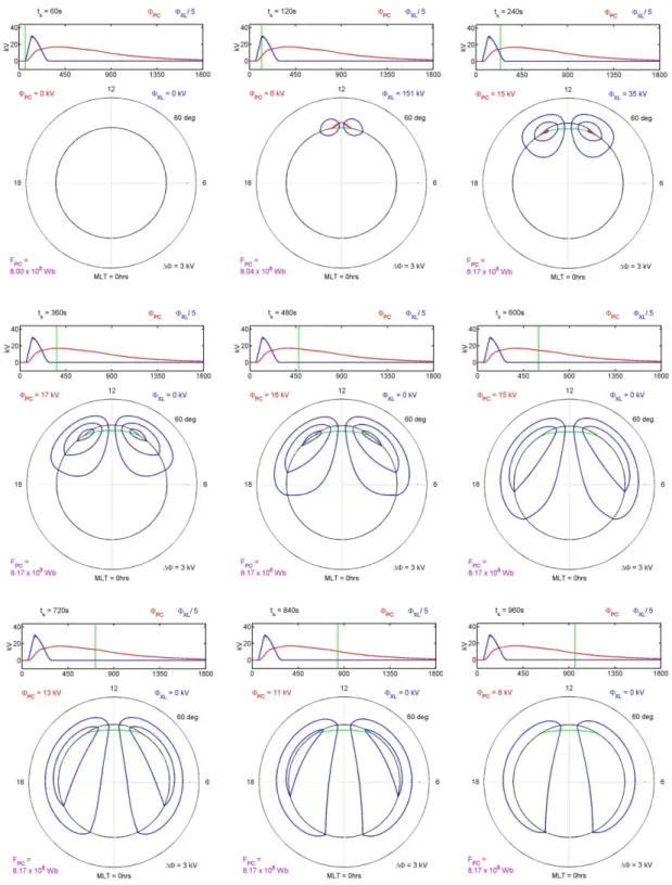
2.2 Modelled convection and ion temperature variations The example results presented in Paper 1 are for a merging gap centred on 13 MLT and the reconnection rate variation specified with two pulses of reconnection. The repeat period was set at 8 min, that characteristic of putative signatures of reconnection bursts at the magnetopause called flux transfer events (Rijnbeek et al., 1984; Lockwood and Wild, 1993).
This paper presents a simpler reconnection specification. The centre of the merging gap is located at noon MLT and a single reconnection pulse is applied to the X-line. The pulse lasts 1 min at each MLT it propagates over and adds a to-tal open flux of 1.85×10⁷Wb (2.3% of the pre-existing to-tal). All the other inputs are as in Paper 1. Figure 2 gives the modelled boundary locations and convection patterns for the reconnection specification used in this study. Each frame shows the pattern of flow streamlines, above which is the variation of the input reconnection voltage, integrated along the X-line, 8XLand the output transpolar voltage, 8P C. The vertical green bar in each panel shows the simulation time of the convection pattern below.
The model has also been extended to calculate ionospheric ion temperature, and the convection enhancement is studied here using the model response in ion temperature, Ti. This is because ion temperature is a scalar quantity and thus is not dependant on viewing angle, which makes it very use-ful for detecting motions and changes of fast flow regions. Indeed, the expansion of the convection pattern was first
S. K. Morley and M. Lockwood: Measuring expansions in the ionospheric flow response 2503
IN
PU
TS
ReconnectionVariation Initial Conditions Constants) , , ( ) (MLT, OCB E OCB s f t τ Λ Λ = cn V ) (MLT,ts ε V′(MLT,ts) ) , (MLTt ε ) , ( ) (MLT, cn b V V V ts =f ′ s s s t t t = +∆ s s OCB s s OCB t t MLT t t ∆ + Λ = ∆ + Λ b V ) , ( ) (MLT, OCB s OCB s s OCB F t F t t F ∆ + = ∆ + ) ( ) ( MLT, MLT,
OUTPUTS
Secondary Products Convection Pattern ) , , (ΛMLTts Φ ) , ( s OCBMLTt Φ ) ( for ) ( of n Computatio MLT, E s s OCB s s t t F t t ∆ + ∆ + Λ 0 ) 0 ( ) 0 ( = = Λ = Λ s s E s OCB t t t s r OCB t d dϕ/ τ ) (s PCt ΦI.1 I.2 I.3
A B C D E F G H O.1 O.2 O.3 O.4
Fig. 1. Flowchart describing the operation of the model presented in Paper 1. Inputs to the model are shown in boxes I.1, I.2 and I.3. Model processes are shown in the boxes labelled A-H. Outputs are shown in boxes 0.1–0.4. (see text for further details).
detected by Lockwood et al. (1986) using incoherent scat-ter radar measurements of ion temperature. A similar scalar that has been used for this purpose is the magnitude of the horizontal magnetic deflection seen on the ground, which is dominated by the effect of the Hall currents associated with convection. However, because magnetometers are sensitive to currents over an extended region and are influenced by horizontal structures in conductivities, these data are not as straightforward to interpret in the real ionosphere as the ion temperature data. We use a first-order approximation to the ion temperature:
Ti =Tn+
mn 3kB
(Vi−Vn)2 (1)
where Tn is the neutral temperature, kB is the Boltzmann constant, mnis the neutral mass, Vi and Vn are the ion and
neutral drift velocities. The terms on the right-hand side of Eq. 1 represent heat exchange with the neutral gas and direct ion–neutral frictional heating. The largest term neglected in Eq. 1 is heat exchange with the electron gas, and this may lead to a consistent underestimation of Ti by some tens of degrees (St. Maurice and Hanson, 1982). For simplicity it is assumed that Vn is zero in this model. This is satisfactory as we are interested in the change in ion temperature and the neutral wind is not believed to respond on timescales as short as the response of the ionospheric flows. Equation 1 also assumes that one neutral species dominates the atmospheric composition in the upper F-region ionosphere (St. Maurice and Hanson, 1982). The neutral particle mass, mn, is set to 16 a.m.u. (atomic oxygen).
For each timestep of the model the ion temperature at a se-ries of simulated stations at a constant latitude is calculated.
Fig. 2. Multiple output convection patterns from the model. Each frame has two panels. The top panel shows the variation with simulation time, ts, of the input reconnection voltage (in blue), 8XLdivided by five to fit the same scale as the resulting transpolar voltage (in red),
8P C. The simulation time of the output frame is marked by the vertical green line. The lower panel shows the convection pattern (using
3 kV equipotentials) plotted in an MLT-invariant latitude coordinate system. The outer circle represents the equatorward boundary of the modelled region and the inner circle represents the OCB. Non-reconnecting segments of the OCB are shown in black, while active x-line footpoints are marked in red. The green line delineates the region of newly-opened flux. The convection plots are shown with a two minute spacing, except for frame (a) (top row, left column) which is for ts=60 s.
S. K. Morley and M. Lockwood: Measuring expansions in the ionospheric flow response 2505 As there is a symmetry about the noon-midnight meridian,
we here employ a latitudinal ring of 72 simulated stations in the dawn hemisphere (at 67◦; i.e. outside the polar cap), with a 2.5◦(equivalent to 10 min of MLT) spacing. Note that the polar cap is centred on a latitude of 90◦ in the frame used and not offset towards the nightside as in a conventional ge-ographic or geomagnetic frame. Therefore, using a station latitude of 67◦ in this frame ensures that the (equilibrium) OCB is equidistant from the station at all MLTs. This al-lows us to isolate the azimuthal expansion of the convection pattern (i.e. it is not mixed with any latitudinal expansion).
3 Methods of deriving expansion velocities
From the point of view of detecting propagation speeds, an ideal situation would be to have a time-series observation from one measuring station which is identical to the obser-vation at another station, subject to a time lag. However, in real stuations the variation waveform and amplitude is not the same at different locations. Some of the problems as-sociated with observing propagation speed are illustrated in Fig. 3. The top panel shows a modelled ion temperature se-ries, taken from a simulated station at 10:05 MLT (just out-side the extent of the merging gap). The black dash–dot line marks the time when the ion temperature exceeds a selected fixed threshold (in this example we use 1010 K, shown by the blue dashed lines). The middle panel shows the ideal case, where the same data sequence is reproduced at a dif-ferent location after a time lag. In this case the time lag (to the green dash–dot line) would be independent of thresh-old and cross-correlating the data series would give a per-fect match and show the same time lag as threshold analysis. The lower panel shows the model data for a simulated station at 07:49 MLT. The red dashed line shows when the obser-vations from this simulated station exceed the same 1010 K threshold. As can be seen here, the waveform of the response varies with location and so the time lag derived will depend on the threshold used. This point was also raised by Ridley et al. (1999) and the same form of response seen in the model time-series in Fig. 3 can also be seen in the magnetometer data in their Fig. 4. Cross-correlating these data series will no longer find a perfect agreement and the differences in the growth and decay of the compared data series will introduce an extra lag (which can be positive or negative).
The expansion of the convection response to changed re-connection can be derived in several ways. This paper will examine methods we characterize as: 1) cross-correlation of the variation seen at a station with that from a fixed reference station; 2) cross-correlation using a floating reference station (e.g. comparing data from a station with that from it’s nearest longitudinal neighbour); 3) comparing times when the scalar exceeds a fixed level threshold; and 4) comparing times when the scalar exceeds a threshold that is a fixed percentage of the peak response at that station. Analysis of the movement of the peak is a limiting case of the threshold analysis (4) using a 100% threshold relative to peak.
1000 1020 1040 1000 1020 1040 Ion Temperature [K] 0 200 400 600 800 1000 1200 1400 1000 1020 1040 Simulation Time [s]
Fig. 3. A three-panel plot showing model ion-temperature time
series. The top panel shows data from a simulated station at
10:05 MLT; the middle panel is the same data lagged by 140 s; the lower panel is data from a simulated station at 07:49 MLT. The blue dashed lines mark a 1010 K threshold and the vertical lines mark the times that the data series first exceeds the threshold.
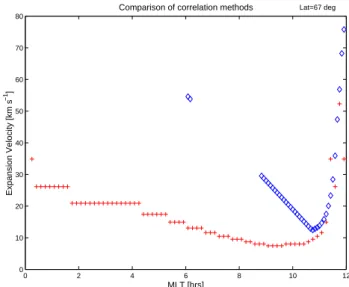
0 2 4 6 8 10 12 0 10 20 30 40 50 60 70 80 MLT [hrs] Expansion Velocity [km s −1 ]
Comparison of correlation methods Lat=67 deg
Fig. 4. A comparison of the velocities of the expansion of the model response to reconnection, derived by cross-correlation techniques (methods 1 and 2, respectively). The diamonds show the velocities derived by correlation with a fixed reference station (at 12 MLT), the crosses show the velocities derived using correlation with the adjacent (sunwards) station.
All of these methods determine the mean phase velocity,
VE, of the convection enhancement along the direction con-necting the pair of observation stations considered. The mean phase velocity, VE, is obtained from the best estimate of the propagation delay, 1tp. This yields, for stations separated by a distance 1l, VE=1l/1tp.
Specifically, for method (1) the data from each station, Si (where i=2, 3,. . . , n), is cross-correlated with the data from a fixed reference station, S1. 1tpis the lag that gives the peak
correlation. Method (2) is similar to method (1), except that the data from each station is cross-correlated with its nearest neighbour, Si−1. In method (3) 1tpis the delay between Ti rising above a fixed threshold at a pair of stations, whereas the threshold employed in method (4) is different for each station because it is a fixed fraction of the peak Ti seen at the station in question.
The cross-correlation analysis follows the same method regardless of our choice of reference station. To derive the expansion velocity of the response to reconnection we eval-uate the lag between datasets, x and y. We first find the cor-relation coefficient at the jt hlag, rj, between x and y for a range of lags: rj= "nj X i=1 xiyi+j− nj X i=1 xi nj X i=1 yi+j # nj X i=1 xi2− nj X i=1 xi !2 nj X i=1 yi+j2 − nj X i=1 yi+j !2 1/2 (2)
where nj is the number of pairs of common datapoints at lag j . The best correlated lag is then used to derive the mean expansion velocity between the simulated stations X and Y . If the temporal separation of datapoints is δt , the lag
1t=j δt. The lag giving peak rj is 1tp and the expansion velocity VE=1l/1tp.
As discussed above, two threshold techniques are used, ab-solute threshold levels and threshold relative to peak (meth-ods 3 and 4). Absolute thresholds are chosen by inspection of the data: we here use a range of thresholds for ion temper-ature between 1.001Tn and 1.02Tn, where Tn is the neutral exospheric temperature that is set at 1000 K. To determine the threshold relative to the peak temperature for each tion we find the maximum temperature measured at the sta-tion, Tm, and subtract a background component, taken here to be Tn, the exospheric temperature. The threshold for this station is then given as a fraction f of this change, added to the background, Tn+f (Tm−Tn).
Once the threshold is determined (by whichever method), each time series is searched for the first datapoint at which the ion temperature exceeds the threshold level. The times of passing threshold between adjacent stations are then sub-tracted to find the lag between stations. The model is run with time steps of 1 s: hence all lags less than or equal to 2 s are deemed undetectably small and not used. The derived lags are then used to deduce the mean expansion velocity.
Any derived expansion speeds should be compared with the expansion speeds that are inputs to the model. There are two such expansions, as discussed in Sect. 2.1. The first is inherent in the characterization of the reconnection rate vari-ation in space and time: changes in the reconnection rate propagate along the merging gap away from noon at 1 hour of MLT per 1.5 min, an expansion speed of 7.6 km s−1at an invariant latitude of 67◦. The second expansion is the veloc-ity with which the equilibrium boundary perturbation prop-agates towards midnight. This is set at 1 h MLT min−1,
cor-responding to 11.4 km s−1at 67◦latitude. This is the limit to how fast the OCB can react to the applied reconnection and will limit the expansion of the flow response. Close to noon (i.e. across the maximum extent of the merging gap), expansion is not limited by either of these two expansions. Rather, as the reconnection voltage increases, flow stream-lines will expand along the merging gap (10–14 MLT) ac-cording to Laplace’s equation (incompressible flow). 3.1 Cross-correlation methods
These common methods of finding response timescales avoid the complications of choosing a threshold and of how that threshold level conditions our interpretation of data (e.g. Etemadi et al., 1988). In investigating the convection re-sponse of the Lockwood and Morley (2004) model to im-posed reconnection voltage variations we consider the over-all response, as well as the onset. Selection of a reference point for timing the delay is of some importance to a study of the ionospheric response time (Ruohoniemi et al., 2002). Se-lecting either the moment of presumed arrival of the new IMF at the magnetopause, or the moment of presumed arrival of information (of this change in IMF) in the high-latitude iono-sphere would give rise to a timing uncertainty. Both options rely on estimating the propagation lag between the upstream monitor and the magnetopause. They also require knowledge of the magnetopause location and the Alfv´en wave travel time to the ionosphere. Thus they will add an uncertainty to the delay to onset of the ionospheric response.
To examine the propagation of the onset of change, as a function of MLT, we are concerned with the timing delay between data-series from different locations; this uses the moment of the first measured response at a location within the high-latitude ionosphere as a reference point. It will not affect the reconfiguration timescale after the arrival of infor-mation about the turning in the IMF. The uncertainties in the propagation of the IMF and the communication of changes in the IMF to the high-latitude ionosphere are problems that have been addressed in other studies (e.g. Ruohoniemi and Baker, 1998). Here we restrict the study to comparing the rel-ative response times, based on lags between locations around the auroral oval.
When performing a cross-correlation study comparing rel-ative response times within the high-latitude ionosphere, we have two options for a reference point. These are methods 1 and 2, namely correlation with either a fixed reference or a floating reference point. We here cross-correlate the model temperature time series against the variation modelled at a fixed point (taken here to be noon).
Figure 4 compares the velocity of expansion of the mod-elled convection response to reconnection, as a function of MLT and for fixed latitude, as derived using cross-correlation with a fixed reference (method 1, blue diamonds) and a ing reference (method 2, red crosses). In this case, the float-ing reference is the adjacent station on the sunward side. The limitations of correlation with a fixed reference is immedi-ately apparent in the extent of derived expansion velocities,
S. K. Morley and M. Lockwood: Measuring expansions in the ionospheric flow response 2507 whereas the model is constructed with just two expansion
ve-locities. The velocity derived is an average velocity between the reference station and the comparison station, hence must be applied to the mid-point. As the separation from a fixed reference point increases, average speeds are more accurately measured. However, there is more variation about that mean between the stations and if that variation is not linear the ac-tual value at the midpoint will not be accurately measured.
One major disadvantage of using a fixed reference is that the modelled time series does not maintain a constant shape across different stations and the differences become more marked at larger separations. Thus this method very rapidly loses good correlation as station separation increases and the significance of the result becomes very low. This shape change can be minimized by correlating with an adjacent sta-tion, however this reduces the time lag and leads to a higher measurement error.
3.2 Threshold methods
Figure 5 shows plots of the convection response expansion velocities obtained using fixed threshold analysis. The major problem associated with this technique is that as we increase the threshold we become further removed from examining the propagation of the onset of change – measuring the actual onset would require us to be able to detect an infinitesimal change from the background. To examine the propagation of the onset of change the threshold selected must be as low as the noise level in the background allows. As the thresh-old is raised, the characteristic expansion observed is that of a higher level of response which will not necessarily propagate with the same velocity, or even over the same extent. For ex-ample, using magnetometer data, Murr and Hughes (2001) have demonstrated the expansion of the convection pattern but noted that the expansion velocity depended on which fea-ture of the response was studied. The effect on the derived velocities can be seen in Fig. 5 as the threshold is increased. Further, the ion temperature distribution is not uniform and any temperature enhancement at the reconnection footprint will decay as it propagates around the auroral oval. This ef-fect means that following a fixed threshold artificially slows the observed propagation of the convection response; that is, we will underestimate the rate of expansion. This effect be-comes more pronounced both as we move further from the reconnection footprint, and as higher thresholds are chosen. A further effect of following a fixed threshold as the ion tem-perature decays is that eventually the temtem-perature will drop below the threshold value and the expansion can no longer be monitored.
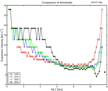
To eliminate this problem, we can take a threshold that will always be present at a given simulated station, i.e. we use a fixed percentage of the (background subtracted) maximum value as the threshold for that location. Figure 6 shows the response as determined by this relative threshold analysis.
The derived expansion velocities at relative thresholds closer to the peak value naturally reflect the bulk response, rather than the propagation of onset. This effect can be seen
0 2 4 6 8 10 12 0 5 10 15 20 25 30 35 40
Comparison of thresholds (Lat=67 deg)
MLT [hrs] Expansion velocity [km s −1 ] 1001 K 1005 K 1010 K 1015 K 1020 K
Fig. 5. A comparison of the velocities of the expansion of the model response to reconnection as determined using fixed threshold analy-sis (method 3). The threshold temperatures are absolute values, and are set at intervals above the input neutral temperature, 1000 K.
0 2 4 6 8 10 12 0 5 10 15 20 25 30 35 40 Comparison of thresholds MLT [hrs] Expansion Velocity [km s −1] 10% 37% 50% 80% Lat=67 deg
Fig. 6. A comparison of the velocities of the expansion of the re-sponse to reconnection as determined using relative threshold anal-ysis (method 4). The threshold temperatures are calculated as a percentage of the peak temperature change measured for each sim-ulated station.
to be more pronounced using an 80% (of peak) threshold level than using a cross-correlation (correlating the entire data-series). As the threshold level is reduced, as a fraction of the peak response, the derived velocities more closely re-semble the expected form of the initial response.
4 Discussion
The results shown in Figs. 4, 5 and 6 can be compared with the expansion speeds that are inputs to the model. The two
Modelled Ion Temperature, T i [K] 1000 1005 1010 1015 1020 1025 1030 1035 200 400 600 800 1000 1200 10 20 30 40 50 60 70 Simulation time, t s [seconds]
Simulated station number
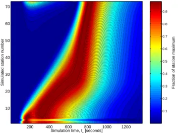
Fig. 7. A formedogram showing the ion temperature response with time, at various MLT (for a fixed latitude, here 67◦). The scenario modelled is for a single burst of reconnection, starting at ts=60 s
and having a duration of 1 min at all MLT from 12 MLT to 10 MLT (in bins of (360/256)◦). The expansion velocity of the X-line foot-print at 67◦latitude is 10◦min−1. The station numbered 1 is at 12 MLT and station number 72 is at 0 MLT.
Fraction of station maximum
0.1 0.2 0.3 0.4 0.5 0.6 0.7 0.8 0.9 200 400 600 800 1000 1200 10 20 30 40 50 60 70
Simulation time, ts [seconds]
Simulated station number
Fig. 8. A formedogram of the model Ti response (see Fig. 7),
nor-malized to the local maximum for each simulated station.
expansions, discussed previously, are reiterated here. The first is inherent in the characterization of the reconnection rate variation in space and time: changes in the reconnection rate propagate along the merging gap away from noon at 1 hour of MLT per 1.5 min, an expansion speed of 7.6 km s−1 at an invariant latitude of 67◦. The second expansion is the velocity with which the equilibrium boundary perturbation propagates towards midnight. This is set at 1 h MLT min−1, corresponding to 11.4 km s−1 at 67◦ latitude. Across the maximum extent of the merging gap (10–14 MLT), expan-sion is not limited by either of the two expanexpan-sions that are explicitly input into the model. Rather, as the reconnection voltage increases, flow streamlines expand along the merging
gap according to Laplace’s equation (incompressible flow). Outside the merging gap we expect the speed of 11.4 km s−1
to dominate.
Because we are examining the onset of the ionospheric convection response to reconnection we need to minimize the effects of the peak flow on our determination of the ex-pansion. This means that cross-correlation is not a suitable method for studying the onset of convection – it is ideal for examining the bulk response. Figure 5 shows that the in-put expansion velocity of 11.4 km−1is well recovered over a large range of MLT outside the merging gap (2–10 MLT on the dawn flank presented), but the accuracy and the range of MLT that it can be used over decreases as the threshold is increased. Therefore, using a fixed threshold will follow the onset (given a sufficiently low threshold above the back-ground), but raising the threshold increases the errors in the expansion speed recovered and too low a threshold intro-duces problems with noise or spatial structure in the mea-sured background level. This effect will be most marked if the reconnection pulse is small and the flow is weak; conversely, a large pulse and a stronger response will give smaller errors. Taking the threshold as a percentage of the maximum change in each data series will be conditioned to a degree by the the bulk flow, as can be seen by following the 100% threshold, equivalent to the movement of the peak re-sponse. However, this method does have the advantage over fixed threshold that the threshold always exists for a given station at which there is a detectable response. Figure 6 shows that taking a threshold of 10% of the peak change, applicable to real data where better than 10% noise is at-tainable, gives better than 20% accuracy for much of the re-gion where the velocity of the OCB perturbation dominates the flow expansion (6–10 MLT). However, increasingly on the nightside this method overestimates the expansion speed. This is because of the non-linear nature of the ion tempera-ture rise (see Eqs. 1), an effect that would not be present for other scalars (such as the magnetometer perturbation).
To help us interpret these findings, Fig. 7 shows the ion temperature profile as a function of time and station num-ber (which varies linearly with MLT from noon for station 1 to midnight for station 72). This formedogram (from the greek “formedon” – meaning “in layers crosswise”) has a very high information content and provides a powerful means of presenting the data. Analysis by fixed threshold follows an isotherm, i.e. the expansion velocity at any given ion temper-ature threshold level can be seen as the slope of that contour on the formedogram. The movement of the peak response is easily seen on a formedogram, as is the change of shape of the response profile with MLT (i.e. with station number). By subtracting the background (here the neutral exospheric temperature) and normalizing the measured ion temperature change relative to the maximum change for each simulated station, the formedogram shows contours of relative change. Figure 8 shows the model Ti response seen in Fig. 7 but here the response measured at each simulated station is normal-ized to the maximum at that station. From these plots it can be seen that the relative threshold technique performs well
S. K. Morley and M. Lockwood: Measuring expansions in the ionospheric flow response 2509 in recovering the expected expansion in the modelled
iono-spheric ion temperature, at least up to station 35 (i.e. dayside MLTs). Further onto the nightside the expansion is overes-timated, particularly for the higher relative thresholds. As we are using a relative threshold we do not see the artificial slowing of the expansion due to the higher temperatures not propagating all the way around the polar cap.
The temperature anomaly seen in station 3 of Fig. 7 arises due to the proximity of the active reconnection X-line foot-print. The equatorward edge of the active reconnection re-gion has strongly enhanced ion temperatures and as the OCB erodes equatorward and propagates away from noon the en-hancement is seen at station 3. It is only seen at this sta-tion as the bulge relaxes equatorward as the X-line footprint propagates towards midnight. Examination of the effect of latitude on the anomalous temperature enhancement shows that the magnitude of the anomaly is diminished at lower latitudes and is not observed inside the polar cap. This is also observed in Fig. 8 across all simulation times as the en-hancement gives a much higher peak to which the data is nor-malized, suppressing the lower temperatures. The apparently quasi-instantaneous response seen at midnight in Fig. 8 arises from numerical noise in the model being amplified during the normalization and is of order 0.1 K.
5 Conclusions
The Lockwood and Morley (2004) numerical model has been used to simulate a convection response to a single pulse of re-connection. Using a first-order approximation, the model has been extended to simulate the scalar ion heating response. From the input variation in reconnection rate the model pro-duces a Cowley–Lockwood (1992; 1997) type expanding twin-vortex convection pattern and hence the variation of ion temperature associated with this convective flow. The onset of the convection response will propagate around the high-latitude ionosphere with a characteristic angular veloc-ity. Cross-correlation, fixed threshold analysis and threshold relative to peak are used to determine the expansion velocity. Each of these methods fails to recover fully the expansion of the onset of the convection response – this is the veloc-ity with which the equilibrium boundary perturbation due to the newly opened flux is responding. The closest estimate to the model input speed of 11.4 km s−1is obtained for a fixed
threshold that is very low. However, for real (as opposed to simulation output) data, noise fluctuations will not allow such low enhancement thresholds to be used. The effect of measuring technique on the interpretation of a model expan-sion is pronounced. Cross-correlation (across the entire event interval) follows the peak response, i.e. the response of the bulk flow, rather than the onset of flow. This effect can be re-duced by selecting a different correlation window (this study used the entire data series), but the selection of the corre-lation window will affect the result and it is by no means certain what should be chosen.
The merits of using either time-series data or convection maps have been discussed in depth by Freeman (2003). Free-man contrasted model results from implementations of the REA model and a variant of the CL model. In the variant Cowley–Lockwood model employed by Freeman (2003), as the entire polar cap is allowed to respond simultaneously, the onset will be globally simultaneous. They concluded that, for the “standing wave” (REA) solution and “travelling wave”’ (variant CL) solution, the distinction between the models is least evident in global convection maps. Ruohoniemi et al. (2002) have also raised questions about the accuracy of the “residual potential” maps used by Ridley et al. (1998). These considerations show that time-series data is the most useful for distinguishing between the competing models, provided there is reasonable data coverage. Further, the results of this study indicate that any expansion of the convection pattern will be best observed in time-series data using a threshold relative to peak.
These different measuring techniques have potential for discriminating between models of ionospheric convection re-sponse. If the convection pattern shape is fixed, as in the REA model, then a cross-correlation study would show a si-multaneous response. Further, as they state that the pattern is fixed and the strength increases linearly (Ridley et al., 1998) we would not expect to see any expansion using a thresh-old relative to peak. In the CL model an expansion will be observed using all methods (even if the derived expansion speeds are not generally accurate). Since both the convec-tion pattern and strength vary with time, cross-correlaconvec-tion will still recover the bulk flow. Given sufficiently clean data the simultaneity of onset may be revealed using a low thresh-old relative to peak. In any of these cases an expansion will be observed using a fixed threshold, though this may be mis-leading as Ridley et al. (1999) pointed out. Following a fixed threshold level will show an expansion even for a fixed pat-tern of convection, provided it is increasing in strength.
Acknowledgements. The authors thank B. Lanchester for helpful suggestions and support. This work was supported by the UK Par-ticle Physics and Astronomy Research Council.
Topical Editor M. Pinnock thanks S. Milan and another referee for their help in evaluating this paper.
References
Cowley, S. W. H. and Lockwood, M.: Excitation and decay of solar-wind driven flows in the magnetosphere-ionosphere sys-tem, Ann. Geophys., 10, 103–115, 1992.
Cowley, S. W. H. and Lockwood, M.: Incoherent scatter radar ob-servations related to magnetospheric dynamics, Adv. Space Res., 20 (4/5), 873–882, 1997.
Etemadi, A., Cowley, S. W. H., Lockwood, M., Bromage, B. J. I., Willis, D. M., and L¨uhr, H.: The dependence of high-latitude flows on the North-South component of the IMF: A high time resolution correlation analysis using EISCAT ”Polar” and AMPTE UKS and IRM data, Planet. Space Sci., 36, 471–498, 1988.
Freeman, M. P.: A unified model of the response of ionospheric convection to changes in the interplanetary magnetic field, J. Geophys. Res., 108(A1), 1024, doi:10.1029/2002JA009 385, 2003.
Freeman, M. P., Ruohoniemi, J. M., and Greenwald, R. A.: The de-termination of time-stationary two-dimensional convection pat-terns with single-station radar, J. Geophys. Res., 96, 15 735– 15 749, 1991.
Khan, H. and Cowley, S. W. H.: Observations of the response time of high-latitude ionospheric convection to variations in the in-terplanetary magnetic field using EISCAT and IMP-8 data, Ann. Geophys., 17, 1306–1335, 1999,
SRef-ID: 1432-0576/ag/1999-17-1306.
Lockwood, M. and Cowley, S. W. H.: Comment on “A statistical study of the ionospheric convection response to changing inter-planetary magnetic field conditions using the assimilative map-ping of ionospheric electrodynamics technique” by A. J. Ridley et al., J. Geophys. Res., 104, 4387–4391, 1999.
Lockwood, M. and Morley, S. K.: A numerical model of the iono-spheric signatures of time-varying magnetic reconnection: I. Ionospheric convection, Ann. Geophys., 22, 73–91, 2004, SRef-ID: 1432-0576/ag/2004-22-73.
Lockwood, M. and Wild, M. N.: On the quasi-periodic nature of magnetopause flux transfer events, J. Geophys. Res., 98, 5935– 5940, 1993.
Lockwood, M., van Eyken, A. P., Bromage, B. J. I., Willis, D. M., and Cowley, S. W. H.: Eastward propagation of a plasma con-vection enhancement following a southward turning of the inter-planetary magnetic field, Geophys. Res. Lett., 13, 72–75, 1986. Lu, G., Cowley, S. W. H., Milan, S. E., Sibeck, D. G., Greenwald,
R. A., and Moretto, T.: Solar wind effects on ionospheric convec-tion: a review, J. Atmos. Solar-Terr. Phys., 64, 145–157, 2002. Murr, D. L. and Hughes, W. J.: Reconfiguration timescales of
iono-spheric convection, Geophys. Res. Lett., 28, 2145–2148, 2001.
Nishitani, N., Ogawa, T., Sato, N., Yamagishi, H., Pinnock, M., Villain, J. P., Sofko, G., and Troshichev, O.: A study of the dusk convection cells response to an IMF southward turning, J. Geo-phys. Res., 107, 1036, doi: 10.1029/2001JA900 095, 2002. Ridley, A. J., Lu, G., Clauer, C. R., and Papitashvilli, V. O.: A
sta-tistical study of the ionospheric convection response to changing interplanetary magnetic field conditions using the assimilative mapping of ionospheric electrodynamics technique, J. Geophys. Res., 103, 4023–4039, 1998.
Ridley, A. J., Lu, G., Clauer, C. R., and Papitashvili, V. O.: Reply, J. Geophys. Res., 104, 4393–4396, 1999.
Rijnbeek, R. P., Cowley, S. W. H., Southwood, D. J., and Russell, C. T.: A survey of dayside flux transfer events observed by ISEE 1 and 2 magnetometers, J. Geophys. Res., 89, 786–800, 1984. Ruohoniemi, J. M. and Baker, K. B.: Large-scale imaging of
high-latitude convection with Super Dual Auroral Radar Network HF radar observations, J. Geophys. Res., 103, 20 797–20 811, 1998. Ruohoniemi, J. M. and Greenwald, R. A.: The response of high-latitude convection to a sudden southward IMF turning, Geo-phys. Res. Lett., 25, 2913–2916, 1998.
Ruohoniemi, J. M., Shepherd, S. G., and Greenwald, R. A.: The response of the high-latitude ionosphere to IMF variations, J. At-mos. Sol.–Terr. Phys., 64, 159–171, 2002.
Saunders, M. A., Freeman, M. P., Southwood, D. J., Cowley, S. W. H., Lockwood, M., Samson, J. C., Farrugia, C. J., and Hughes, T. H.: Eastward propagation of a plasma convection en-hancement following a southward turning of the interplanetary magnetic field, J. Geophys. Res., 97, 19 373–19 380, 1992. St. Maurice, J. P. and Hanson, W. B.: Ion frictional heating at high
latitudes and its possible use for an in situ determination of neu-tral thermospheric winds and temperatures, J. Geophys. Res., 87, 7580–7602, 1982.