HAL Id: hal-00590892
https://hal.archives-ouvertes.fr/hal-00590892
Submitted on 5 May 2011
HAL is a multi-disciplinary open access
archive for the deposit and dissemination of
sci-entific research documents, whether they are
pub-lished or not. The documents may come from
teaching and research institutions in France or
abroad, or from public or private research centers.
L’archive ouverte pluridisciplinaire HAL, est
destinée au dépôt et à la diffusion de documents
scientifiques de niveau recherche, publiés ou non,
émanant des établissements d’enseignement et de
recherche français ou étrangers, des laboratoires
publics ou privés.
A Methodological Approach To Quantify The Effect Of
Flow Variability On Aquatic Population Dynamics
P. Breil, M. Lafont
To cite this version:
P. Breil, M. Lafont. A Methodological Approach To Quantify The Effect Of Flow Variability On
Aquatic Population Dynamics. Balwois 2008, May 2008, Orhid, France. 7 p. �hal-00590892�
A Methodological Approach To Quantify The Effect Of Flow
Variability On Aquatic Population Dynamics
Pascal Breil and Michel Lafont
Cemagref, Research Unit in Hydrology and Hydraulics, Lyon, France (email : [email protected])
ABSTRACT
The scarcity of biotic data versus the continuity of flow data is a first problem to be solve when trying to built a model of response to flow and related anthropogenic manipulations. Biotic - abiotic model building, for impact assessment or management purposes, requires mathematical links between biotic indices values and corresponding habitat conditions. Giving the fact that living species can integrate past habitat conditions in their behavior, correlations with instant habitat flow data from a biotic sampling moment are not adapted. This limit can be overcame developing a computer routine to calculate a series of antecedent Hydrological Indices (HIs) into incremented periods backwards in time from biotic sampling dates. Correlation analysis is used to select significantly related HIs to biotic indices resulting from sporadic surveys at a same location. This method allows to quantify the time of response of the biota and duration of effect of given HIs on this water course biota. We use for the
purpose time series for discharge, and when available, water temperature, flow velocity, water depth and repeated surveys for invertebrates and macrophytes.
Key words: flow variability, hydrological indices, biotic indices, correlation analysis
Introduction
The continental aquatic biota resource is mainly used for human consumption or like an indicator of the impairment resulting from the anthropogenic activity effect (see European Union Water Framework Directive). It is less used as a potential tool to help the aquatic system to stand in a “healthy” condition. This last application is by now a challenge whose key words are resilience and absorbing capacities. The way that flow variability influences the biotic dynamics in water courses remains a question because no simple relationships has been set up at the moment. On one hand, the present trend is to calculate a series of hydrological indices (Olden & Poff, 2003) to describe specific aspects of the flow regimes, to group water courses into categories and generate hypothesis on their expected effect on the water course biota. On the other hand, the calculation of optimal flow conditions for target aquatic species, mainly fishes, is based on the hydraulic modelling. In this approach habitat preference curves are built from expertise considering flow velocity, water depth and substrates grain size characteristics. The limit of the method comes from the averaging character of these curves that cannot include individual onsite environmental constraints like competition, predation or flow variability. Flow variation in time can be a main driver as it can modify rapidly and temporary local hydraulic conditions but also water temperature, turbidity, nutrients and pollutant flux, solid transport, all these factors controlling the aquatic biota energy loss and gain. An Attempt to combine both hydrological and hydraulic based methods (Sanchez et al. 2007) reveals that a high temporal fragmentation of suitable habitat conditions for an endangered species in Spain can explain its present population decline and at least extinction. There is a clear need to better link biota behavior both to its local hydraulic features but also to their temporal variations.
The dynamic modelling of a water course biota population is difficult to build because biotic data are often scarce over time and space. However one interesting point is that biota integrates past habitat conditions. The question is what are the driving conditions and from how long in the past are they influencing the present state.
Material and method
Interstitial macro-invertebrates
We consider in that case a small watercourse exposed to combined sewer overflows. The Chaudanne stream is located in the periurban area of Lyon (France). Crops and grasslands predominate in this watershed when a small urban area is rapidly developing in its downstream part. The watershed area
is 2.7 km2 at the first combined sewer overflow device where data collection was performed. There is a continuous record of flow data including natural stream flow and combined sewer overflows coming from a sewage network to the stream.
The biological assessment is based on oligochaete assemblages collected in a coarse porous sediment at two depth in the water course substrates . The first is the benthic layer which corresponds to the five first centimeters of sediments. The second is the hyporheic layer sampled thirty centimeters deep in the sediments. Two sites were sampled four times a year on a six years duration. Sampling sites were located 50 and 200 metres downstream a same Combined Sewer Overflows (CSO) device. Benthic sampling are referred later as S3 and S4 and hyporheic as H3 and H4. The upstream site (S3/H3) is a fast running water portion of the stream when the downstream site (S4/H4) is in a more lentic portion reflecting a change in the mean stream bottom gradient. These local geomorphic features can modify the effect of a same flow variability on their respective biota. The oligochaete species assemblages can be grouped into 4 biotic indices called here functional traits (FTrs). The FTr1 “permeability” is obtained by measuring the proportion (%) of oligochaete species which are indicators of active water exchanges between surface and groundwater (Lafont & Vivier 2006). The FTr2 is defined by the percentage of pollution-intolerant oligochaete species and is associated with good chemical quality of waters (Lafont et al. 2006). The FTr3 is defined by the percentage of water pollution-tolerant species. It is associated with poor chemical quality and particularly with high nitrate and ammonium salt contents. The FTr4 (“sludge effect”) is defined by the percentages of species living in fine sediment and sewage bacterial-bed. It indicates the presence of polluted sludge spread within sediment interstices, with very high ammonium salt contents, low nitrate concentrations and the significant presence of heavy metals (copper, zinc and lead). The gradient of FTrs has been validated through a range of water courses size across France (Vivier, 2006).
A total of thirteen Hydrological Indices (HIs) were computed from natural flow and CSOs time series. They described CSOs features like magnitude, amount, number, and duration, periods without CSOs and the natural mean flow. HIs were calculated backwards in time incrementing a time step of 10 days till 120 days before each biotic sampling date. It resulted into 12 Preceding Period Duration (PPDs) from 10 to 120 days. The objective was to identify what hydrological indices calculated from short to long term past flow conditions would explain the biotic indices. The long tem duration of 120 days was stated knowing the life span cycle of oligochaetes was established to be 60 to 90 days.
The time of response of the biota to HIs was calculated considering three situations and knowing the R correlation value was calculated each time the PPD was incremented of 10 days backwards in time from the date of sampling. First was when a HI resulted from extreme (maximum or a minimum) values observed in the past hydrological conditions. In this case we had to consider the fact these values could persist in the set of points when the PPD was increased. The smallest PPD was then retained as the time of response. Second was the case when HI was a the mean value of past natural flow conditions. In this case the good correlation along PPDs was the consequence of the flow stability. Then the time of response was considered to be the largest correlated PPD. Third was the case of the HI corresponding to the duration without CSOs before the higher CSO observed in the PPD. Longer was the duration better was the ecological quality. We then retain the medium PPD as the time of response..
A spearman rank correlation coefficient R was calculated for each PPD. This method was retained after testing for the non parametric distribution of the biotic indices. Correlations were computed using each functional trait (FTs) as the dependant variable and each hydrological indices (HIs) as the independent variable. It resulted in a table of 12 PPDs by 4 FTrs for each of the 4 sampling location S3, S4 , H3 and H4. Such a table was computed for each of the 13 hydrological indices (HIs). Only R rank correlation values over 0.5 with a significance level of 2% were retained for interpretation. The maximum of correlation (when observed) had to belong to a continuation of significant correlations to avoid any fortuitous (isolated) value along consecutive PPDs. We retained a minimum of 3 consecutive values as a threshold. It resulted in a synthetic table we discuss in the result part of this paper.
Running water macrophytes
A reach of 250 m long and 100 m wide, situated immediately upstream from a gauging station, was selected on the river Dordogne (France). From this point, the catchment drains about 14 000 km2. An extensive cereal crop activity in this region provides a lot of nutrients to the river. So nutrient supply is
not a limiting factor for the aquatic vegetation growth. Vegetation species and abundance, as well as the water levels and velocities along five regularly spaced cross sections were surveyed from 2001 to 2006 several times a year. For the vegetation survey, the pin-point method was used. Points were sampled every 2.5 m using a rake from a boat. For each sample, the species and its relative abundance from 1 (very scarce) to 5 (very abundant) were noted. The biotic indices was calculated as the percent cover which represents the frequency of colonized points weighted by the abundance. Aquatic macrophytes include different taxonomic groups with different morphologies and physiologies like bryophytes, pteridophytes and the most abundant in the samplings were phanerogams and algae. Then our study has focussed on these two last species.
Mean reach scale values for water temperature, flow velocity, water depth, and combinations of these physical factors were calculated before each biotic sampling date. Time durations backward from these dates were 1, 2, 4, 8, 16, 32, 64, 128, 192, 256 and 365 days long. The yearly maximum PPD was retain considering the annual life span cycle of macrophytes. As the same than for micro-invertebrates, R correlation coefficients were calculated.
Results
Interstitial macro-invertebrates
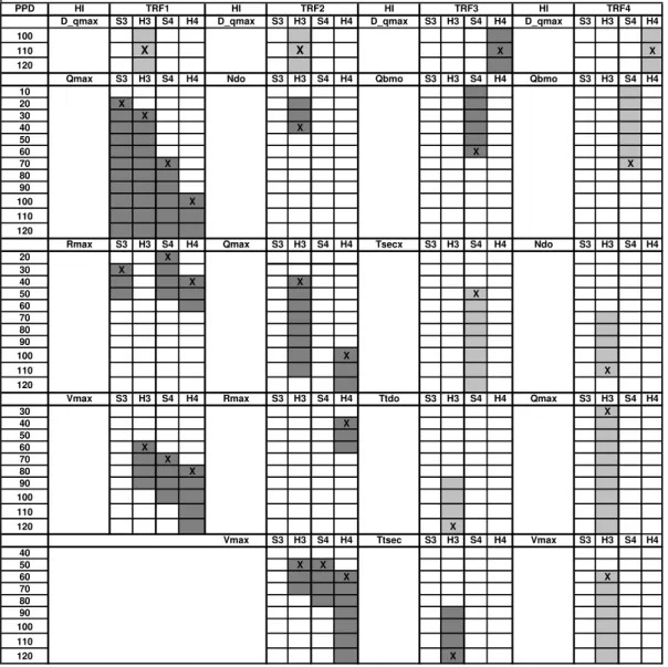
Ten HIs among the group of thirteen fit with the criteria of selection. Due to the number of HIs the results are presented in the form of a table (Table 1). Significant correlation values indicated in table 1 range from 0.5 to 0.89. They were calculated for each biotic indices (here four functional traits) at each sampling location (S3, S4, H3, H4) and are presented in columns. In the first column is the PPD in days unit. Then HIs of interest are indicated for the four locations. This pattern is repeated for each biotic indices (FTrs). A precise definition of HIs is given in the result interpretation.
Time of response of the biota is indicated by a cross. Dark and grey cells respectively indicate a positive (+) and a negative (-) correlation sign. The biotic indices, here called functional traits (FTrs), can be interpreted in terms of ecological quality improvement or degradation from FTr1 to FTr4. Thus positive correlations with FTr1 and FTr2 indicates the corresponding HIs are factors of ecological improvement (and reverse). On the contrary, positive correlations with FTr3 and FTr4 indicate the corresponding HIs are factor of ecological degradation. The physical and chemical meaning of the biotic indices can then be interpreted in the light of the temporal physical factors variations.
In the benthic layer S3 only the FTr1 correlates positively with Rmax and Qmax which correspond respectively to the maximum ratio of the peak CSO to the mean natural flow and to the maximum peak CSO. They both characterize maximum CSO event. The ecological quality is improving 20 to 30 days after the event. The associated physical process can be the renewal, mixing and aeration of the surface sandy substrate during the event. It is confirmed from field monitoring that for large CSOs the amount of pollution is greatly diluted by rain waters from urban runoff and after from the natural basin drainage. The pollution impact is reduced.
In the benthic layer S4 the good ecological quality improvement (with FTr1) is again explained by Qmax, Rmax and Vmax. The response time is short only for Rmax (20 days) when it reaches 70 days for Qmax and Vmax. FTr2 correlates also positively after 50 days, then before FTr1, with Vmax. It indicates the ecological quality is improving with time. We can argue for the same physical cleaning process than for FTr1 at S3. The poor water chemical quality indicator FTr3 increases with Qbmo, the mean natural flow, since 60 days before the sampling date. At the same time the “polluted sludge” indicator FTr4 regresses also with Qbmo since 70 days before the sampling date. This temporal gradient of ecological and water quality improvement (from FTr4 to FTr3) probably results from the good quality water renewal in S4 during persistent natural flow conditions. Such conditions are related to important rainfalls that can generate great CSOs as the correlation with Qmax, Rmax and Vmax tends to confirm. FTr3 can also regress with Tsecx, the maximum dry sequence observed 50 days before. It globally means that ecological quality at S4 can improve in the absence of CSOs and with the persistence of a natural flow.
The hyporheic layers H3 and H4 are all correlated with D_qmax. Correlation signs are negative for FTr1 and FTr2 at H3. It means that longer is the time of the dry sequence before a major CSO, larger
is the degradation of the ecological quality. It can be explained by the fact that pollution accumulates on urban surfaces and develops in sewer pipes during dry sequences. Then the amount of pollution delivered to the stream system can be great. Surprisingly, the ecological quality seems to be improved at H4 because larger is the dry sequence smaller is FTr4 and larger is FTr3. In fact, site S4/H4 is a natural deposit site and a long dry sequence seems to improve the ecological quality of this site. Thus H3 seems to be more sensitive to large pollution loads linked to large CSOs and H4 seems to be more sensitive to frequent CSOs with medium pollution load.
Table 1. Spearman coefficient sign (dark = positive; grey = negative) for the rank correlation of functional traits (FTrs) versus hydrological indices (His). Cross into boxes indicates the time of response of the biota.
PPD HI HI HI HI
D_qmax S3 H3 S4 H4 D_qmax S3 H3 S4 H4 D_qmax S3 H3 S4 H4 D_qmax S3 H3 S4 H4
100
110 X X X X
120
Qmax S3 H3 S4 H4 Ndo S3 H3 S4 H4 Qbmo S3 H3 S4 H4 Qbmo S3 H3 S4 H4
10 20 X 30 X 40 X 50 60 X 70 X X 80 90 100 X 110 120
Rmax S3 H3 S4 H4 Qmax S3 H3 S4 H4 Tsecx S3 H3 S4 H4 Ndo S3 H3 S4 H4
20 X 30 X 40 X X 50 X 60 70 80 90 100 X 110 X 120
Vmax S3 H3 S4 H4 Rmax S3 H3 S4 H4 Ttdo S3 H3 S4 H4 Qmax S3 H3 S4 H4
30 X 40 X 50 60 X 70 X 80 X 90 100 110 120 X
Vmax S3 H3 S4 H4 Ttsec S3 H3 S4 H4 Vmax S3 H3 S4 H4
40 50 X X 60 X X 70 80 90 100 110 120 X TRF1 TRF2 TRF3 TRF4
In the hyporheic layer H3 improvement of ecological quality is again linked to Qmax, Rmax and Vmax for FTr1 and Vmax, and Ndo for FTr2. The physical effect of large CSOs has already been discussed. The biota response time for Ftr1 and Tr2 with Vmax again illustrates the gradient of improvement which starts at 50 days for Ftr2 and at 60 days for FTr1. The improving effect of the number of CSOs (Ndo) on H3 can be explained by the associated flow variability. This variability induces variable water head gradients in banks and substrates of the water course not far from the CSO device like for site S3/H3. It would emphasize the exchange of water between the surface and hyporheic layers (Breil et
al. 2007). Then the just downstream CSO receiving waters would benefit from frequent inputs of
nutriments but also from an activation of the biotic metabolism in the water course substrates. For FTr3, Ttdo and Ttsec are both correlated for the same PPDs but with opposite signs. This is because these HIs are strictly complementary to the total duration of each PPD. It means the ecological quality
is improved as the total duration of CSOs increases. This is in accordance with the effect of Ndo on FTr2 as exposed before. The biota response time is however longer (110 days) than for FTr2 (40 days) which can illustrate the kinetic of cleaning processes in the FTrs. FTr4 is always negatively correlated to Ndo, Qmax and Vmax for this layer. Again the ecological quality is improved when CSOs number increases and large CSOs occur. This is in accordance with other correlated FTrs in this layer. In the hyporheic layer H4 the ecological quality is again improved by Qmax, Rmax and Vmax both for TFr1 and TFr2. It confirms H4 requires great CSOs event to be cleaned. Also biota response time is larger than for H3. A great CSO event is normally followed by a natural flood in the water course. The S4 surface layer is then cleaned or removed which can reconnect surface and hyporheic waters. This process can explain a longer time of response and improvement of the biota.
Running water macrophytes
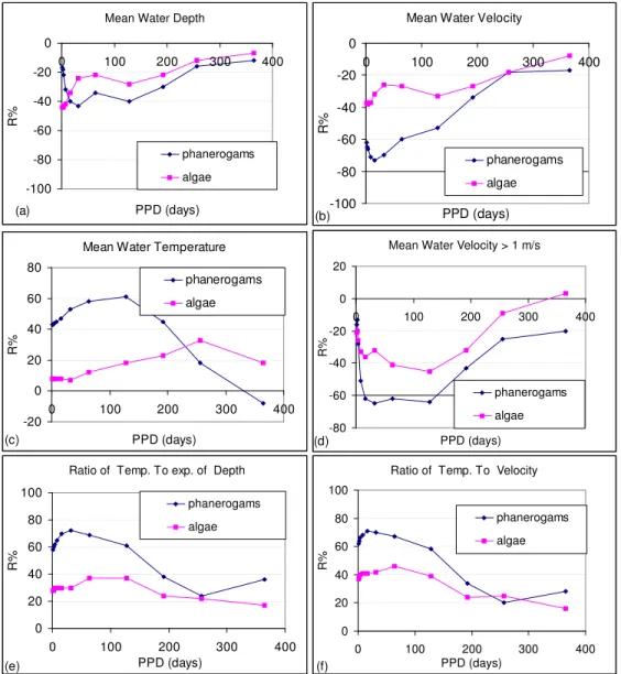
In this case-study no water quality perturbation is considered. We only know the nutrient load to the river from surrounding agricultural practices is important enough to not be a limiting factor for macrophytes development. Then only physical factors are considered. Correlation are presented into figure 1 (a) to (f).
Mean Water Velocity
-100 -80 -60 -40 -20 0 0 100 200 300 400 PPD (days) R % phanerogams algae Mean Water Depth
-100 -80 -60 -40 -20 0 0 100 200 300 400 PPD (days) R % phanerogams algae
Ratio of Temp. To exp. of Depth
0 20 40 60 80 100 0 100 200 300 400 PPD (days) R % phanerogams algae Mean Water Temperature
-20 0 20 40 60 80 0 100 200 300 400 PPD (days) R % phanerogams algae
Ratio of Temp. To Velocity
0 20 40 60 80 100 0 100 200 300 400 PPD (days) R % phanerogams algae Mean Water Velocity > 1 m/s
-80 -60 -40 -20 0 20 0 100 200 300 400 PPD (days) R % phanerogams algae (a) (d) (e) (b) (c) (f)
Figure 1 (a) to (f) : R2 correlation values evolution of hydrological indices (HIs) with biotic indices. R2 is plotted as a function of the Preceding Period Duration (PPD) on which HIs are calculated backward in time from biotic sampling dates.
Graphs give the evolution of the R value from recent past conditions to yearly integrated conditions. Absolute value of maximum correlation can be considered as the time of response of the biota to past hydrological conditions. From figure 1 (a, b, c) it seems that algae is few correlated with water temperature, water depth and water velocity. An explanation would be that algae are rapidly responding to physical changes and that frequency of sampling is not sufficient to catch these changes. It is also noticeable that water depth and velocity are negatively correlated with macrophytes. It gets sense considering that water depth and velocity are also correlated into water courses and that velocity can reduce the macrophytes development. Mean water temperature correlates positively with the biotic indices indicating that higher is the mean temperature greater is the % cover of macrophytes in the study reach of this river. Mean water temperature was tested to be quite independent from water depth and velocity. It does not give the same information.
Considering phanerogams, the mean water depth is the less correlated physical factor. The mean water velocity mainly correlates with conditions that occurred from 10 to 30 days before. Phanerogams are also sensitive to water temperature that occurred from 60 to 120 days before dates of sampling. If we consider mean water velocities over a threshold of 1 meter per second (fig. 1. (d)) we can observe that R increases from short to medium PPDs values of around 100 days. It can be interpreted as a scouring effect of water velocity both on algae and phanerogams. This is clearly a physical regulator of macrophytes in this reach.
The HI calculated as the ratio of the water temperature to the exponential of the water depth (fig 1. (e)) is sensitive both for algae and phanerogams for short to medium PPD values. The exponential value of the water depth is a surrogate measure of the turbidity. More pronounced it is, less the sunlight can penetrate the water column. The expected effect is to reduce the biotic indices. On reverse higher is the water temperature greater should be the biotic indices as a result of temperature effect on the aquatic plant metabolism. It is confirmed by the positive sign of the correlation. Replacing “turbidity” by the water velocity results in a sensitive improvement of the R values for algae. It indicates that algae are more sensitive to the water velocity than phanerogams.
DISCUSSION
The aim of this paper was to asses the contribution of past flow conditions on the biotic response in water courses. This issue was addressed developing a computer routine to calculate a series of antecedent hydrological indices (HIs) into incremented periods backwards in time from each sampling date. A large river and a small stream were considered. Only a part of the biotic indices can be explained by the hydrological factors meaning that also biotic factors should be considered like competition and predation. However from the presented methodological approach it is possible to get interesting information. A first one is the notion of a varying biotic memory length with flow (or associated flux) variability factors. A second one is the set of physical processes that can be associated to the observed correlations, in particular between surface and grounwaters (Boulton & Hancock 2006; Breil et al. 2007). A third one concerns flow management rules that can be used to preserve an ecological balance (Breil & Lafont 2007). These points are discussed here under from the presented results.
Macro-invertebrates : Mean response time of FTr1, FTr2, FTr3 and FTr4 are respectively of 57, 65, 92 and 81 days. It indicates the most reactive FTrs are FTr1 followed by FTr2 which depend mainly on flow transfer capacity . Then come FTr4 and FTr3 which take on average 30 days more to be reflected by the biota. An explanation would be that biotic metabolism are slower to reduce pollution than only physical based processes that are inherent to FTr1 and FTr2. The mean response time values of S3, H3, S4 and H4 layers are respectively of 25, 73, 56 and 88 days. It indicates the effect of HIs requires longer time to be reflected by the biota living in the deeper porous media (H3, H4). Several explanations arise: it can result from the lower flow velocity in the deeper layers or from the lower kinetics of the biotic metabolism in these layers or either from the predominance of physical mechanisms, like scouring, in the surficial layers. Also the time of response increases going downstream from S3/H3 to S4/H4 when comparing the same layers. This is quite understandable as the pollution can accumulate and be removed from place to place along time. We must also consider the bottom stream gradient is lower at S4/H4 than at S3/H3, which facilitates deposits of pollutants from the water column an transported substrates. As all the TFrs were present in each layer excepted for S3 our result can be interpreted as follow : the resilience capacity of the studied aquatic ecosystem is governed both by physical and biological factors. Two months on average are necessary to get an improvement of the ecological quality when there is only a slight to moderated pollution level. The management of flow dynamics (and water quality) would be sufficient to recover a good ecological
quality. Three months are required for more impacted situations. In that case, natural metabolism should be given more time to bio-assimilate the pollution load. It would be implemented using a storm water detention tank with adequate management rules.
Macrophytes : High velocities were observed to be responsible for the decreasing abundance of vegetation, due to the snapping or uprooting of the macrophytes during high water events (this is supported by Riis & Biggs 2003, Riis et al. 2004). Among the abiotic factors able to explain and control the aquatic vegetation dynamics, we found that no single variable could be retained. It seems that combinations of mean physical habitat conditions on long and medium terms control the macrophytes’ natural growth rate. Meanwhile, short duration events can increase or decrease it. The variability in time and space of the aquatic habitat conditions are expected to regulate the natural growth process of the aquatic vegetation.
Overall, the time of response can be interpreted as follow : the time with no correlation before the response would correspond to the resistance capacity of the biota to the changing habitat conditions. It can also include the time of transfer of the water related flux to the hyporheic layer. The duration time of the response would correspond to the resilience capacity of the biota. Future research will be devoted to these aspects.
Acknowledgement
We would thank Emilie Breugnot who performed a PhD on macrophytes of the Garonne river for providing us the data on macrophytes.
References
Boulton AJ and Hancock P.J. (2006): Rivers as groundwater-dependent ecosystems: a review of degrees of dependency, riverine processes and management implications. Australian Journal of Botany 54, 133-144.
Breil, P., Grimm, N. and Vervier, P. (2007): Surface water – ground water exchange processes and fluvial ecosystem function: An analysis of temporal and spatial scale dependency. In: Wood, P.J., Hannah D.M. and Sadler P.J.(Eds.) Hydroecology and Ecohydrology : Past, Present and Future. Wiley & Sons.
Breil, P., and Lafont M. (2007) : Assessing stream bio-assimilation capacity to cope with combined sewer overflows. In: Wagner, I., Marsalek, J. and Breil, P.(Eds.) Aquatic Habitats in Integrated Urban Water Management, Taylor & Francis group, London.
Lafont, M. & Vivier, A. (2006): Oligochaete assemblages in the hyporheic zone and coarse surface sediments: their importance for understanding of ecological functioning of watercourses. Hydrobiologia 564: 171-181.
Lafont, M., Vivier, A., Nogueira, S., Namour, Ph. and Breil, P. (2006): Surface and hyporheic Oligochaete assemblages in a French suburban stream. Hydrobiologia, 564: 183-193.
Vivier, A. (2006): Effets écologiques de rejets urbains de temps de pluie sur deux cours d’eau périurbains de l’ouest lyonnais et un ruisseau phréatique en plaine d’Alsace. Doctoral Thesis, L.P. University of Strasbourg, 208 pp
Olden, J.D. and Poff, N.L. 2003. Redundancy and the choice of hydrologic indices for characterizing streamflow regimes. River Research and Applications. Volume 19: 101–121.
Riis, T.; Biggs, B.J.F. 2003. Hydrologic and hydraulic control of macrophyte establishment and performance in streams. Limnology and Oceanography, 48(4): 1488-1497.
Riis, T.; Biggs, B.J.F.; Flanagan, M. 2004. Colonisation and temporal dynamics of macrophytes in artificial stream channels with contrasting flow regimes. Archiv fur Hydrobiologie, 159(1): 77-95. Sánchez, N.R., Stewardson, M., Breil P., García de Jalón D., Eisele M. 2007. Hydrological impacts
affecting endangered fish species: a Spanish case study. River Research and Applications. Volume 23, Issue 5: 511 – 523.