Modeled and observed impacts of the 1997-1998 El Niño on nitrate and new production in the equatorial Pacific

HAL Id: hal-00153957

https://hal.archives-ouvertes.fr/hal-00153957

Submitted on 20 May 2021

HAL is a multi-disciplinary open access

archive for the deposit and dissemination of

sci-entific research documents, whether they are

pub-lished or not. The documents may come from

teaching and research institutions in France or

abroad, or from public or private research centers.

L’archive ouverte pluridisciplinaire HAL, est

destinée au dépôt et à la diffusion de documents

scientifiques de niveau recherche, publiés ou non,

émanant des établissements d’enseignement et de

recherche français ou étrangers, des laboratoires

publics ou privés.

Modeled and observed impacts of the 1997-1998 El Niño

on nitrate and new production in the equatorial Pacific

Marie-Hélène Radenac, Christophe E. Menkès, Jérôme Vialard, Cyril Moulin,

Yves Dandonneau, Thierry Delcroix, Cecile Dupouy, A. Stoens, Pierre-Yves

Deschamps

To cite this version:

Marie-Hélène Radenac, Christophe E. Menkès, Jérôme Vialard, Cyril Moulin, Yves Dandonneau, et

al.. Modeled and observed impacts of the 1997-1998 El Niño on nitrate and new production in the

equatorial Pacific. Journal of Geophysical Research, American Geophysical Union, 2001, 106 (C11),

pp.26879-26898. �10.1029/2000JC000546�. �hal-00153957�

JOURNAL OF GEOPHYSICAL RESEARCH, VOL. 106, NO. Cll, PAGES 26,879-26,898, NOVEMBER 15, 2001

Modeled and observed impacts of the 1997-1998 El Nifio on

nitrate and new production in the equatorial Pacific

M.-H. Radenac,

1'2

C. Menkes,

1 J. Vialard,

1 C. Moulin,

3 Y. Dandonneau,

1

T. Delcroix,

4 C. Dupouy,

1 A. Stoens,

3 and

P.-Y. Deschamps

5

Abstract. The impact of the strong 1997-1998 E1Nifio event on nitrate distribution

and new

production

in the equatorial

Pacific is investigated,

using

a combination

of satellite

and in

situ observations, and an ocean circulation-biogeochemical model. The general circulation

model is forced with realistic wind stresses deduced from ERS-1 and ERS-2 scatterometers

over the 1993-1998 period. Its outputs

are used to drive a biogeochemical

model where

biology is parameterized

as a nitrate sink. We first show that the models

capture

the essential

circulation

and biogeochemical

equatorial

features

along with their temporal

evolution

during

the 1997-1998 event, although

the modeled

variability seems

underestimated.

In particular,

the model fails to reproduce

unusual

bloom conditions.

This is attributed

to the simplicity

of

the biological

model. An analysis

of the physical

mechanisms

responsible

for the dramatic

decrease

of the biological

equatorial

production

during E1 Nifio is then proposed.

During the

growth

phase

(November

1996 through

June 1997), nitrate-poor

waters

of the western

Pacific

are advected eastward, and the vertical supply of nitrate is reduced due to nitracline

deepening.

These processes

result in the invasion

of the equatorial

Pacific by nitrate-poor

waters

during the mature phase

(November 1997 through

January

1998). At that time, the

central Pacific is nitrate limited and experiences warm pool oligotrophic conditions. As a

result, the modeled

new production

over the equatorial

Pacific drops

by 40% compared

to the

mean 1993-1996 values. Then, while E1Nifio conditions are still present at the surface, the nitracline shallows over most of the basin in early 1998. Therefore the strengthening of the

trade winds in May 1998 efficiently switches

on the nitrate vertical supply over a large part

of the equatorial

Pacific, leading

to a rapid return of high biological

production

conditions.

Strong

La Nifia conditions

then develop,

resulting

in a biologically

rich tongue

extending

as

far west as 160øE for several months.

1. Introduction

During non-E1 Nifio years, the equatorial Pacific is characterized by west-east gradients of heat, nutrients, primary production, and plankton biomass and structure, between the warm pool and the upwelled waters. The transition between the fresh and oligotrophic warm pool and the salty and productive cold tongue is not smooth, but marked by a sharp salinity front [Kuroda and McPhaden,

1993; Eldin et al., 1997], while the sea surface temperature

(SST) gradient decreases more gradually. This front is a region of water convergence [Picaut et al., 1996; Vialard and

Delecluse, 1998] where the mean zonal currents approach zero [Reverdin et al., 1994]. Moreover, observations and

physical-biogeochemical models have shown that the salinity front is also the site of a discontinuity of nutrients and

chlorophyll [Eldin et al., 1997; Stoens et al., 1999],

zooplankton biomass [Le Borgne and Rodier, 1997], and

partial pressure of CO2 [Inoue et al., 1996; Boutin et al., 1999].

West of the front, the fresh warm pool is oligotrophic, featuring nitrate- and chlorophyll-depleted surface waters with near-zero new production. The nitracline depth is closely associated with the thermocline depth (below 100 m in the warm pool). A subsurface chlorophyll maximum and a weak new production maximum are located in the vicinity of the nitracline [Navarette, 1998]. Estimates of new production in oligotrophic regions of the equatorial Pacific vary from

0.5 mmol

N m

-2 d -1 [Pe•a et al., 1994] to 1.2 mmol

N m '2 d 'l

•Laboratoire

d'Ocdanographie

Dynamique

et de Climatologie,

[Navarette,

1998]

The

ocean

circulation

variability

is

CNRS-IRD-Universitd Paris VI, Paris, France. '

2Now

at Laboratoire

d'l•tudes

en Gdophysique

et Ocdanographie

characterized

by intraseasonal

scales

with features

such as

France.

al., 1995] and by interannual

scales

related

to the large-scale

3Laboratoire

des

Sciences

du

Climat

et

de

l'Environnement,

CEA-

E1

Nifio-Southern

Oscillation

(ENSO)

disruption

[Kessler

et

4Institut

de Recherche

pour

le Ddveloppement,

Noumda,

New al., 1996].

Caledonia. East of the front, in the cold tongue, the surface layer is

5Laboratoire

d'Optique

Atmosphdrique,

Lille,

France.

quasi-homogeneous

with higher salinity,

nitrate, and

chlorophyll concentrations [Wyrtki and Kilonsky, 1984;

Copyright2001

by

the

American

Geophysical

Union.

Barber

and Kogelschatz,

1990].

Here,

surface

chlorophyll

Paper

number2000JC000546.

concentrations

are higher

than

in oligotrophic

regions.

The

0148-0227/01/2000JC000546509.00 chlorophyll vertical profile shows a smooth maximum

26,880

RADENAC

ET AL.: EL NIfO IMPACT ON EQUATORIAL

PACIFIC

NITRATE

between 40 and 70 m depth. The new production decreases

downward from a near-surface maximum [Navarette, 1998].

The cold tongue is referred to as a "high-nutrient-low- chlorophyll" (HNLC) region [Minas et al., 1986] where the

phytoplankton biomass is low relative to available nitrate

concentrations in the euphotic layer. This paradoxical lack of productivity despite persistent surface nitrate is explained by an efficient grazing by small phytoplankton [Landry et al., 1997] and by micronutrients limitation (i.e., iron) [Gordon et al., 1997]. Scales of variability include peaks of intraseasonal

activities (tropical instability waves [Baturin and Niiler, 1997;

Vialard et al., 2001] and long equatorial Kelvin waves forced

in the western and central Pacific [Kessler et al., 1995;

Boulanger and Menkes, 1999]), as well as clear semiannual, annual [Yu and McPhaden, 1999], and ENSO signals. The

very active circulation dynamics of the region characterize the

ecosystem responses. Thus the estimates of integrated new

production in the central Pacific span a wide range (0.7

mmol

N m

'2 d -• [McCarthy

et al., 1996]

to 4.3 mmol

N m

-2

d -•

The modifications of the mean state of the oceanic

circulation during E1 Nifio events have been largely documented in recent years because of the improvement of observing systems and models during the Tropical Ocean Global Atmosphere (TOGA; 1985-1994) program [Mcphaden et al., 1998]. Observations include many research cruises (among them, repeated cruises along 165øE [Delcroix et al., 1992] and along 110øW [McPhaden and Hayes, 1990]), the Tropical Atmosphere Ocean (TAO) mooring array [Hayes et al., 1991; McPhaden et al., 1998], and remotely sensed signals such as altimetry [Fu et al., 1994]. Many ocean circulation models with growing levels of complexity have contributed to a better understanding of the ENSO theory.

Neelin et al. [ 1998] reviewed such progress during the TOGA decade.

Description and simulation of ENSO-related disruption of

nutrients and biology are less numerous because of the scarcity of in situ and remotely sensed data, and because the modeling of the three-dimensional (3-D) biogeochemical conditions inevitably lags the development of ocean

circulation models. Nevertheless, recent studies show ENSO

modifying the east-west asymmetry of nutrients and biology of the Pacific equatorial basin as it does for thermohaline features. These conclusions are derived from studies using

merchants ships [Dandonneau, 1986, 1992], remotely sensed

ocean color [Dupouy-Douchement et al., 1993; Halpern and

Feldman, 1994; Leonard and McClain, 1996], cruises [Barber

and Chavez, 1983; Murray et al., 1994; Radenac and Rodier, 1996; Mackey et al., 1997], and moorings [Foley et al., 1997]. Barber and Chavez [1983] showed the similar responses of sea surface temperature, nutrient, and production to the thermocline depth variations: nutrients and production

decreased while SST rose when the thermocline sank. Low

surface chlorophyll concentrations were also measured in the central and eastern Pacific during E1 Nifio [Dandonneau, 1986, 1992]. During the U.S. Joint Global Ocean Flux Study (JGOFS) Equatorial Pacific Process Study (EqPac), chlorophyll and primary production were low in early 1992 when weak E1Nifio conditions prevailed [Barber et al., 1996; McCarthy et al., 1996]. In a recent study, Friedrichs and Hofmann [2001] show that the interannual variability of the thermocline depth was mainly responsible for the low production during these cruises, but that the low biomass level

was rather the consequence of the lack of higher frequency processes such as tropical instability waves. In contrast with observations in the central and eastern Pacific, primary production in the western Pacific warm pool is higher during

E1 Nifio years [Dandonneau, 1986; Radenac and Rodier,

1996; Leonard and McClain, 1996; Mackey et al., 1997]. During the 1997-1998 E1Nifio, a variety of newly acquired biological and physical data were available, broadening and deepening our insight of the basin-wide alteration of biogeochemistry during a strong ENSO event. Chavez et al. [1998] documented the perturbation of the phytoplankton biomass in the equatorial zone using physical and bio-optical sensors installed on a mooring at 0 ø, 155øW during the onset

of the event. Recent studies [Chavez et al., 1999; Strutton and

Chavez, 2000] described the E1 Nifio event and the subsequent

recovery of the upwelling, and addressed the role of iron. Murtugudde et al. [ 1999] commented on the consequences of the event on biology using the Sea-viewing Wide Field-of- view Sensor (SeaWiFS) chlorophyll data and physical

simulations. Observation-based studies are limited because of

the scarcity of data (cruises, mooring) or because subsurface processes cannot be properly apprehended by synoptic sensors such as ocean color sensors. No mooring array, such as the TAO array [Hayes et al., 1991; McPhaden et al., 1998] that has been so helpful in monitoring and understanding the physical aspects of E1 Nifio events, exists to study the chemical and biological disturbances. Modeling studies can complement in situ or remotely sensed studies to permit high spatial and temporal resolution.

Few modeling studies have addressed the coupling of physical dynamics and biology on the basin scale. Early studies using climatological forcing to force basin-wide physical-biological models aimed at characterizing the mean annual nitrate budget in the cold tongue of the Pacific Ocean [Toggweiler and Carson, 1995; Chaiet al., 1996]. Recently, a general circulation model forced with interannually varying winds drove a nitrate transport model [Stoens et al., 1999] that was able to reproduce the main nitrate features observed during JGOFS cruises in 1994. Like in observations, the poor and low new production waters in the western Pacific are concomitant with the fresh warm pool waters. The same zonal advection processes that maintain and displace the salinity front explain the maintenance of this new production front and its huge ENSO-related zonal displacement during the 1992-1995 weak E1Nifio period [Stoens, 1998]. As the nitrate variability is much more controlled by the fast equatorial physical dynamics than by the slow-acting biological sink, only a 3-D approach can be used to understand variability in both regions. Yet, one shortcoming of the Stoens et al. [ 1999] study is the lack of strong interannual variability during the 1992-1995 time period.

In this paper, we use the same biogeochemical model as Stoens et al. [1999] along with satellite and in situ data to better understand how changes in nitrate and new production respond to the variability of physical processes during the exceptionally strong 1997-1998 E1 Nifio and the subsequent

La Nifia. In particular, we examine the destruction of the

equatorial east-west biogeochemical asymmetry in 1997 and its swift recovery in 1998. The data we use are presented in the next section, followed by the description of the ocean circulation and biological models in section 3. In section 4, observations and model outputs are used for a chronological description of the expansion and decline of E1 Nifio

RADENAC ET AL.: EL NINO IMPACT ON EQUATORIAL PACI•C NITRATE 26,881

conditions in the equatorial Pacific during the 1997-1998 period. In section 5, we focus on the physical processes responsible for the evolution of nitrate and new production fields. Finally, concluding remarks are made in section 6.

2. Data

Numerous data are used in this study for forcing, description, and validation. Wind stresses are derived from the satellite-borne European Remote Sensing ERS-1 (January 1993 through May 1996) and ERS-2 (March 1996 through December 1998) scatterometers [Bentamy et al., 1996]. Weekly wind stress global fields, originally on løx 1 ø grid, are interpolated onto the model grid to force the ocean circulation model. The weekly Reynolds and Smith [1994] sea surface temperature (SST) is derived from both in situ and

satellite data on a 1 o x 1 o grid.

The climatological sea surface salinity (SSS) [Delcroix,

1998] is derived from bucket measurements on board

merchant ships, from conductivity-temperature-depth (CTD) salinity, and from thermosalinograph measurements from merchant ships and from the TAO moorings during the1979- 1992 years. It is on a 10 ø longitude by 2 ø latitude grid. The model SSS mean state and standard deviation computed over 1993-1998, which is the total period of the run, are validated against this climatology.

Delcroix et al. [1998] described SSS along the Fiji-Japan route. This shipping route crosses the equator between 170øE nnd 17qøF Mnnthlx/averaged in qit,, qqq h•tw•n CI qoq nnd 0.5øN and between170øE and 175øE are compared to the corresponding modeled SSS in order to examine the accuracy of the modeled zonal displacement of the fresh pool. Gaps in the observed SSS are filled using a Laplacian interpolation.

The TOPEX/Poseidon sea level anomaly data are 10-day

fields built onto a løx 1 ø grid [Tapley et al., 1994].

Interannual anomalies are computed relative to the 1993-1996

seasonal cycle following Boulanger and Menkes [1999]. Temperature and zonal currents from the equatorial TAO moorings [Hayes et al., 1991' McPhaden et al., 1998] provide

information about the oceanic vertical structures. Currents derived from mechanical current meters and from acoustic

Doppler current profilers are merged. Data gaps are filled according to McCarty and McPhaden [1993]. For the validation of the model, 5-day averages are calculated from the daily TAO data. At each TAO mooring position, mean

and standard deviation of observed and modeled values are

computed when measurements are available.

Ocean color data are instrumental in monitoring the

temporal evolution of surface structures. Polarization and Directionality of the Earth Reflectances (POLDER) [Deschamps et al., 1994] and Ocean Color and Temperature Scanner (OCTS) sensors were launched in August 1996 aboard the ADEOS satellite. Data acquisition unfortunately

stopped on June 30th, 1997, due to a satellite failure. The

following ocean color mission, SeaWiFS, provided data starting in late September 1997. No ocean color data were

available during the summer of 1997. To obtain the best

possible monitoring of the biological activity in the equatorial Pacific, we used POLDER data during the onset of the 1997-

1998 E1 Nifio and SeaWiFS data during the peak and the decline of the event. We preferrzd POLDER to OCTS

because the latter was forced to tilt on each orbit to avoid Sun

glint. This tilt generated a "blind zone" which coincided with

the equator in March and April. In this study we use weekly SeaWiFS and 10-day POLDER composites of the chlorophyll

concentration

on a 1/3ø

X 1/3ø

grid.

The last

POLDER

ocean

color reprocessing is done using the SeaWiFS OC2 bio- optical algorithm to estimate chlorophyll concentration from marine reflectances. This OC2 algorithm [O'Reilly et al.,

1998] is based on the ratio of the diffuse marine reflectances

at 490 and 565 nm. We believe that the use of a single bio- optical algorithm ensures a better continuity between the two

data sets.

To validate the modeled surface nitrate, both

climatological and cruise data are used. Climatological nitrate concentrations are produced on a 1 øx 1 ø grid as the result of an objective analysis of data collected between 1900 and 1992 [Conkright et al., 1994]. The historical data set of surface nitrate measurements compiled by Chavez et al. [1996b] spans the equatorial Pacific east of the date line essentially during the 1980s. It is completed by additional nitrate measurements collected in the western Pacific and during the

1990s. Sources for the additional data include World Ocean

Circulation Experiment (WOCE) cruises (along 179øE in August 1993, along 110øW in April 1994, and along 170øW in February-March 1996), JGOFS-France cruises (along 165øE and the equator in September-October 1994, along

150øW in November 1994 [Dandonneau, 1999], and along

180 ø in November 1996), and the Institut de Recherche pour le Dfiveloppement (IRD) / US-JGOFS joint cruise along the equator in April-May 1996 [Le Borgne et al., 1999]. During the !980s and 1990s, cruises were completed in the western Pacific by the Commonwealth Scientific and Industrial Research Organisation (CSIRO) [Mackey et al., 1997], and by IRD along 165øE [Radenac and Rodier, 1996]. A long-term

mean surface modeled nitrate concentration and its standard

deviation have been computed over 1993-1998. They are compared to the climatology and cruise data at specific locations, essentially when repeated cruises have been

undertaken.

3. The Coupled Ocean Circulation-New

The model used is very similar to that of Stoens et al. [1999]. It differs by the time period it encompasses, the heat and freshwater fluxes used to force the physical model, and the coarser horizontal grid resolution.

3.1. Ocean Circulation Model

The ocean circulation model used in this study has already been described by Vialard et al. [2001]. This general circulation model (GCM) covers the tropical Pacific between

120øE and 75øW, and between 30øN and 30øS. The zonal resolution is 1 ø, and the meridional resolution varies from 0.5 ø between 5øN and 5øS to 2 ø at the northern and southern boundaries. The vertical resolution is 10 m over the first

150m. A vertical mixing scheme based on a prognostic

turbulent kinetic energy equation [Blanke and Delecluse, 1993] is applied.

Wind stresses derived from ERS-1 and ERS-2 scatterometers [Grima et al., 1999] are used. Heat and

freshwater fluxes are based on a seasonal cycle constructed

from the 1979-1993 average of European Centre for Medium- Range Weather Forecasts (ECMWF) reanalysis [Gibson et

26,882 RADENAC ET AL.: EL NIfO IMPACT ON EQUATORIAL PACIFIC NITRATE 35.5 35.0 34.5 34.0 33.5 sss 0.5 0.4

0.3 -6

b) surface

NO

Figure 1. Data for the equatorial band (1 øS- 1 øN): (a) Mean and standard deviation of sea surface salinity (SSS) in practical salinity unit (psu). The thick solid line is the climatological SSS during 1972-1992 [Delcroix, 1998], and the thin solid line is the modeled SSS averaged over 1993-

1998. The thick dashed line is the standard deviation of the

monthly climatological SSS, and the thin dashed line is the

standard deviation of the modeled SSS. (b) Surface nitrate

(!.tM). The thick line is the climatological nitrate [Conkright et

al., 1994], and the thin line is the modeled nitrate

concentration averaged over 1993-1998.

and Smith [1994] SST is included in the surface flux

formulation. No relaxation toward observed SSS is applied.

Instead, a freshwater flux correction constrains the model to

Levitus [1982] climatology. This flux correction term is derived as by J. Vialard et al. (A modeling study of salinity variability and its effects in the tropical Pacific ocean during the 1993-1999 period, submitted to Journal of Geophysical

Research, 2001, hereinafter cited as J. Vialard et al.,

submitted manuscript, 2001). It is spatially variable but constant in time and is of the order of the uncertainty on the surface fluxes. This version of the model successfully reproduced the main features of the tropical Pacific mean state and variability over 1993-1998 [Vialard et al., 2001], making it suitable to force the nitrate model described in the

next section.

3.2. Nitrate Model

Here, we briefly describe the biological model, which is detailed by Stoens et al. [1999]. The form of the tracer advection-diffusion equation is

67tNO3 =-ucTxNO3-vcTyNO3-wcTzNO3

q-DhAh(N03

)q-t•

z

(gzt•

z

NO3

)q-S.

The left-hand term represents the total nitrate tendency. The first three terms on the fight-hand side are the zonal, meridional, and vertical advection, respectively. The fourth and fifth terms are the horizontal diffusion (parameterized by the horizontal Laplacian operator Ah), and the vertical diffusion. All the physical variables such as the zonal velocity

(u), the meridional velocity (v), the vertical velocity (w), and the vertical diffusion coefficient (K0 are 5-day outputs of the ocean circulation model. The horizontal eddy coefficient Dh is the same as the one used in the physical model [Vialard et al., 2001]. The biological model consists of a simple nitrate sink, S, calculated in the euphotic layer. The nitrate uptake is biomass dependent and has the following form:

NO3 PUR

S=-Vmax

[Chl].

NO3 +KNO3 PUR +Kœ

The photosynthetic usable radiation (PUR) is deduced from the shortwave downward radiation as explained by Stoens et

al. [1999]. The value of the half saturation constant for PUR,

KE,

is 70x106

mol

photon

m

-2

s

-•, as chosen

by Stoens

et al.

[1999].

Vm•x

(3 !.tmol

NO3

mg

Chl

-• s

'•) and

KNo3

(0.01 !.tM)

saturation concentration. They are adjusted to retrieve modeled vertical nitrate sections that agree the best with concurrent observed nitrate vertical sections. The chlorophyll concentration (Chl) calculation is described by Stoens et al. [1999]. First, the surface chlorophyll is derived from a statistical relationship between the surface nitrate and chlorophyll. Then, the vertical profile of chlorophyll is calculated following a method proposed and validated by Morel and Berthon [ 1989]. The surface relationship, based on nitrate-chlorophyll statistics specific to the tropical Pacific region, is loose [Stoens, 1998]. Nevertheless, chlorophyll and nitrate concentrations are always positively correlated in the equatorial Pacific, as confirmed by recent surface

measurements collected between Panama and Tahiti on board

merchant ships (Y. Dandonneau, personal communication, 2001]. This relationship, which is not fight at mesoscale or smaller scale, is valid at large scale and can be used in such a study. Below the euphotic layer (90 m), the new production is exported following the vertical profile of Honjo [1978], and is locally and instantaneously remineralized into nitrate.

The model is initialized with the Levitus climatological nitrate field. The spin-up of the model is reached by repeating the first year of simulation (1993). In the equatorial (2øS-2øN) region, the equilibrium of the nitrate annual cycle in the euphotic layer is achieved after eight years of simulation. At that time, the nitrate change per year is less than 2% in the euphotic layer of the equatorial region. Then, the nitrate model is forced with outputs of the physical model during the following years.

3.3. Validation of Mean Large-Scale Structures

Because there is a heat flux correction term, a detailed

validation against the Reynolds SST data is pointless.

Nevertheless, even with this correction term, the mean modeled SST in the eastern basin may be more than IøC

warmer than the observed SST, in particular during the peak period of the event (not shown). Validation against SSS observations is only pertinent in terms of modeled variability

as the water fluxes have been corrected with a constant term.

In the equatorial band, the western and eastern Pacific are occupied by low-salinity waters with SSS increasing in the center of the basin (Figure l a). The mean salinity front at the eastern edge of the warm pool appears with a sharper zonal gradient than the transition between low-salinity waters of the

Central America coasts and the saltier waters of the cold

tongue. This average SSS distribution is the result of the mean evaporation/precipitation pattern [Delcroix et al., 1996], but

RADENAC

ET AL.: EL NllqO IMPACT ON EQUATORIAL

PACIFIC

NITRATE

Mean Modeled Nitrate Concentrations at the Equator a

Longitude Average, txM Standard Deviation, Number of Observations

Cruises Model Cruises Model

, 95øW 6.51 6.83 3.01 2.93 75 110øW 6.77 6.63 3.08 2.69 143 120øW 5.93 5.90 2.69 2.47 18 140øW 4.67 4.39 2.10 1.92 88 150øW 3.89 3.64 1.41 1.73 138 170øW 2.22 2.03 1.55 1.25 34 165øE 0.34 0.25 0.77 0.54 206 155øE 0.03 0.03 0.07 0.11 191 137øE 0.08 0.00 0.11 0.00 47

aThe origin of cruises is detailed in the text. Nitrate is extracted in 4 ø longitude x 4 ø latitude boxes

centered at the given longitude and at the equator.

26,883

also of the surface current. Actually, the zonal convergence of the salty water of the cold tongue driven westward by the

South Equatorial Current (SEC), with the fresher, eastward flowing warm pool water is a main contributor to the

maintenance of the salinity front at the eastern edge of the warm pool. The SSS variability is well reproduced (Figure la). The region of zonal migration of the eastern edge of the warm pool is evidenced by a peak of variability between the

date line and 160øE both in the model and in the observations.

Further east, the variability decreases between 160øW and 110øW, probably because the effects of the horizontal salt

advection counteract the effects of the vertical salt advection on a seasonal timescale [Delcroix and Picaut, 1998]. Then,

the variability increases eastward.

West of 110øW, the mean zonal distribution of the

modeled surface nitrate is consistent with the climatology

(Figure lb) and cruises (Table 1). West of 165øE, both the

model and observations show the nitrate-depleted surface layer characteristic of the oligotrophic warm pool. The

increase of the mean nitrate concentration modeled east of 165øE is close to the measured one. Yet, east of the

Galapagos Islands, both the climatology and cruises show a decrease of the nitrate concentration that is not reproduced by the model. The modeled nitrate variability is very weak in the warm pool region in the model and observations and rises east

of 165øE (Table 1).

Zonal current is the key factor in maintaining the front at the eastern edge of the warm pool [Picaut et al., 1996;

Vialard and Delecluse, 1998]. Thus a validation of the

modeled zonal current at TAO moorings over the 1993-1998

period is shown in Table 2. The modeled mean surface zonal

velocity is in good agreement with the TAO data. The westward flowing SEC spans the central and eastern basins. The surface current reverses or approaches zero west of

165øE. This is the convergence region described by Picaut et

al. [1996] and Vialard and Delecluse [1998]. At that location,

the mean modeled zonal current is particularly accurate

compared with observations. In the eastern Pacific, the

modeled SEC diverges from observations and is too strong.

This is confirmed by the comparison of the modeled surface

currents to the 1987-1992 surface current observations of

Reverdin et al. [1994]. Modeled and observed (TAO)

variability compare well except at the easternmost mooring

location.

Vialard et al. [2001] found a too diffuse thermocline in a

model experiment very close to this one. Similarly, we find

that the modeled nitracline is more diffuse than in cruise data. Modeled nitrate values are consistent with observations in the

surface layer, but the modeled concentrations are too low in the bottom part of the thermocline. Similar features are illustrated by Stoens et al. [1999] in the equatorial section (see their Figures 5d and 5i). Comparing the modeled nitrate

meridional sections with cruises at 155øW in November 1997 and June 1998 [Strutton and Chavez, 2000] leads to the same

conclusions (not shown). This discrepancy might be linked to the imperfect mixing scheme that causes the thermocline to be

Table 2. Statistics of Concurrent Modeled and Observed Surface Zonal Currents at the

Equatorial Tropical Atmosphere-Ocean (TAO) Moorings Location During the

1993-1998 Period

Longitude Average, rn s 4 Standard Deviation, rn s 4 Correlation

Coefficient

TAO Model TAO Model

110øW -0.03 -0.11 0.39 0.25 0.65 140øW -0.12 -0.10 0.36 0.30 0.74 170øW -0.15 -0.16 0.29 0.30 0.81 165øE 0.00 0.00 0.37 0.37 0.86 156øE 0.08 0.02 0.26 0.28 0.77 147øE -0.04 -0.07 0.30 0.29 0.77

26,884

RADENAC ET AL.: EL NllqO IMPACT ON EQUATORIAL

PACIYrlC

NITRATE

Table 3. Some Literature Values of the Nitrate Uptake in Oligotrophic and Mesotrophic Regimes of the Tropical Pacific

Region Reference Nitrate Uptake,

mmol NO3 m '2 d 4

Oligotrophic Regime

warm pool (model) Peha et al. [ 1994] 0.52 140øW, 5øS-12øS McCarthy et al. [1996] 0.2-1 140øW, 3øN-12øN McCarthy et al. [1996] 0.2-1 167øE, 0 ø Navarette [1998] 1.2 150øW, 11.5øS - 16øS Raimbault et al. [ 1999] 0.47-1.58 Mesotrophic Regime 150øW, 0 ø Dugdale et al. [1992] 1.43 133øW, 2øN-2øS Peha et al. [1992] 2.85 150øW, IøN-IøS (2-D model) Carr et al. [1995] 4.3 90øW - 180 ø, 5øS-5øN Chavez et al. [ 1996a] 2.0-3.0 140øW, 2øN-2øS McCarthy et al. [1996] 2.8

150øW, 0 ø Navarette [ 1998] 3.0

150øW, 5øS-1 øN Raimbault et al. [ 1999] 1.65-2.68 90øW-180 ø, 5øS-5øN (model) Toggweiler and Carson [1995] 3.3 90øW - 180 ø, 5øS-5øN (model) Chaiet al. [ 1996] 2.3

too diffuse in the physical model and the nitracline to be too diffuse here. Most probably, this leads to the underestimation of the nitrate variability at depth, because the amplitude of the local changes caused by vertical movements of the nitrate maximum will be reduced. In the very east of the equatorial

Pacific, the subsurface increase of the nitrate concentration

reported in climatology [Conkright et al., 1994] or in cruise

data [Reverdin et al., 1991] is overestimated in the model.

Despite some caveats, the model achieves a fairly realistic representation of the oceanic variability and of nitrate conditions in the warm pool and in the cold tongue. While agreement of modeled and observed new production values are expected, new production measurements are scarce, with only a few cited values available (Table 3). In the oligotrophic region, the modeled new production is always lower than 1

mmolNO3

m-2

d -1, which is consistent

with the literature

[Navarette, 1998] is reproduced in modeled new production profiles (not shown). Above this maximum, methodological problems related to the low nitrate concentration may explain why the model new production is lower than the measured nitrate uptake. For the mesotrophic regime, the modeled new

production

ranges

between

1.7 and 2.6 mmol

NO3

m

-2

d '•

during 1993-1996 in the 130øW-150øW region, and the 1993-

1996 average in the Wyrtki [1981] box (5øS-5øN; 90øW-180 ø)

is 1.9 mmolNO3m

-2 d '•. These estimates

of the new

1998].

Measurements in the tropical Pacific yield a relationship between new production and the nitrate concentration integrated over the euphotic layer (Figure 2) [Raimbault et al., 1999]. In the model, such a dependence (Figure 2) is expected, as nitrate is the only nutrient considered. In agreement with observations, the slope of the relationship is

weak for nitrate concentrations characteristic of the cold

tongue. For a fivefold increase of nitrate, the new production

increases only by about 50%. The agreement of the modeled relationship with the one deduced from observations gives

confidence in the model.

4. Equatorial 1997-1998 El Nifio: Data and

The 1997-1998 E1 Nifio was described as the major E1

Nifio of the twentieth century [McPhaden, 1999]. It was the best observed warm event owing to in situ and satellite measurements. The model is used here to complement sparse

3.5 2.5--

2.0--

integrated NO 3

Figure 2. Relationship between the new production

(mmol

N m

-2

d

'l) and the nitrate

content

integrated

over

the

euphotic layer ([tM). Crosses are the modeled values at the equator. The shaded line is the relationship found by Raimbault et al. [ 1999] in the equatorial Pacific.

RADENAC ET AL.: EL NINO IMPACT ON EQUATORIAL PACIFIC NITRATE 26,885

(a) DECEMBER

1996 - POLDER

t u ... •, I ... • ... I OøN • o 10øS

(b) DECEMBER

1997 - SeaWiFS

(c) MARCH 1998 - SeaWiFS

(d) JUNE 1998 - SeaWiFS

Figure

3. Maps

of monthly

mean

chlorophyll

concentrations

(rr__3g

m

-3)

derived

from

(a)

POLDER

and

(b-d)

SeaWiFS.

Regions

with

chlorophyll

between

0.1 and

0.3 mg3m

are

lightly

shaded,

and

contours

are

every

0.05

•g m

-3.

Regions

with

chlorophyll

higher

than

0.3

mg

m- are

darkly

shaded,

and

contours

are

every

0.1

mgm .

observations and allows us to analyze the links between the evolution of the biological and physical parameters.

4.1. November 1996 Through June 1997: The Growth of

the El Nifio Event

At the end of 1996, the equatorial enriched region extended

far into the west, as seen in the POLDER data of December

1996 (Figure 3a) and reproduced in the model (Figure 4a).

The measured concentration of surface nitrate was

representative of cold conditions in the central Pacific (170øW or 155øW), and the modeled nitrate appears to be

underestimated by more than 1 t, tM (Table 4). While the

ocean was in this weak La Nifia state, a series of westerly wind events occurred in the western Pacific (Figure 5a). In this region, the surface chlorophyll increased (Figure 5d)

when the wind bursts blew (December 1996, March 1997, and

April 1997). The response of the ocean to the first wind burst in December 1996 was a downwelling Kelvin wave (dashed

26,886 RADENAC ET AL.: EL NIfO IMPACT ON EQUATORIAL PACIl•IC NITRATE

(o) DECEMBER

1996 - modeled Chl

10øN o t0øS

(b) DECEMBER

1997

(c) MARCH 1998

(d) JUNE 1998

Figure

4. Maps

of monthly

mean

modeled

surface

chlorophyll

3

-2 ß

(N m ). Shading

and contours

as in Figure3.

In March

1998,

the 0.125 mg m

-3 isoline

(dashed)

has

been

added to emphasize the dawning upwelling.

line in Figure 5). Eastward surface currents were generated along its track in the observations and in the model (Figure 6).

In January 1997, this Kelvin wave reached 155øW, where the

deepening of the thermocline and a slight decrease of the chlorophyll concentration in the upper 20 m were recorded at the mooring deployed at that location [Chavez et al., 1998]. Then, both the thermocline depth and the chlorophyll recovered. The strong westerly wind burst of March 1997 in the western Pacific (Figure 5a) triggered a second Kelvin

wave (Figure 5). The associated eastward surface current that

reached 110øW in April 1997 is well reproduced (Figure 6).

This Kelvin wave initiated a rapid eastward displacement of the eastern edge of the warm pool. The 29øC surface isotherm that marks the eastern edge of the warm pool was at 170øW in

March and reached 140øW in June (Figure 5c). During this period, observations and model values along the Fiji-Japan

shipping route (Figure 7) show a SSS decrease that was a consequence of the eastward extension of the fresh warm

RADENAC ET AL.: EL NINO IMPACT ON EQUATORIAL PACIFIC NITRATE 26,887

Table 4. Observed and Modeled Surface Nitrate at the Equator in 1996-1998 a

Cruises at 155øW Model at 155øW Cruises at 170øW Model at 170øW Nov. 1996 Dec. 1996 5.1 b 3.4-3.9 Jan. 1997 5 c 3.9-3.7 May 1997 3 b, c 2.1-2.0 Nov. 1997 < 0.05 c 0 June 1998 4 b 2.4-3.3 4.3 b 2.8-2.1 0 b 0

a Units are micromolars.

b Observed concentrations are derived from Strutton and Chavez [2000].

c Observed concentrations are derived from Chavez et al. [1999].

pool. At the 155øW mooring, the chlorophyll concentration

decreased in March-April. The surface nitrate concentration

was estimated to fall from about 5 gM (4 gM in the model,

Figure 8b) in early March to 3 gM (2 gM in the model) 2

months later [Chavez et al., 1998]. In May 1997, the nitrate depletion in the surface layer at 170øW is well simulated

(Table 4). In the model, low new production waters progress

toward the eastern equatorial Pacific, and the biological front follows the SSS front indicated by the 35.8 practical salinity unit (psu) isoline in Figure 8a. In the POLDER time series, the eastern edge of a zone of low chlorophyll content (lower

than

0.15 mg m

-3)

in the

western

Pacific

shifted

eastward

from

about 170øE in March-April 1997 and reached 155øW in June (Figure 5d). This migration was reminiscent of the eastward displacement of the front in late 1994 described by Eldin et al. [1997] and modeled by Stoens et al. [1999]. However, this front migration was much faster and broader than in 1994 (the displacement of the 28øC surface isotherm of the Reynolds and Smith [1994] analysis was 60 ø longitude in 105 days in

1997 versus 20 ø in 120 days in 1994).

4.2. July-October 1997: A Short Pause

This progression paused at the end of summer (Figure 5c). According to Boulanger and Menkes [1999], westward surface current associated with a first-mode downwelling Rossby wave, resulting from local wind forcing and eastern boundary reflection of downwelling Kelvin waves, overcame

the eastward surface current associated with the downwelling

Kelvin wave. It finally resulted in a westward displacement of the warm pool edge. The brief cessation of the strong

anomalous eastward flow in the central Pacific in July-August

1997 is correctly simulated (Figure 6d).

In autumn 1997, the downwelling Kelvin wave signal

dominated again in response to strong westerly wind anomalies that had developed in the central Pacific (Figure 5a). As a consequence, the surface current remained eastward over most of the equatorial basin (Figure 8d), and the eastward expansion of the biologically poor warm pool resumed. In September 1997, the SeaWiFS images show that

the low-chlorophyll

waters

(<0.1 mg

m

-3)

have

indeed

moved

eastward (Figure 5d) together with the warm pool region

(Figure 5c).

4.3. November 1997 Through January 1998: The Mature

Phase

At the end of the year, surface waters warmer than 28øC (Figure 5c) spanned the entire equatorial Pacific basin and the

Equatorial Undercurrent (EUC) has almost totally

disappeared. In November 1997 at 155 øW, the surface layer

was nitrate depleted (Table 4), and the nitracline was around

100 m depth both in situ [Strutton and Chavez, 2000] and in the model (Figure 9b). The euphotic layer in the central Pacific was entirely nitrate depleted (Figure 8c). December 1997 was the period when the equatorial region was the less biologically active as seen by the SeaWiFS data (Figures 5d

and 3b) or the model (Figure 4b). The observed and modeled nitrate-poor equatorial waters were at their maximum

eastward expansion. During the 1997 peak period,

oligotrophic conditions stretched from the western basin to

130øW, with satellite and modeled chlorophyll lower than 0.1

mg m

-3 (Figures

3b, 4b, and 5d) and surface

waters

warmer

than 29øC (Figure 5c). The surface enriched region, confined

to the east of 130øW, had low chlorophyll content (about 0.15

mgm

-3) and modeled new production

(about 1.5

mmol

NO3

m

-2

d -x) (Figure

8a). Such

a general

decrease

has

already been documented during the strong 1982-1983 E1

Nifio and, to a lesser extent, during the moderate 1986-1987

event [Dandonneau, 1992]. Chlorophyll and nitrate profiles sampled along 155øW in November 1997 [Strutton and

Chavez, 2000] were representative of the warm pool

conditions described by Navarette [1998]. Indeed, during the peak of the event, conditions in the central Pacific were oligotrophic, and the region was nitrate limited.

Nevertheless, at the end of this period, signs of the weakening of the event started to appear. Easterly winds resumed in December 1997 (Figure 5a). The very abrupt

surface current reversal almost everywhere in the equatorial

basin is well reproduced (Figures 6 and 8d). At that time, the sea level anomaly diminished (Figure 5b) and the SSS began to increase close to 170øE (Figure 7), sign of a westward retreat of the fresh pool. The chlorophyll concentration (Figure 5d) began to increase slowly, and new production (Figure 8a) started to increase after January 1998 in the

western and central Pacific. The subsurface nitrate

concentrations increase (Figure 8c) that started in December-

January will condition the termination of E1 Nifio.

4.4. February-May 1998: The Decay of the El Nifio Event In early 1998, both the thermocline and nitracline were flat

and shallow along the equator (Figure 9c). Easterly winds that strengthened between 140øW and 170øE (Figure 5a), presented a strong northerly component (Figure 4c). The consequence of such a horizontal wind stress distribution was a northward displacement of the upwelling [Cromwell, 1953; Charhey and Spiegel, 1971]. This enrichment was apparent in the surface chlorophyll field of both the model (Figure 4c) and SeaWiFS observations (Figure 3c) [Murtugudde et al., 1999] as a chlorophyll-rich band centered north of the equator

26,888

_RADENAC

_{ET AL.' EL Nl]qO}

_{IMPACT ON EQUATORIAL}

_PACIFIC

_NITRATE

06

0'30

RADENAC ET AL.: EL NIfO IMPACT ON EQUATORIAL PACIFIC NITRATE 26,889

Usurf of TAO moorings

150

-(o) 7o, 147OE

_

100

50

--

_ ',i• •,•

•

,

.,•

---

_--

o

'- ,)VU,

. , -

- (b)

0

ø,

1

65øE,

-

lOO

50

..,, ^ -, '•

).m

P•,, ',

-

-

_

-lOO

lOO

fi(d)

o

ø,

4oøw ', ,

50

lOO

øøt,tl

Figure 6. Comparison

between

the zonal

cu•ent (cm

s

-])

measured at TAO moorings (solid line) in the surface layer and the co•esponding modeled value (dashed line) for (a)

147øE at 30 m, (b) 165øE at 15 m, (c) 170øW at 35 m, (d) 140øW at 25 m, and (e) 110øW at 25 m.

from the western boundary to 110øW. In the model, nitrate bursts reached the surface at the equator in March-April 1998 (Figures 8b and 9d), and the surface nitrate and new production increased west of 120øW. Further east, weak westerlies were still blowing (Figure 5a), and surface nitrate and new production remained low (Figures 8a and 8b).

A chlorophyll bloom was confined around 165øE between February and June 1998 in the SeaWiFS data (Figures 3d and 5d) [Murtugudde et al., 1999]. This small-scale bloom that seemed to be distinct from the equatorial enrichment does not

appear in the model surface outputs (Figure 4d).

4.5. June-December 1998: La Nifia Conditions

In May-June 1998, trade winds have recovered over the

entire equatorial Pacific (Figure 5a), and the northerly component has vanished (Figure 4d). The sea level anomaly was strongly negative in the central Pacific (Figure 5b) and

the vertical distribution of nitrate was recovering along the

equator (Figure 9e). As the equatorial upwelling strengthened,

the SST decreased rapidly (Figure 5c), and an about 4-month

chlorophyll

bloom

with

concentrations

as high

as 0.4 mg

m

-3

showed up in SeaWiFS data in the central and eastern Pacific (Figures 5d and 3d) [Murtugudde et al., 1999]. Data from cruises showed upwelling-type profiles at 155øW in June

1998 [Strutton and Chavez, 2000] with surface nitrate

concentration over 4 I. tM (about 0.6 I. tM more than the climatology [Conkright et al., 1994]), and chlorophyll

concentration

greater

than

0.3 mg m

-3 in the euphotic

layer.

The 1997-1998 E1 Nifio turned into a strong La Nifia event. Yet, in the simulation, the return of the biological activity has considerably less amplitude (Figure 4d), and the modeled new production only returns toward seasonal values in the central and eastern Pacific (Figure 8a). As La Nifia conditions settled, the modeled enriched cold tongue extended to the western Pacific (Figure 8). Such a situation has already been reported at 165øE in April 1988, at the beginning of the strong 1988 La

Nifia event [Radenac and Rodier, 1996]. Surface nitrate

concentrations were over 3 gM, and the surface chlorophyll

was about

0.3 mg m '3 while the local

wind was easterly.

In

development was fully grown in June.

In section 3, we showed that the physical dynamics, nitrate mean states, and their variability defined from climatology or

cruises are correctly simulated in the model. In this section, it

has been shown that the physical and biogeochemical models qualitatively reproduce the observed departure from the mean state during the intense 1997-1998 event. In particular, the impact of the Kelvin waves on the modeled surface current is remarkably accurate. So, despite the shortcomings we mentioned, the model is capable of representing the variability of physical parameters and nitrate or new

production large-scale features. Nevertheless, the simulated variability lacks amplitude, and bloom conditions are not fully

reproduced. Keeping in mind the flaws and capabilities of the

model, we can now turn to the 1997-1998 El Nifio to analyze the processes responsible for biogeochenfical variability.

5. Vertical Processes Versus Horizontal

Processes

in the Euphotic Layer

Navarette [1998] carefully described the warm pool and the upwelling regimes. For both regimes, light and nutrients are essential to new production. Whether the limitation of

phytoplankton growth comes from light or from nutrients will

define the regimes. In Figure 10, we show the evolution of the modeled new production in two layers during 1997-1998.

monfhl 35.5 35.0 34.5 34.0 33.5

mean SSS 0.5øS-0.5øN; 170øE-175øE

Figure 7. Comparison between the SSS (psu) derived from the Fiji-Japan shipping line (solid line) and the model (dashed line) averaged in the 0.5øS-0.5øN, 170øE-175øE region.

26,890

_RADENAC

_{ET AL.' EL NIfO IMPACT ON EQUATORIAL}

_PACI•'IC

_NITRATE

RADENAC

ET AL.: EL NTI•O IMPACT ON EQUATORIAL

PACIFIC NITRATE

26,891

(•) December 1996

(b) December 1997

150

I • • [ I I I • -• I • • I •

(c) Februory 1998

50

--••_

•oo

'•,

•

150 , I ' ' I I ,

' •

• ' I '

(d) Morch 1998

the warm pool region (Figure 8a). In oligotrophic situations, which prevailed at 0 ø, 165øE in 1997 (Figure 10a) and at 0 ø, 140øW from November 1997 to January 1998 (Figure 10b), the nitrate uptake at the base of the euphotic layer predominantly controlled new production. In contrast, east of

the front, nitrate is available from the surface down to the

base of the euphotic layer (Figures 8b and 8c). New

production is limited by light and micronutrients such as iron

[Barber et al., 1996; Gordon et al., 1997] and occurs mostly in the upper region of the euphotic layer. This HNLC situation is encountered in the cold tongue at 0 ø, 165øE in 1998 (Figure 10a) or at 0 ø, 140øW throughout the period except from November 1997 through January 1998 (Figure 10b). While new production occurring below 40m can amount to one third of the total new production, the temporal evolution of the total new production is fixed by processes taking place in the top 40 m (Figure 10b). This is not true when the nitrate-exhausted region of the western Pacific moves to the east in conjunction with E1 Nifio. In this case,

oligotrophic conditions expand eastward, and the nitrate

limitation causes a collapse of the new production.

So, new production variations are controlled episodically

by nitrate changes in the subsurface layer, and the variability

of the new production in 1997-1998 reflects mainly changes

of the nitrate uptake in the surface layer (Figure 10). Earlier

studies have shown that nitrate concentrations are controlled

by physical dynamics rather than biology at first order

(Loukos and Mdmery [1999] for the equatorial Atlantic; Stoens et al. [1999] for the equatorial Pacific). Thus we need

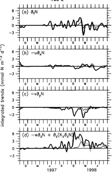
O• I I I I I I I I I [ • I [ . to

understand

the

main

processes

controlling

the

nitrate

/J••••,•

_ changes

to

understand

what

causes

new

production

variations.

50--1

_{_4.,---/._•/-"-'•••}

••__

In

_budget

order

_in

to

_the

examine

_euphotic

the

_layer,

temporal

_the

_nitrate

evolution

_tendency

of

_terms

the

nitrate

_have

100

••./5•/

//_/.x,•.-•

--_--:--

been

integrated

over

the

surface

layer

and

the

subsurface

150 .L--'•-•••q

•"////•'•/•//.•.•

advection,

and

vertical

processes

(vertical

advection

plus

(e) June 1998

50

• 2.0

o) 165

E

•oo

150

_{• I • • I • •}

q.,...•.

_{• ,}

_{• •}

_•

• 0.5

_{c o.o}

New production in the euphotic layer is compared to new production integrated in the upper 40 m (surface layer), and between 40m and the bottom of the euphotic layer (subsurface layer) at 0 ø, 165øE (Figure 10a) and 0 ø, 140øW (Figure 10b).

West of the biological front, the surface layer is nitrate depleted (Figure 8b). As nitrate is the limiting nutrient in the surface layer, new production occurs largely in the subsurface layer where nitrate is available (Figure 8c) and light is still sufficient. This situation is characteristic of oligotrophic

waters [Navarette, 1998] and results in low new production in

D M d S D M d

ß

_• 2.0 --

(b) 140øW

--

• 0.5--

_--

Figure 10. Time series of the modeled new production

(retool

N m

-2 d -•) at (a) 165øE

and (b) 140øW.

The thick line

is the new production in the euphotic layer, the thin line is the

new production in the upper 40 m, and the dotted line is the new production between 40 m and the base of the euphotic layer. A 5 ø zonal moving window averaging and a seven time step (35 days) Harming filter have been applied.

150øE 180 ø 150øW 120øW 90øW

Figure 9. Vertical sections of modeled monthly mean nitrate

concentration (gM) along the equator. Contour interval is 1

26,892

RADENAC

ET AL.: EL NIfO IMPACT ON EQUATORIAL

PACIFIC NITRATE