HAL Id: hal-01730772
https://hal.inria.fr/hal-01730772
Submitted on 13 Mar 2018
HAL is a multi-disciplinary open access
archive for the deposit and dissemination of
sci-entific research documents, whether they are
pub-lished or not. The documents may come from
teaching and research institutions in France or
L’archive ouverte pluridisciplinaire HAL, est
destinée au dépôt et à la diffusion de documents
scientifiques de niveau recherche, publiés ou non,
émanant des établissements d’enseignement et de
recherche français ou étrangers, des laboratoires
Towards a self-adaptive parameterization for
aerodynamic shape optimization
Régis Duvigneau, Badr Abou El Majd, Jean-Antoine Desideri
To cite this version:
Régis Duvigneau, Badr Abou El Majd, Jean-Antoine Desideri. Towards a self-adaptive
parameteriza-tion for aerodynamic shape optimizaparameteriza-tion. ESAIM: Proceedings, EDP Sciences, 2007. �hal-01730772�
Towards a self-adaptive parameterization
for aerodynamic shape optimization
R´
egis Duvigneau
Badr Abou El Majd
Jean-Antoine D´
esid´
eri
Introduction
In parametric shape optimization, a geometrical shape representation has to be chosen a priori, such as the use of B´ezier curves for instance. This task is called parameterization. This choice determines a subspace in which the search of the optimum shape is performed. This strategy has several advantages, such as:
• the reduction of the dimension of the problem, that is mandatory for stochastic optimization for instance ;
• the control of the smoothness of the shapes, that is necessary for numerical calculations and most realistic applications.
However, this strategy drastically reduces the set of shapes that can be reached by the optimization procedure. Then, the optimum shape found usually de-pends on the parameterization. The use of a parameterization that is not well adapted to the optimization problem can yield a low fitness optimum shape. Hence, in order to reduce this critical dependency, a self-adaptive parameter-ization methodology is developed, that adapts an initial and perhaps na¨ıve parameterization to the problem studied, on the basis of a first approximation of the optimum shape.
1
Self-adaptive parameterization
1.1
B´
ezier curve
One proposes to modify some characteristics of the parameterization to adapt it to the particular problem studied. For instance, consider an airfoil shape described by a B´ezier curve:
P(t) = n X i=0 Bin(t)Pi, (1) where t ∈ [0, 1] and {Bi
n}i=0,...,nare the Bernstein polynomials of degree n. The
during the optimization procedure. Since an airfoil is a rather thin body, only ordinates {yi}i=0,...,n are usually taken into account during the optimization,
whereas abscissae {xi}i=0,...,n are frozen. Then, one proposes to consider the
abscissae {xi}i=0,...,n as adaption variables that can be used to control the
characteristics of the parameterization[3].
Initially, the abscissae {xi}i=0,...,n can be uniformly distributed. Once a first
approximation of the optimum shape has been found by modifying the ordinates {yi}i=0,...,n, new abscissae {xi}i=0,...,n are defined, that are better adapted to
the problem, before a second optimization step is carried out. Actually, the ab-scissae are defined in such a way that an adaption cost functional is minimized, that measures the uneffectiveness of the current parameterization, with the con-straint that the current shape remains unaltered. This concon-straint is introduced to benefit from the optimization path already performed.
For a given set of abscissae {xi}i=0,...,n, consider the ordinates {yi}i=0,...,n
for which the shape is the least-squares approximation of the current shape. Then, the new abscissae {xi}i=0,...,n are chosen in order to minimize the total
variation of the corresponding ordinates {yi}i=0,...,n:
T V({yi}) = n X i=1 |yi− yi−1| ≈ Z 1 0 |y′(t)|dt, (2)
where y(t) is interpolating the control points. This criterion is introduced to regularize the control points polygon. This choice is justified by the fact that the optimization process yields a highly irregular control points polygon[2].
1.2
Free-Form Deformation (FFD)
For complex three-dimensional problems, such as those encountered in aero-dynamics, the Free-Form Deformation (FFD) approach[6] is adopted. It con-sists in defining a lattice embedding the shape and a local coordinate system (ξ, η, ζ) ∈ [0, 1] × [0, 1] × [0, 1] attached to this lattice. Then, the displacement of a point q inside the lattice is described by a third-order B´ezier tensor product:
∆q = ni X i=0 nj X j=0 nk X k=0 Bnii (sq)Bnjj (tq)Bknk(uq)∆Pijk, (3)
where (sq, tq, uq) results in a mapping of the coordinates (ξq, ηq, ζq) of q in the
lattice. Usually, this mapping is defined as the identity. The weighting coef-ficients ∆Pijk are considered as design variables. Finally, the FFD approach
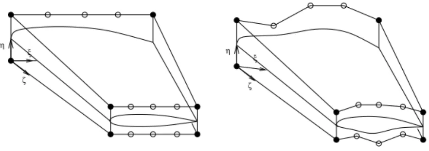
allows an easy deformation of an object, regardless of the representation of this object. Figure (1) depicts the FFD lattice built around a wing and figure (2) shows the deformation resulting from a control points displacement (plain mark-ers correspond to frozen control points whereas empty markmark-ers are control points moving vertically).
One proposes to consider the mapping that produces (sq, tq, uq) from the
η ζ
ξ
Figure 1: Initial FFD lattice.
η ζ
ξ
Figure 2: Deformed FFD lattice.
for each direction using the Bernstein polynomials basis :
s= φ(ξ) t= ψ(η) u= θ(ζ). (4) φ(ξ) = n′ i X i=0 Bn′i i (ξ)φi ψ(η) = n′ j X j=0 Bn ′ j j (η)ψj θ(ζ) = n′ k X k=0 Bn′k k (ζ)θk. (5)
Finally, weighting coefficients (φi)i=0,...,n′
i, (ψj)j=0,...,n′j and (θk)k=0,...,n′k are
considered as adaption variables. The adaption cost functional is inspired from the previous case (B´ezier curves) and measures the irregularity of the deforma-tion: JAD= 1 ninjnk ni X i=1 nj X j=1 nk X k=1 ∇δPijk ≈ Z 1 0 Z 1 0 Z 1 0 ∇δP(ξ, η, ζ) dξ dη dζ, (6) where δP (ξ, η, ζ) is interpolating the weighting coefficients. k∇δPijkk is the
Froebenius norm of the gradient tensor estimated over the elementary volume of indices ijk. The minimization of the adaption cost functional is subject to the constraint that the shape remains unaltered in a discrete least-squares sense. Thus, for a given mapping, the control points displacement is obtained by minimizing: JLS= N X n=1 1 2[∆q n new− ∆qoldn ] 2 δSn, (7) where ∆qn
newand ∆qoldn represent the displacements of the mesh node qnfor the
FFD deformations that correspond respectively to the new mapping and the cur-rent mapping. δSn is a weighting coefficient expressing the discrete integration
over the shape surface. Then, the adaption process consists in determining the adaption variables (φi)i=0,...,n′
i, (ψj)j=0,...,n′j and (θk)k=0,...,n′k to minimize the
2
Applications
2.1
Geometrical model problem
The proposed method is first applied to a geometrical problem arising from the calculus of variations[4]. It consists in reconstructing an arc by minimizing the following cost function:
JOP T =
pα
A, (8)
where α > 1 is a positive real number. p and A are the pseudo-length of the arc and the pseudo-area below the arc, defined by:
p= Z 1 0 p x′2(t) + y′2(t)ω(t)dt A = Z 1 0 y(t)x′(t)ω(t)dt. (9)
ω(t) is a positive and adjustable function. It was shown in [4] that given a shape for which y is a smooth function of x admitting one and only one extremum, α and ω(t) can be set uniquely so that JOP T is a unimodal function of y(t) (for
fixed x(t)) and its unique minimum is realized by the given shape.
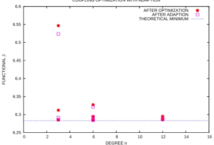
The shape optimization procedure including the adaption method is applied to this problem[3]. Here, α and ω(t) are chosen in such a way that the solution corresponds to a circular arc (α = 2 and ω(t) = 1), for which the theorical minimum value is 2Π. The arc is successively parameterized by B´ezier curves of increasing degrees. The cost function values obtained with respect to the degree are depicted in figure (3).
6.25 6.3 6.35 6.4 6.45 6.5 6.55 6.6 0 2 4 6 8 10 12 14 16 FUNCTIONAL J DEGREE n
COUPLING OPTIMIZATION WITH ADAPTION
AFTER OPTIMIZATION AFTER ADAPTION THEORETICAL MINIMUM
Figure 3: Results for the model problem : cost function values obtained af-ter a single optimization and then afaf-ter adaption+optimization, for different parameterization degrees.
Using a curve of degree 3 whose control points abscissae are uniformly dis-tributed, poor results are obtained after a single optimization (about 6.55). This value is slightly decreased after adaption thanks to the least-squares fitting. A second optimization using the adapted parameterization yields a significant im-provement (about 6.31). If a third adaption + optimization step is performed, a cost function value very close to the theorical minimum is obtained. Similar results are observed using a curve of higher degree. These results show that an adapted parameterization of degree 3 allows to reach a shape of better fitness than a na¨ıve parameterization of degree 6 or even 12.
2.2
Aerodynamic shape optimization
The proposed method is now faced with the aerodynamic optimization of the shape of a wing of a business aircraft[1] (courtesy of Piaggio Aero Ind.). The compressible flow is modeled by the Euler equations, which are solved using a finite-volume approach on unstructured meshes. The shape deformation is parameterized using the FFD approach described above. Figure (1) shows the wing shape embedded in the FFD lattice. The optimization procedure relies on the Multi-directional Search Algorithm (MSA) from Torczon[7], which is a derivative-free method similar to the well-known Nelder-Mead simplex method, but designed for parallel computations. The aim of the optimization is the reduction of the drag, including a constraint on the lift.
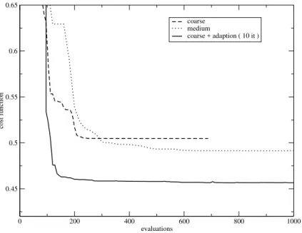
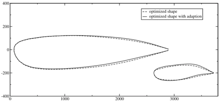
Optimization exercises are carried out using a coarse parameterization (8 d.o.f.), a medium one (20 d.o.f.) and a fine one (32 d.o.f.), with and without adaption. For the tests with adaption, the parameterization adaption procedure is performed every ten iterations, yielding a regular parameterization update until convergence of both optimization and adaption procedures. This strategy promotes the avoiding of local minima. Figure (4) shows the evolution of the cost function using a coarse parameterization with and without adaption and a medium parameterization without adaption. As can be observed, the use of the adaption procedure yields a faster convergence towards a shape of better fitness. Finally, the use of a coarse but adapted parameterization is more effective than the use of a medium but na¨ıve one. The results obtained using a medium parameterization (figure (5)) exhibit the same behavior. The optimum shapes found using the initial parameterization and the adapted parameterization are depicted in figure (6). As can be observed, the fitness improvement thanks to adaption corresponds to very slight modifications of the shape.
3
Conclusion
A self-adaptive parameterization methodology for shape optimization has been developed. It relies on the regularization of the design variables subject to the constraint that the shape remains unaltered in a least-squares sense. Its efficiency has been demonstrated for a geometrical model problem using B´ezier curves, and then for the aerodynamic shape optimization of a wing using the
0 200 400 600 800 1000 evaluations 0.45 0.5 0.55 0.6 0.65 cost function coarse medium coarse + adaption ( 10 it )
Figure 4: Evolution of the cost function with and without adaption using a coarse parameterization. 0 500 1000 1500 2000 2500 3000 evaluations 0.45 0.5 0.55 0.6 0.65 cost function medium fine medium + adaption ( 10 it )
Figure 5: Evolution of the cost function with and without adaption using a medium parameterization.
0 1000 2000 3000 -400 -200 0 200 400 optimized shape optimized shape with adaption
Figure 6: Comparison of the shapes obtained (root and tip section).
FFD approach.
The strong influence of the parameterization on the results has clearly be established. The use of the proposed adaption procedure has increased the convergence rate and improved the fitness of the shape found.
References
[1] M. Andreoli, A. Janka, and J.-A. D´esid´eri. Free-form deformation param-eterization for multilevel 3D shape optimization in aerodynamics. INRIA Research Report 5019, November 2003.
[2] J.-A. D´esid´eri. Two-level ideal algorithm for parametric shape optimization. Journal of Numerical Mathematics, 14, 2006.
[3] J.-A. D´esid´eri, B. Abou El Majd, and A. Janka. Nested and self-adaptive b´ezier parameterization for shape optimization. In International Confer-ence on Control, Partial Differential Equations and Scientific Computing, Beijing, China, September 13-16 2004.
[4] J.-A. D´esid´eri and J.-P. Zol´esio. Inverse shape optimization problems and application to airfoils. Control and Cybernatics, 34(1), 2005.
[5] R. Duvigneau. Adaptive parameterization using free-form deformation for aerodynamic shape optimization. INRIA Research Report RR-5949, July 2006.
[6] T.W. Sederberg and S.R. Parry. Free-from deformation of solid geometric models. Computer Graphics, 20(4):151–160, 1986.
[7] V. Torczon. Multi-Directional Search: A Direct Search Algorithm for Parallel Machines. PhD thesis, Houston, TX, USA, 1989.