An application of advanced statistical techniques to forecast the demand for air transportation

FLIGHT TRANSPORTATION LABORATORY DEPARTMENT OF AERONAUTICS AND ASTRONAUTICS

MASSACHUSETTS INSTITUTE OF TECHNOLOGY

FTL Report R77-3 August 1977

AN APPLICATION OF ADVANCED STATISTICAL TECHNIQUES TO FORECAST THE DEMAND FOR AIR TRANSPORTATION

DENNIS F. X. MATHAISEL NAWAL K. TANEJA

TABLE OF CONTENTS

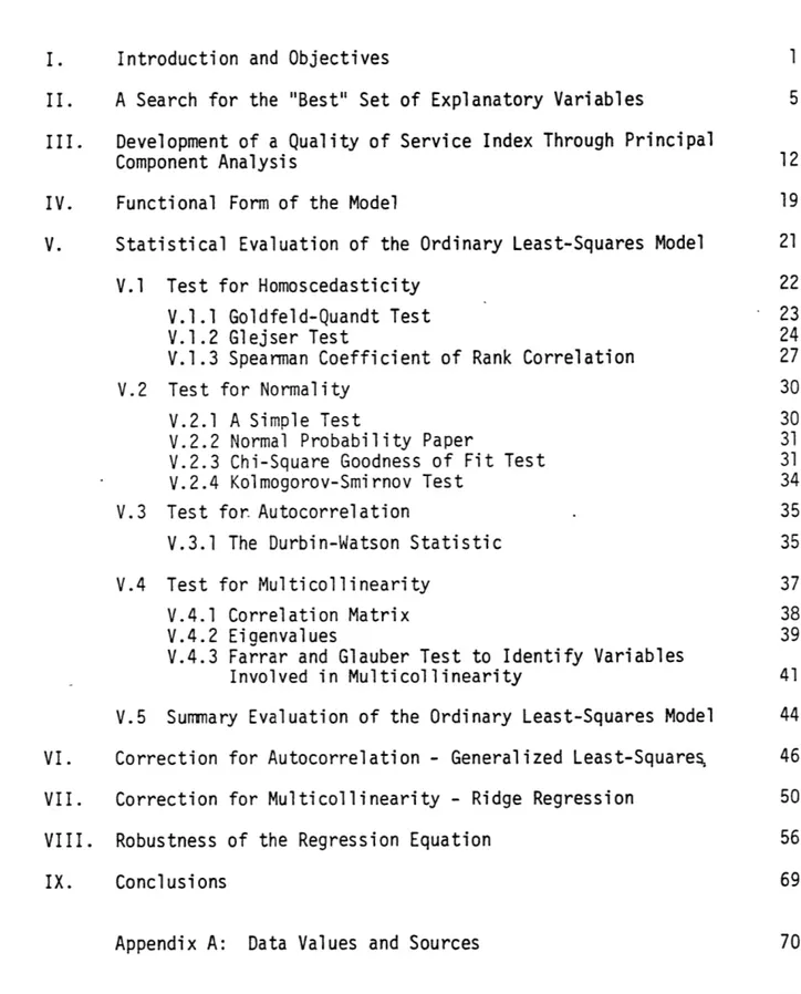
I. Introduction and Objectives 1

II. A Search for the "Best" Set of Explanatory Variables 5 III. Development of a Quality of Service Index Through Principal

Component Analysis 12

IV. Functional Form of the Model 19

V. Statistical Evaluation of the Ordinary Least-Squares Model 21

V.1 Test for Homoscedasticity 22

V.1.1 Goldfeld-Quandt Test 23

V.1.2 Glejser Test 24

V.1.3 Spearman Coefficient of Rank Correlation 27

V.2 Test for Normality 30

V.2.1 A Simple Test 30

V.2.2 Normal Probability Paper 31

V.2.3 Chi-Square Goodness of Fit Test 31

V.2.4 Kolmogorov-Smirnov Test 34

V.3 Test for Autocorrelation 35

V.3.1 The Durbin-Watson Statistic 35

V.4 Test for Multicollinearity 37

V.4.1 Correlation Matrix 38

V.4.2 Eigenvalues 39

V.4.3 Farrar and Glauber Test to Identify Variables

Involved in Multicollinearity 41

V.5 Summary Evaluation of the Ordinary Least-Squares Model 44 VI. Correction for Autocorrelation - Generalized Least-Square!, 46 VII. Correction for Multicollinearity - Ridge Regression 50 VIII. Robustness of the Regression Equation 56

IX. Conclusions 69

Appendix A: Data Values and Sources 70

I. Introduction and Objectives

For some time now regression models, often calibrated using the ordinary least-squares (OLS) estimation procedure, have become common tools for

forecasting the demand for air transportation. However, in recent years more and more decision makers have begun to use these models not only to

forecast traffic, but also for analyzing alternative policies and strategies. Despite this increase in scope for the use of these models for policy analysis,

few analysts have investigated in depth the validity and precision of these models with respect to their expanded use. In order to use these models

properly and effectively it is essential not only to understand the

under-lying assumptions and their implications which lead to the estimation procedure, but also to subject these assumptions to rigorous scrutiny. For example,

one of the assumptions that is built into the ordinary least-squares estimation technique is that the explanatory variables should not be correlated among themselves. If the variables are fairly collinear, then the sample variance of the coefficient estimators increases significantly, which results in

inaccurate estimation of the coefficients and uncertain specification of the model with respect to inclusion of those explanatory variables. As a

correc-tive procedure, it is a common practice among demand analysts to drop those explanatory variables out of the model for which the t-statistic is insigni-ficant. This is not a valid procedure since if collinearity is present the

increase in variance of the coefficients will result in lower values of the t-statistic and rejection from the demand model of those explanatory

variables which in theory do explain the variation in the dependent variable. Thus, if one or more of the assumptions underlying the OLS estimation pro-cedure are violated, the analyst must either use appropriate correction

procedures or use alternative estimation techniques.

The purpose of the study herein is three-fold: (1) develop a "good" simple regression model to forecast as well as analyze the demand for air transportation; (2) _{using this model, demonstrate the application of various statistical tests} to evaluate the validity of each of the major assumptions underlying the OLS estimation procedure with respect to its expanded use of policy analysis; and,

(3) demonstrate the application of some advanced and relatively new statistical estimation procedures which are not only appropriate but essential in eliminating

the common problems encountered in regression models when some of the under-lying assumptions in the OLS procedure are violated.

The incentive for the first objective, to develop a relatively simple single equation regression model to forecast as well as analyze the demand for air

transportation (as measured by revenue passenger miles in U.S. Domestic trunk opera-tions), stemmed from a recently published study by the U.S. Civil Aeronautics

Board [CAB, 1976]. In the CAB study a five explanatory variable regression equation was formulated which had two undesirable features. The first was the inclusion of time as an explanatory variable. The use of time is un-desirable since, from a policy analysis point of view, the analyst has no "control" over this variable, and it is usually only included to act as a proxy for other, perhaps significant, variables inadvertently omitted from the equation. The second undesirable feature of the CAB model is the "delta log" form of the equation (the first difference in the logs of the variables),which allowed a forecasting interval of only one year into the future. This form was the result of the application of a standard correc-tion procedure for collinearity among some of the explanatory variables.

In view of these two undesirable features, it was decided to attempt to improve on the CAB model. In addition to the explanatory variables consi-dered in the CAB study a number of other variables were analyzed to deter-mine their appropriateness in the model. Sections II and III of this report describe the total set of variables investigated as well as a method for searching for the "best" subset. Then, Section IV outlines the decisions involved in selecting the appropriate form of the equation.

The second objective of this study is to describe a battery of statistical tests, some common and some not so common, which evaluate the validity of each of the major assumptions underlying the OLS estimation procedure with respect to single equation regression models. The major assumptions assessed

in Section V of this report are homoscedasticity, normality, autocorrelation, and multicollinearity. The intent here is not to present all of the statistical

tests that are available, for to do so would be the purpose of regression textbooks, but to scrutinize these four major assumptions enough to remind the analyst that it is essential to investigate in depth the validity and precision of the model with respect to its expanded use of policy analysis. It is hopeful that the procedure outlined in this report sets an example to demand modeling analysts of the essential elements used in the development of reliable forecasting tools.

The third and ultimate objective of this work is to demonstrate the use of some advanced corrective procedures in the event that any of the four above mentioned assumptions have been violated. For example, the problem

of autocorrelation can be resolved by the use of generalized least-squares(GLS), which is demonstrated in Section VI of this report; and the problem of

multi-collinearity , usually corrected by employing the cumbersome and restrictive delta log form of equation, has been eliminated by using Ridge regression (detailed in Section VII). Finally, in Section VIII an attempt is made to determine the "robustness" of a model by first performing an examination of the residuals using such techniques as the "hat matrix", and second by the application of the recently developed estimation procedures of Robust

regression. Although the techniques of Ridge and Robust regression are still in the experimental stages, sufficient research has been performed to warrant their application to significantly improve the currently operational regression models.

5

II. A Search for the "Best" Set of Explanatory Variables

One criterion for variable selection was to find that minimum number of independent variables which maximize the prediction and control of the dependent variable. The problem is not one of finding a set of indepen-dent variables which provides the most control for policy analysis, or those variables which best predict the behavior of the dependent variable, but, rather, constraining the number of these variables to a minimum. The hazards of using too many explanatory variables are widely known: an inevi-table increase in the variance of the predicted response [Allen,1974]; a more difficult model to analyze and understand; a greater presence of highly intercorrelated explanatory variables; a reduction in the number of degrees of freedom; and a more expensive model to maintain since the value of each explanatory variable must also be predicted.

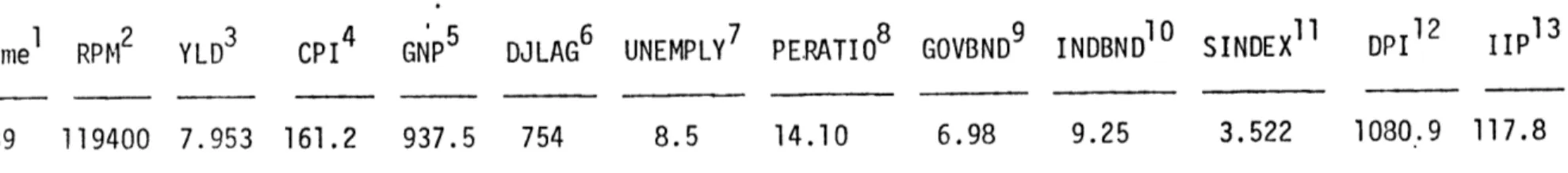
Initiallyten explanatory variables were selected for analysis based partly on the study by the Civil Aeronautics Board [CAB, 1976]. These variables are:

(1) TIME - included to provide for any trend resulting from variables omitted from the model.

(2) YLD = Average scheduled passenger yield - total domestic passenger revenues plus excess baggage charges and applied taxes divided by scheduled revenue passenger miles. The yield is deflated by the consumer price index to arrive at the real cost per mile to the consumer.

(3) GNP = Gross National Product, expressed in real terms (1967 dollars) to measure changes in purchasing power.

(4) DJLAG = Dow Jones Industrial Average , lagged by one year, computed from the quarterly highs and lows of the Dow "30" price range. (5) UNEMPLY = Unemployment - percent of the civilian labor force.

(6) PERATIO = Price to Earnings Ratio - ratio of price index for the last day of the quarter to quarterly earnings (seasonally adjusted annual rate). Annual ratios are averages of quarterly data.

(7) GOVBND or INDBND = Bond Rate - both U.S. Government bond yields and industrial bond yields were studied.

(8) DPI = Disposable Personal Income. (9) IIP = Index of Industrial Production.

(10) SINDEX = Quality of Service - an index obtained by principal compo-nent analysis of five variables: total available seat miles, average overall flight stage length, average on-line passenger trip length,

average available seats per aircraft, and average overall airborne speed. The index is used as a measure of the improvement in the quality of service offered. (See Section III).

The data values and sources for these ten variables are given in Table 1 (Appendix A).

The problem then is how to shorten this list of independent variables so as to obtain the "best" selection - "best" in the sense of maximizing prediction and control based on a model which is appropriate not only on theoretical grounds but which can also be calibrated relatively easily. As a start, the variables should be screened before-hand in some systematic way. They should make theoretical sense in the regression equation, and

they should meet the more important characteristics such as (1) measurabi-lity, (2) consistency, (3) reliability of the source of the data,

(4) accuracy in the reporting of the data, (5) forecastability, and (6) controlability - that is, at least some of the variables should be under your control.

Then, to aid the investigator in his selection, automatic statistical search procedures are available (see Hocking [1972]). One such search procedure calls for an examination of all possible regression equations1 involving the candidate explanatory variablesand selection of the "best" equation according to some simple criterion of goodness of fit. In this study a statistical measure of "total squared error" was utilized as a criterion for selecting independent variables.2 This statistic, given by Mallows [1964],has a bias component and a random error component.

The total squared error (bias plus random) for n data points, using a fitted equation with p terms (including bo) is given by:

r n n

TM1 -i)2 + ~ 2(9 (A.1

i=1 i=1

bias random error component* component where: v = E [Y.] according to the true relation

nI = E [Y ] according to the fitted equation a 2(' ) = variance of the fitted value Y.

a2 = true error variance.

Note that the all possible regression equations search procedure pre-supposes that the functional form of the regression relation has already been established. Both the additive form and the multiplicative form were evaluated simultaneously. The multiplicative form (or log model) was our final choice, so it will be represented here. See Section IV. 2 Other statistical selection criteria include step-wise regression,

R 2_{, MSEP}

, and t-directed search. See Neter and Wasserman [1974]. pp

With a good unbiased estimate of o2_{(call it a2) it}

can be shown [Daniel and Wood, 1971 ; Gorman and Tomau, 1966] that the statistic C _{is an estimator of}

_rP:

C = SSEP - (n-2p) _(11.2)

where SSE stands for the sum of squares due to error.

When there is _{negligible bias in a regression equation (i.e. sum of} squares due to bias, SSB, is zero) the C statistic has an expected value of p:

E[C pSSBP = 0] = p (11.3)

Thus, when the C values for all possible regressions are plotted against p, those equations with negligible bias will 'tend to cluster about the line Cp = p. Those equations with substantial bias will tend to fall above the line. Since bias is due to variables omitted from the equation, adding terms

may reduce the bias but at the added expense of an increase in the variance of the predicted response. The trade-off is accepting some bias in order to get a lower average error of prediction. The dual objective in this study, maximum prediction with a minimum number of variables, now becomes clear. Therefore, the object was to find that set of explanatory variables that

leads to the smallest Cp value. If that set s-hould contain substantial bias another set may be preferred with a slightly larger C which does not contain substantial bias.

The Cp values for all possible regressions were calculated on the UCLA BMD09R regression series computer program, and are plotted against p in Figure A. The C value for point A is the minimum one, and appears to contain negligible bias. Equations represented by points B and C and surrounding points are also potential candidates, although point B does contain some small bias, and at point C the number of variables has

increased by one.

From a purely statistical point of view, the equation represented by point A in Figure A (containing the five explanatory variables TIME, YLD, DJLAG, IIP, SINDEX) appears to represent the "best" set of independent variables. But, the solution is unique to the C statistical criterion, and therefore may be "best" only in terms.of this criterion. Not all of the statistical procedures for variable search (R2 criterion, MSE criterion, foreward/backward stepwise regression, or t-directed search) may lead to the same conclusion. Indeed each procedure has its unique solution, and the conclusions are only valid for our sample data. Further-more, the importance of subjective evaluation can not be overlooked.

Consider the model chosen on the basis of minimum Cp criterion:

ln RPM=b₀ + b1 ln TIME + b2 In YLD + b3 ln DJLAG + b4 in IIP +b 5 ln SINDEX (11.4) There is no control over the variable TIME. In fact, as is often typical in time series data, this variable is merely a surrogate for those variables omitted from the regression equation and some which are included in the equation. There is also no control over the Dow Jones index, DJLAG, and there is some question as to whether this variable can be forecasted

liably. The index of industrial production variable, IIP, is supposed to measure changes in the economy and relate them to the growth in air travel, but it is only a measure of the industrial or business economy. It does not reflect changes in personal spending. Since the attempt in this study is to develop an aggregate model of air travel demand, it would be more appropriate to employ an aggregate measure of the economy - for

example, GNP.

What remains after this pragmatic investigation is the following selected relationship:

ln RPM = b 0 + b 1 ln YLD + b2 ln GNP + b3 ln SINDEX (11.5)

The number of explanatory variables has been reduced considerably and yet the analyst still remains in control over two of them - YLD and SINDEX. The first variable, YLD, tracks changes in the cost of air travel; the second variable, GNP, measures changes in passenger traffic associated with changes in the national economy; and the third variable, SINDEX,

is an indicator of the service offered by the industry. Thus, the objectives in the variable selection process appear to be met:

- the number of variables have been kept to a bare minimum;

- the variables make theoretical sense in the regression equation; - the variables are measurable, consistent, reliable, accurate,

forecastable, and, with the exception of GNP, controlable, that is, under the control of the policy decision maker.

III. Development of a Quality of Service Index Through Principal Component Analysis

An important measure which should be included in the economic modeling of the growth of air transportation is the quality of service offered. The

level of service tends to propagate the level of air travel: that is, as the quality of air service increases, demand increases. Suppose one was

to represent the improvement in the quality of air service through the

following variables.

- average available seats per aircraft (SEATS) - average overall airborne speed (SPEED)

- average on-line passenger trip length (PTL) - average overall flight stage length (FSL) - total available seat miles (ASM)

If the classical supply and demand equation economic modeling principle was to be employed it would be possible to design a demand equation expres-sing RPM as a function of the quality of service,

RPM = f1(Quality of Service,...),

and a supply equation expressing the quality of service as a function of

the above five variables,

Quality of Service = f2(SEATS,SPEEDPTL,FSL,ASM).

In this way adding an additional equation to form a simultaneous equation model allows for a complex interaction within the system conjoining the

demand and supply variables. This interaction, however, is undesirable for the following reasons. First, by nature of the simultaneous equation speci-fication, the quality of service variable will be in a dynamic state. The

demand and quality of service will be allowed to interact with each other in two-way causality. Although its cause and effect role is different in the two equations, the quality of service variable is still considered to be endogenous due to its dependent role. In the present model speci-fication,for simplicity,it was decided to represent the improvement in quality of service in a static state with causality in only one direction. Second, in a simultaneous equation model it is necessary to "identify" the quality of service function (in terms of total travel time, for example). Yet, since this is an aggregate model of air transportation demand without

regard to length of haul or nature of travel (business, pleasure, personal, etc.), it would be incorrect to specify the quality of service offered in

such terms as total travel time or total frequency available. Third, a simultaneous equation model is more complex than.a single equation speci-fication, which makes such a model more difficult to control and interpret - incongruous to the objective of developing a simple model. Fourth, a supply equation cannot be designed for level of service from the five variables listed since at least one of the variables, total available seat miles, is itself a supply variable. Thus, while on theoretical grounds it may be argued that the dual-equation specification is more appropriate,

the intention is to be crude because the focus here is on the estimation procedures rather than the theoretical specification.

Therefore, the objective in this study of an aggregate travel demand model is not to construct a supply equation for use in a simultaneous

equation model, but rather to design one factor which can be used as a proxy for the quality of service in a single equation model. Principal component analysis (PCA) [Bolch & Huang, 1974; Davis, 1973] takes the five

variables mentioned above, and makes a linear combination of them in such a manner that it captures as much of the total variation as possible. This linear combination, or principal component, will serve as a proxy for

level of service.

Before discussing the development of the principal component analysis technique, it will be difficult to understand the meaning of the linear combination of the five variables unless they are all measured in the same

units (the raw data is given in Table 2,Appendix A). A linear combination of seats, miles and miles-per-hour is at best unclear. Therefore, before computing

the components it is possible to convert the variables to standard scores, or z-scores,

Z =x-

x

s

(where: X is the sample mean, ands is the sample standard deviation), which are pure numbers, and the problem of forming linear combinations of different measurements vanishes.

From the standard scores of m variables it is possible to compute an m x m matrix of variances and covariances. (The variance-covariance matrix of the z-scores for the five variables is simply the correlation matrix of the original data set. This is given Table 3.) From this,one can extract m eigenvectors and m eigenvalues. Recall that elements in an m x m matrix can be regarded as defining points lying on an m-dimensional ellipsoid. The eigenvectors of the matrix yield the principal axes of the ellipsoid, and the eigenvalues represent the lengths of these axes. Because a variance -covariance matrix is always symmetrical, these m eigenvectors will be

orthogonal, or oriented at right angles to each other. Figure B illustrates this principle graphically for a two-dimensional matrix.

Table 3

Variance-Covariance Matrix of the z-scores of the Five

Quality of Service Variables

ASM ASM FS L PTL 1.0 0.975 0.923 FSL 0.975 1.0 PTL 0.923 0.909 SEATS 0.966 0.933 SPEED 0.934 0.954 0.909 1.0 0.975 SEATS 0.966 0.933 0.975 1.0 SPEED 0.934 0.954 0.878 0.913 0.878 0.913 1.0

Principal Axes of a 2-Dimensional Ellipsoid

X

₂ I a b II Figure B

Vectors I and II are the eigenvectors, and segments a and b are the cor-responding eigenvalues. This is the case where X and X2 are positively correlated. As the correlation between the two variables increases, the ellipse more closely approaches a straight line. In the extreme case if X and X2 are perfectly positively correlated, the ellipse will degenerate into a straight line. It is not possible to demonstrate the 5-dimensional variance-covariance matrix graphically, but it can be envisioned in the same manner. The eigenvectors and eigenvalues of this 5-dimensional vari-ance-covariance matrix can be computed easily and are shown below.

0.985 0.041

-0.980

0.139

1

0.962 II -0.251

0.983

-0.151

0.960 0.222 I Eigenvalue = 4.7447 II Eigenvalue = 0.1563

-0.147

-0.062

0.042

-0.085

0.111

-0.031

I = 0.073 IV = 0.079 V = 0.026

0.001 -0.093 -0.046

L0. 164 -:0.033J 0.010j

III Eigenvalue = 0.0613 IV Eigenvalue = 0.0321 V Eigenvalue = 0.0057 The total of the five eigenvalues is

4.7447 + 0.1563 + 0.0613 + 0.0321 + 0.0057 = 5.0

which is equal to p, or the number of variables. This is also equivalent to the trace of the variance-covariance matrix for the z-scores. Thus, the sum of the eigenvalues represents the total variance of the data set. Note that the first eigenvalue accounts for 4.7447/5.0 = 94.89 percent of the trace. Since the eigenvalues represent the lengths of the principal axes of an ellipsoid, then the first-principal axis, or principal component, accounts for 94.89 percent of the total variance. In other words, if one measures the variation in the data set by the first principal component, it accounts for almost 95 percent of the total variation in the observations. Principal components, therefore, are nothing more than the eigenvectors

of a variance-covariance matrix.

Principal components are also a linear combination of the variables, X, of the data set. Thus

Y = 6lX + + 63X3 + 64X4 + 65X5

is the first principal component, and the 's are the elements of the first eigenvector. If one were to use the standard scores in lieu of actual data, the first principal component becomes:

** * * *

*

where the coefficients 6 are the elements of the eigenvectors corresponding to the standardized variance-covariance matrix. Transforming this equation in terms of the original data, Z =X -X , and substituting in the

ele-5 *

ments of the standardized eigenvectors, S , for the first principal

com-ponent, the level of service index can be computed as follows:

Level of Service Index

=

0.985

ASM

88.

.103

+0.980 FSL

-

282.417

95.709 +0.962 PTL - 585.4

81.237

+0.983 SEATS - 77.15 33.375 +0.960 'SPEED

_84.987

- 290.433

Therefore, this procedure results in a new set of data, termed the principal component (or factor) scores, which is a linear combination of the five level of service variables and accounts for 95 percent of the variation in the observations. The centered principal component scores are given in Table 2. To these scores the quantity 2.0 is subsequently added, which is the minimum positive integer required to transform the scores to all positive values for use in a logarithmic model. The result-ing specified index, termed SINDEX, is the proxy for the quality of service offered.

IV. Functional Form of the Model

Two functional forms were investigated: the additive form, Y = 0 + IxI + 2

x2

+ ... + nXn + C

and the multiplicative form,

Y = 0X 1 -0X 26 2 * xn .:

The multiplicative form is

in

a class of models called intrinsically linear

models because it

can be made linear through a logarithmic transformation

of the variables:

* *

ln Y =0 + 1 In X + in

l2

X2 + ... + n ln X +

* *

where, 60 and e are the logarithmic transformations of the constant and the error term.

The delta log model,

ln Y-

1n

Y

t-1

+ S (In Xlt - ln X1t 1) +

which is commonly used because it tends to eliminate the multicollinearity - and serial correlation problems,was not employed because it removes the

secular trend in

the data and only allows one to forecast out one period

- not really suitable for long-term forecasting.

Both the additive form and the multiplicative form (or logarithmic model) were evaluated while the variable selection process was taking place

(see Section

II

). This was necessary since the automatic variable selec-tion technique that was used, Mallows C criterion, required that the

for the functional form. This conclusion was reached after an exhaustive and extensive evaluation of both forms during the variable selection process. To illustrate this conclusion compare the statistics of both forms using the three explanatory variables which were finally selected. Additive Model

RPM = -56.556 + 0.934 YLD + 0.068 GNP + 28.130 SINDEX (0.281) (1.252) (2.914)

R2 = 0.9780

Standard Error of Estimate = 6.1536

n = 27

Natural Logarithm Model

ln RPM = 7.433 - 0.735 ln YLD + 0.592 ln GNP + 1.132 ln SINDEX (-3.443) (1.934) (7.810)

R2 = 0.9968

Standard Error of Estimate = 0.0534 n = 27

The figures in paratheses are the corresponding t-ratios. Not only is the sign of the coefficient for yield in the additive model "wrong" (the plus sign of the coefficient infers that as the 'cost of travel in-creases the amount of travel increases!), but it is difficult to place any confidence in either its coefficient or that of GNP since the t-ratios are not significant.

V. Statistical Evaluation of the Ordinary Least Squares Model In the development of an econometric air travel demand model, such as Y = X6 + c, the analyst attempts to obtain the best values of the parameters 6 given by estimators b. The method of ordinary least-squares produces the best estimates in terms of minimizing the sum of the squared residuals. The term "best" is used in reference to certain desired properties of the estimators. The goal of the analyst is to select an estimation procedure which produces estimators (for example price elasticity of demand) which are unbiased, efficient, and

consis-tent [Wonnacott & Wonnacott, 1970]. The method of least-squares estima-tion is used in regression analysis because these properties can be achieved if certain assumptions can be made with respect to the distur-bance term c and the other explanatory variables in the model. These assumptions are:

1. Homoscedasticity - the variance of the disturbance term is constant;

2. Normality - the disturbance term is normally distributed; 3. No autocorrelation - the covariance of the disturbance term

is zero;

4. No multicollinearity - matrix X is of full column rank.

This section goes through each of these assumptions performing various tests to determine if any assumption is violated. (For further reference on

each assumption see Taneja [1976]). Corrective procedures for the violations are explained and examined in subsequent sections of this report. The

ordinary least-squares regression equation which is to be tested is as follows:

ln RPM = 7.433 - 0.735 ln YLD + 0.592 in GNP + 1.132 in SINDEX (V.1)

(3.507) (-3.443) (1.934) (7.810)

R = 0.9968

Standard Error of Estimate = 0.0534 Durbin-Watson Statistic = 0.77 n = 27 observations

The figures in parentheses are the corresponding t - ratios.

V.1 Test for Homoscedasticity

The assumption of constant variance of the disturbance term is called homoscedasticity. When it is not satisfied, the condition is called heteroscedasticity. Heteroscedasticity is fairly common in the analysis of cross-sectional data. Air transportation demand models incorporating income distribution of air travelers, for example, usually encounter this problem because the travel behavior of the rich and poor can differ in the large and small variances of their spending pattern.

If all assumptions except the one related to homoscedasticity are valid, the estimators b produced by least-squares are still unbiased and consistent, but they are no longer minimum-variance estimators. The presence of hetero-scedasticity will distort the measure of unexplained variation, thus distort-ing the conclusions derived from the multiple correlation coefficient R and the t - statistic tests. The problem is that the true value of a hetero-scedastic residual term is dependent upon the related explanatory variables. Thus, the R and t-values become dependent on the range of the related explanatory variables. In general, the standard goodness-of-fit statistics will usually be misleading. The t and F distributed test statistics used for testing the significance of the coefficients will be overstated, and

the analyst will unwarily be accepting the hypothesis of significance

more often than he should.

V.1.1. Goldfeld-Quandt Test

A reasonable parametric test for the presence of heteroscedasticity is one proposed by Goldfeld and Quandt [1965]. The basic equation for n observations, Y =X + E, is partitioned in the form:

YAx A A

+A

YB B B (V.2)

The vectors and matrices with subscript A refer to the first n/2 observations, and those with subscript B refer to the last n/2 observations. If eA*

and eB represent the least-squares residuals computed for both sets of observations independently (from separate regressions),then the ratio e'AeA of the sum of squares of these residuals will be distributed as e'Be

B F(n/2 -p, n/2 - p). The null hypothesis is that the variance of

the disturbance term is constant, aA = B; that is, the data is homoscedastic. The null hypothesis will be rejected if the calculated F value exceeds

F(a _; nA _{-p, nB -'}

The calculated F value for the model shown in equation (V.1) is

F n , = F - SSEA/(13-4) A n 13-4, 14-4 SSEB /(4-4)

.0.012/9 0.008/10

which is less than F(.05,9,10) = 3.02. So, the null hypothesis that the data set is homoscedastic can be accepted .

Sometimes the variance of the disturbance term changes only very slightly and heteroscedasticity is not so obvious. To help exaggerate the differences in the variance Goldfeld and Quandt suggest the omission of about 20 percent of the central observations. The elimination of 20 per-cent of the data reduces the degrees of freedom, but it tends .to make the difference between e'AeA and e'BeB larger. Of the 20 total observations in the data base, the middle 6 observations were omitted. The calculated F value is F -= F -= SSEAI(10-4) nAp, nB~ F _{0 4}' 4 SSEB/(11-4) = .005/6 .005/7 = 1.167 (V.4)

which is _{less than F(.05,6,7)= 3.79. Again the null hypothesis that} the data set is homoscedastic can be accepted.

V.1.2 Glejser Test

This test ,due to Glejser [1969], suggests that decisions about homo-scedasticity of the residuals be taken on the basis of the statistical significance of the coefficients resulting from the regression of the abso-lute values of the least squares residuals on some function of X., where X

mean, for this example, considering fairly simple functions like:

(i)

lei

= b + b ln YLD (ii) lel = b + b ln GNP (iii)

jel

= b0 + b ln SINDEX

and testing the statistical significanc Two relevant possibilities may then ari scedasticity" when bo = 0 andb $0 ;

scedasticity" when _b 0 0 and b $0. Using the above relationships the

(i)

let

= 0.038 + (0.682) (ii) let = 0.080

-(o.641)

:e _{of the coefficients bo and} b1 . se: (1) the case of "pure and (2) the case of "mixed

hetero-regression equations are: 0.002 ln YLD

(0.073) 0.006 ln GNP

(-0.309)

(iii) le| = 0.044 - 0.004 ln SINDEX

(5.586) (-0.376)

The figures in parentheses are the corresponding t - ratios.

A test for deciding whether or not b = 0 or b = 0 is based on the t-statistic. The decision rule with this test statistic, when cofitrolling

the level of significance at a, is:

if |til < t(1 - a/2 ; n-2)., if It | > t(1 - a/2 ; n-2) ,.

then conclude b = 0, then conclude b

$

0. To draw inferences regarding both b₀ = 0 and b1 =0

jointly,

a test can be conducted which is based on the F-distribution (see Neter & Wasserman

[1974]). Define the calculated F-statistic as:

Fcalculated

n(b0 - S)2 + 2(EXi ) (bo - %) (b- + (EX2) (b1 - S)2

2 (MSE)

where 6 0,S. 1 0, and MSE is the mean square error. The decision rule with this F-statistic is:

if _Fcalculated < F(l - a; n-2), then conclude that b₀ = 0 and b= 0 jointly

At a 5 percent level of significance, where t(.975, 27-2) = 2.06

and F(.95, 2, 27-2) = 3.38, the results of the significance tests on b and b are the following:

For regresssion (i) :

Fcalculated = 27(0.038 |tol = 0.862 < 2.06 |til = 0.073 < 2.06 - 0)2 + 2(51.234)(0.038 - 0)(.002-0) + (98.118)(.002)2 2(.0075) = 3.127 < 3.38

which infer that b0 = 0, bI = 0, and both b and b1 are equal to

zero jointly. So neither pure nor mixed heteroscedasticity are associated with the variable ln YLD.

For regression (ii):

_it

₀

₁

_{= 0.641 < 2.06}

it

1

1

= 0.309 < 2.03 F calculated = 2.536 < 3.38

inferring that b = 0, b = 0, and both b0 and b1 are equal to zero jointly. So neither pure nor mixed heteroscedasticity are associated with ln GNP. For regression (iii):

to = 5.586 > 2.06 t= 0.376< 2.06

Fcalculated = 3.86 > 3.38

Although b0 is not equal to zero and the F-distributed statistic fails the test, bi

js

equal to zero- concluding once again that neither pure nor mixed heteroscedasticity are associated with the variable ln SINDEX.

V.1.3. Spearman Coefficient of Rank Correlation Test

Yet another test for heteroscedasticity was suggested by P.A. Gorringe in an unpublished M.A. thesis at the University of Manchester (see Johnston [1972]). This test computes the Spearman coefficient of rank correlation between the absolute values of the residuals and the explanatory variable with which heteroscedasticity might be associated.

In this test the variables

lei

and X are replaced by their ranks lel' and X', which range over the values 1 to n. The coefficient of rank correlation is the simple product-moment correlation coefficient computed

from let' and X':

n ₂ 6 E d

r = 1 - (V5

n 3 - n (V.5)

If heteroscedasticity is associated with the variable X, then as X changes, lei moves in the same direction, the distance between

lei'

and X' is

negligible, and r approaches 1.0. Thus, for r approaching 1.0 the Spearman rank correlation test indicates severe heteroscedasticity with X ; and,

for r approaching 0 the test indicates no heteroscedasticity with X. The calculations of r for the three variables ln YLD, ln GNP and ln SINDEX are given in Table 4.

rlnYLD = 0 rlnGNP ~ 0 and rlnSINDEX ~ 0

Table 4

Spearman Coefficient of Rank Correlation Test for Heteroscedasticity

n

lel'

1 23 2 19 3 7 4 18 5 13 6 8 7 14

8

20

9 11 10 5 11 27 12 21 13 1 14 6 15 12 16 2 17 9 18 26 19 24 20 15 21 3 22 22 23 25 24 10 25 17 26 4 27 16 ln YLD' d 16 49 324 36 100 121 9 16 9 100 81 1 441 225 1 100 4 256 225 64 9 324 289 25 225 1 225 3276 r = 1 - 6(3276)_ 27 - 27 -0 In GNP' 1 2 3 4 6 5 7 8 10 9 11 12 13 14 15 16 17 18 19 20 22 21 23 24 27 26 25 2 d. 484 289 16 196 49 9 49 144 1 16 256 81 144 64 9 196 64 64 25 25 361 1 4 196 100 484 81 3408 r-1- 6(3408) 27 - 27: in SINDEX 1 2 3 4 5 6 7 8 9 10 11 12 13 14 15 16 17 18 19 20 21 22 23 24 26 25 27 1 d 484 289 16 196 64 4 49 144 4 25 256 81 144 64 9 196 64 64 25 25 324 0 4 196 81 441 121 3370 r - 1 - 6(8370) 273 - 27 - ₀

V.2 Test for Normality

For the model shown by Equation (V.1), it was not necessary to make an assumption that the disturbance term follow a particular probability distri-bution, normal or otherwise. Although this assumption is not necessary

[Murphy, 1973], it is common and convenient for almost all of the test pro-cedures used. For example, the Durbin-Watson test assumes that the distur-bance terms are normally distributed. The normality assumption can be justi-fied if it can be assumed thatmany explanatory variables, other than those specified in the model, affect the dependent variable. Then, according to the Central Limit Theorem (for a reasonably large sample size the sample mean is normally distributed), it is expected that the disturbance term will

follow a normal distribution. However, for the Central Limit Theorem to apply, it is also necessary to assume that these factors which influence the depend-dent variable Y must be independepend-dent. Thus, while the assumption of normal distribution for the disturbance term is quite common and convenient, its

validity is not so obvious.

Small departures from normality do not create any serious problems, but major departures should be of concern. Normality of error terms can be studied in a variety of ways.

V.2.1. A Simple Test

One test for normality is to determine whether about 68 percent of the standardized residuals, eg/ i \E, fall between -1 and +1, or about 90 percent between -1.64 and +1.64. For the regression model under investigation,

17/27 or 63 percent of the standardized residuals fall between -1 and +1; and 25/27 or 93 percent fall between -1.64 and +1.64.

V.2.2. Normal Probability Paper

Another possibility is to plot the standardized residuals on normal probability paper. A characteristic of this type of graph paper is that a normal distribution plots as a straight line. Substantial departures from a straight line are grounds for suspecting that the distribution is not

normal.

Figure C is a normal probability plot of our model generated by the UCLA BMD regression series computer program. The values of the residuals from the regression equation are laid out on the abscissa. The ordinate scale refers to the values which would be expected if the residuals were normally distributed. While not a perfect straight line, the plot of the residuals is reasonably close to that of a stan.dard normal distribution to suggest that there is no strong evidence of any major departure from

normality..

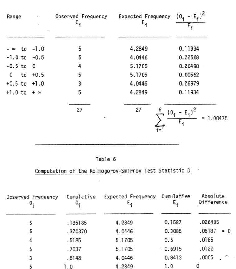
V.2.3. Chi-Square Goodness of Fit Test

In making this test one determines how closely the observed (sample) fre-quency distribution fits the normal probability distribution by comparing the

observed frequencies to the expected frequencies. The observed frequencies (calculated from the standardized residuals) are given in the second column of Table 5. The expected frequencies from the normal distribution are given in the third column. The remainder of the table is used to compute the value of the chi-square. The further the expected values from the observed values (the larger the 2 value is), the poorer the fit of the hypothesized

2

Figure C

Normal Probability Plot of Residuals

+2.0 +1.5 +1.0 +0.5 0 -0.5 -1.0 -1.5 -2.0 -. 075 -. 05 -. 025 0 +-025 +-05 Value of Residual + -0T5 +

,fi

Expected Normal Value -. 1

Table 5 Computation of Chi-Square Observed Frequency 0 Expected Frequency E i - 0 to -1.0 -1.0 to -0.5 -0.5 to 0 0 to +0.5 +0.5 to +1.0 +1.0 to + co 27 6 i =1 (0. - E 2 E 1 = 1.00475 Table 6

Computation of the Kolmogorov-Smirnov Test Statistic D

Observed Frequency

0

_i

Cumulative0 5 .185185 5 .370370 4 .5185 5 .7037 3 .8148 5 1.0. Expected Frequency E 4.2849 4.0446 5.1705 5.1705 4.0446 4.2849 Cumulative E 0.1587 0.3085 0.5 - 0.6915 0.8413 Absolute Difference .026485 .06187 = D .0185 .0122 .0005 1.0 0

Range _{(Oi - Ei) 2}

E. 4.2849 4.0446 5.1705 5.1705 4.0446 4.2849 0.11934 0.22568 0.26498 0.00562 0.26979 0.11934

2

significant even at the 0.05 probability level

(2

= 1.07), and it can be concluded that the hypothesized normal distribution fits the data satifac-torily.

V.2.4 Kolmogorov-Smirnov Test

Where the chi-square test requires a reasonably large sample, the Kolmogorov-Smirnov test can be used for smaller samples. The test uses a statistic called D, which is computed as follows:

Step 1 - Compute the cumulative observed relative frequencies. Step 2 - Compute the cumulative expected relative frequencies. Step 3 - Compute the absolute difference of both frequencies. Step 4 - The value of D is the maximum difference:

t t

D

max

.

(O/n) -

(Es/n)

t i=0 i=0

Step 5 - Compare D to critical values from the Kolmogorov-Smirnov tables.

The larger the value of D, the less likely the hypothesized normal distri-bution is suitable. Tables of the statistic D exist which give the critical

values for various probabilities and sample sizes [Miller, 1956]. For this case the critical value of D at a significance level of 0.10 and n=5

is 0.44698. Since the calculated value of D (0.06187) is less than the critical value, it is not significant and we again accept that our error

V.3 Test for Autocorrelation

The third assumption in the least-squares model Y = X + E represented by Equation (V.1) was that the error terms are uncorrelated random vari-ables. This assumption of independence is equivalent to assuming zero covariance between any pair of disturbances. A violation, referred to as autocorrelation, occurs if any important underlying cause of the error has a continuing effect over several observations. It is likely to exist if the error term is influenced by some excluded variable which has a strong cyclical pattern throughout the observations. If omitted variables are serially correlated, and if their movements do not cancel out each other, there will be a systematic influence on the disturbance term.

Besides the omission of variables, autocorrelation can exist because of an incorrect functional form of the model, the possibility of observation errors in the data, the estimation of missing data by averaging or extrapo-lating, and the lagged effect of changes distributed over a number of time periods [Huang, 1970].

The major impact of the presence of autocorrelation is its role in causing unreliable estimation of the calculated error measures. Goodness-of-fit statistics, such as the coefficient of multiple determination R , will have more significant values than may be warranted. In addition, the sample- variances of individual regression coefficients, such as price elasticity of demand, will be seriously underestimated, thereby causing the t-tests to produce wrong conclusions. Finally, the presence of sig-nificant autocorrelation will produce inefficient estimators [Elliott, 1973].

V.3.1 The Durbin-Watson Statistic

the Durbin-Watson statistic [Durbin-Watson, 1950-511. This statistic, d, is defined as follows: n 2 E (e. - e.1) d ==2 n 2 E e. i=1 I

where e. is the calculated error term resultig from the estimated regression equation. A positively autocorrelated error term will result in a dispro-portionately small value of the d statistic since the positive and nega-tive e. values tend to cancel out in the computation of the squared suc-cessive differences. A negative autocorrelated error term, however, will produce large values of d as the systematic sign changes cause successive terms to add-together. If no autocorrelation is present,d will have an expected value of approximately two. Two critical values of the d statistic, d and du, obtained from Durbin-Watson tables, are involved in applying the test. The critical values d and d describe the boundaries between the acceptance and rejection region for positive autocorrelation; and, the critical values 4-d and 4-du define the boundaries for negative auto-correlation. Forany remaining region the test is inconclusive. The posi-tive and negaposi-tive serial correlation regions, applicable for a 5 percent level of significance and the problem presented here, are shown in Figure D [Elliott, 1973].

Figure D

Acceptance and Rejection Regions

of the Durbin-Watson Statistic

Probability

of d 4- Reject (Positive Serial Correlation) Accept

(No Serial Correlation),

a

₁

a

_u 1.16 1.65 +-Reject (Negative Serial Correlation) 4-d 4-dl 2.35 2.84

Since the Durbin-Watson statistic for the model given by Equation (V.1) is equal to 0.77 it can be concluded that the residuals are positively

autocorrel ated.

V.4 Test for Multicollinearity

The fourth assumption built into the econometric model of Y = XS + E is that matrix X is of full rank. If this condition is violated, then the

determinant

IX'XI

is equal to zero, and the ordinary least-squares estimate b = (X'X)~l X'_{Y cannot be determined. In most air travel demand models} the problem is not as extreme as the case of

IX'XI

= 0. However, when the columns of X are fairly collinear such that

IX'XI

is near zero, then the variance of b, which is equal to a 2(X'X)~ , can increase significantly. This problem is known as multicollinearity. The existence of

multicol-linearity results in inaccurate estimation of the parameters S because of the large sample variances of the coefficient estimators, uncertain specification of the model with respect to the inclusion of variabl-es, and extreme difficulty in interpretation of the estimated parameters b.

The effects of multicollinearity on the specification of the air travel demand model are serious. For instance, it is a common practice among.demand analysts to drop those explanatory variables out of the model for which the t-statistic is below the critical level for a given sample size and level of significance. This is not a valid procedure since if multicollinearity is present, the variances of the regression coefficients under consideration will be substantially increased, and result in lower values of the t-statistic. Thus, this procedure can result in the rejection from the demand model of those explanatory variables which in theory do explain the variation in the dependent variable Y.

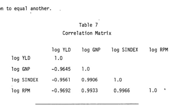
V.4.1 Correlation Matrix

In air travel demand models the problem is not so much in detecting the existence of multicollinearity but in determining its severity. The seriousness of multicollinearity can usually be examined in the correlation coefficients of the explanatory variables. How high can the correlation

coefficient reach before it is declared intolerable? This is a difficult question to answer, since it varies from case to case, and among different analysts. It is sometimes recommended, however, that multicollinearity can be tolerated if the correlation coefficient between any two explanatory variables is less than the square root of the coefficient of multiple

determination [Huang, 1970]. An examination of the correlation matrix for the sample case (Table 7) clearly indicates significant correlation between the explanatory variables. The analyst should be cautious, however, in examining multicollinearity by using the simple correlation coefficients since such a rule is useful only- for pairwise considerations; for instance, even if two columns may not be highly collinear, the determinant of (X'X) will be zero if several columns of X can be combined in a linear combina-tion to equal another.

Table 7 Correlation Matrix

log YLD log GNP log SINDEX log RPM log YLD 1.0

log GNP -0.9645 1.0

log SINDEX -0.9561 0.9906 1.0

log RPM -0.9692 0.9933 0.9966 1.0

V.4.2 Eigenvalues

The degree of multicollinearity can also be reflected in the eigen-values of the correlation matrix. To demonstrate this it is necessary to represent the regression model in matrix notation. Let Y = X + 6 be the regression model where it is assumed that X is (n x p) and of rank p,

5 is (p x 1) and unknown, E[s] = 0, and E[sE'] = 12'.Let5 be the least squares estimate of 6, so that:

= (X'X)~1 X'Y (V.6)

Let X'X be represented in the form of a correlation matrix. If X'X is a unit matrix,

X'X = =I.

n

then the correlations among the X are zero, multicollinearity does not exist, and the variables are said to be orthogonal. However, if X'X is not nearly a unit matrix, multicollinearity does exist, and the least

squares estimates, S , are sensitive to errors. To demonstrate the effects of this condition Hoerl and Kennard [1970] propose looking at the distance between the estimate S and its true value S. If L is the distance from

6 to 6, then the squared distance is:

L2 = (S -

s)'(6

- 6) *(V.7)

2

Analogous to the fact that E[cc'] =a I , the expected value of the squared distance L2 can be represented as:

E[L2] = Trace (X'X)~1 (V.8)

If _{the eigenvalues of X'X are denoted by XMAX = X1 >X2 ' Xp}

then the average value of the squared distance from S to 6 is given by:

E2 _2' 2

EEL 2] = aY P ( >. >a2 /X(V)

1 1

This relationship indicates that as X decreases, E[L 2 increases. Thus, if X'X results in one or more small eigenvalues, the distance from S to S will tend to be large, and large absolute coefficients are one of the

effects or errors of nonorthogonal data.

The X'X matrix in correlation form was given in Table 7. The result-ing eigenvalues of X'X are:

AYLD = 2.933 XGNP = 0.059 XSINDEX = 0.008

Note the smallness of XYLD and XSINDEX, which reflects the multicollinearity problem. The sum of the reciprocals of the eigenvalues is

I(1/X ) = 1/2.933 + 1/0.059 + 1/0.008 = 142.29

Thus, equation (V.9) shows that the expected squared distance between

A 2

the coefficient estimate S and S is 142.29 a , which is much greater than what it would be for an orthogonal system (3 a2

V.4.3 Farrar and Glauber Test to Identify Variables Involved in Multicollinearity

To identify which individual variables are most affected by collinear-ity, an F-distributed statistic proposed by Farrar and Glauber [1967], tests the null hypothesis (H : X. is not affected) against the alternative

(H X is affected).

Recalling that (X'X) is the matrix of simple correlation coefficients for X, as interdependence among the explanatory variables grows, the cor-relation matrix (X'X) approaches singularity, and the determinant

IX'XI

approaches zero. Conversely, |X'XI close to one implies a nearly orthog-onal independent variable set. In the limit, perfect linear dependence among the variables causes the inverse matrix (X'X)~1 to explode, and the diagonal elements of (X'X)~ become infinite. Using this principle, Farrar and Glauber define their test statistic as:

*j (n-p)

F p= r - 1) (V.10)

(n-p, p-1)(p1

where r denotes the jth diagonal element of (X'X)~1, the inverse matrix of simple correlation coefficients. The null hypothesis (H0 X is not affected) is rejected if the calculated F-distributed statistic exceeds the critical F(a; n-p, p-1). The results for the model of Equation (V.1) are given in Table 8. The calculated F-statistics,

Fln YLD = 110.02 Fl GNP = 497.23 , and Fln SINDEX = 402.37 ,

are all much greater than the critical F(.05, 27-4, 4-1) = 8.64. Thus, the null hypothesis can be rejected and the alternate, that all variables are significantly affected by multicollinearity, can be accepted.

Table 8

Farrar and Glauber Test for Multicollinearity Simple Correlation Matrix

in YLD in GNP in SINDEX

1.0 -0.964 -0.956

(X'X) = -0.964 1.0 0.991

-0.956 0.991 1.0

Determinant = 0.0013

Inverse Correlation Matrix

in YLD in GNP in SINDEX r* n YLD r in GNP 14.344 = 13.329

r*

In

SINDEX

0

.

511

13.329 0.511 65.828 -52.466 -52.466 53.461 = (14.344 - 1) (27-4)_4-17 = (14.344)(7.67) = 110.02 = (65.828 - 1)(7.67) = 497.23 = (53.461 - 1)(7.67) = 402.37 (X'X)~ -Fin YLD Fin GNP FlIn SINDEX

V.5 Summary Evaluation of the Ordinary Least-Squares Model

The method of least-squares produces estimators which are unbiased, efficient and consistent if the assumptions regarding homoscedasticity, normality, no autocorrelation, and no multicollinearity can be made with respect to the disturbance term and the other explanatory variables in the model. This section tested each of these assumptions on the ordinary least-squares model of Equation (V.1). The conclusions are:

. the sample data is homoscedastic,

. the distribution of error terms is normal

. the residuals are positively autocorrelated,

. severe multicollinearity exists among all explanatory variables. Thus, the least-squared model failed on the autocorrelation and

multicollinearity tests.

The autocorrelation problem may adversely affect the property of the least-squares technique to produce efficient (minimum-variance) estimates. This means that the resulting computed least squares plane cannot be relied on, and the goodness-of-fit statistics, such as the R2 and the t-test, will have more significant values than may be warranted. The existence of severe multicollinearity compounds these problems. When the columns of X are fairly collinear such that the determinant -IX'XI is near zero, then the variance of the estimators b, which is equal to a2(X'X)~l can increase significantly. This results in inaccurate estimation of parameters B

because of the large sample variances of the coefficient estimators,

un-certain specification of the model with respect to the inclusion of variables, and extreme difficultly in interpretation of the estimated parameters b.

45

In the sections that follow, the autocorrelation problem will be corrected by the method of generalized least-squares, and the problem of severe multi-collinearity will be dealt with using a relatively new (1970) technique called

VI. Correction for Autocorrelation - Generalized Least Squares

The problems associated withthe presence of autocorrelation (inflated R2 unreliable estimates of the coefficients, inefficient estimators) are already well documented [Taneja, 1976].Standard procedures, such as the Cochrane-Orcutt

[1949] iterative process, are available for correcting autocorrelation, but the procedure, which usually requires a first or second difference transfor-mation of the variables:

Y -

Y = (X- p X) + (e- p ) (VI.)

where p is es-tImat-ed from e P-e

and e is the vector e lagged one period,

restricts the forecasting interval to one period - which is very limiting for long term forecasting. Another method, known as generalized least squares, corrects for autocorrelation and is not as restrictive as the Cochrane-Orcutt process.

The classical ordinary least squares (OLS) linear estimation procedure is characterized by a number of assumptions concerning the error term in the regression model. Specifically, the disturbance term c in

Y = X + e (VI.2)

is supposed to satisfy the following requirement:

E[EE']

=

a

2

p

₌

[2

₁

_(VI.3)

the variances of the disturbance terms are constant and the covariances are zero, COV(E s ) = 0, for i / j. If the disturbance terms at different obser-vations are dependent on each other, then the dependency is reflected in the correlation of error terms with themselves (i.e. in the covariance terms) in preceding or subsequent observations. This autocorrelation of disturbance terms violates the assumption given by Equation (VI.3).

If this assumption (VI.3) is not made, but all the other assumptions of the OLS model are retained,the result is a generalized least squares (GLS) regression model. The GLS model is:

Y = Xl + E , (VI.4)

for which the variances of the disturbance terms are still constant but the covariances are no longer zero, COV( £ E) / 0, for i / j. Consequently,

the variance-covariance matrix of disturbances for the first-order autore-gressive process

Et P £ t-l + U (VI.5)

(where u is distributed as N(0, a'2_{I) and |pJ < 1) is given by [Kmenta, 1971]:}

E[. ' = a 2 (VI.6) 1 t-12 11 p2.. Qt S 2 2 . t-3 't-l't-72 t-'3-0-- (VI.7) P P P i

In OLS the estimate of 6 is given by:

=

(X'X)~

X'Y

.

(VI.8)

In GLS the estimate of F is given by:

F = (X'~1X)1 (X'~Y). (VI.9)

The preceding discussion has been carried out on the assumption that 2, the variance-covariance matrix of the disturbances, is known. In many cases Q is not known. But if the disturbances follow a first-order autoregressive scheme,

Et "t-1 E + U (VI.10)

then S1 involves only two unknown parameters, a2 _{and p, which can be} readily estimated.

A version of the generalized least squares regression technique is programmed into the TROLL computer software system developed at the National Bureau of Economic Research. TROLL automatically performs an iterative search for the best value of the p parameter. The results of this search are:

log RPM = 2.133 - 0.794 log YLD + 1.467 log GNP + 0.652 log SINDEX

(1.291) (-3.646) (6.121) (4.7a1)

R2 = 0.9757 (VI.ll)

Standard Error of Estimate = 0.0349

n = 27

Durbin-Watson = 1.89 p = 0.8796