Trade costs and the Home Market Effect

HAL Id: hal-00497693

https://hal.archives-ouvertes.fr/hal-00497693

Submitted on 25 Jul 2011

HAL is a multi-disciplinary open access

archive for the deposit and dissemination of sci-entific research documents, whether they are pub-lished or not. The documents may come from

L’archive ouverte pluridisciplinaire HAL, est destinée au dépôt et à la diffusion de documents scientifiques de niveau recherche, publiés ou non, émanant des établissements d’enseignement et de

Trade costs and the Home Market Effect

Matthieu Crozet, Federico Trionfetti

To cite this version:

Matthieu Crozet, Federico Trionfetti. Trade costs and the Home Market Effect. Journal of Interna-tional Economics, Elsevier, 2008, 76 (2), pp.309-321. �10.1016/j.jinteco.2008.07.006�. �hal-00497693�

Trade Costs and the Home Market Effect.

∗

Matthieu Crozet

Federico Trionfetti

October, 2007

Abstract

Most of the theoretical and empirical studies on the Home Market Ef-fect (HME) assume the existence of an “outside good” that absorbs all trade imbalances and equalizes wages. We study the consequences on the HME of removing this assumption. The HME is attenuated and, more interestingly, it becomes non-linear. The non-linearity implies that the HME is more impor-tant for very large and very small countries than for medium size countries. The empirical investigation conducted on a database comprising 25 indus-tries, 25 counindus-tries, and 7 years confirms the presence of the HME and of its non-linear shape.

Keywords: International Trade, Test of Trade Theories, Economic

Geog-raphy.

JEL Codes: F1, R12.

∗_{We are grateful to Thierry Mayer and Soledad Zignago for having provided us with data.}

We thank Tommaso Mancini-Griffoli for helpful advice and Rosen Marinov for excellent research assistance. We are grateful to anonymous referees for their comments, which proved very useful in clarifying and improving the paper. Authors are grateful, respectively, to the ACI - Dynamiques

de concentration des activit´es ´economiques dans l’espace mondial and to the Swiss National Funds

for financial support.

†_{University of Reims; CEPII; and Centre d’Economie de la Sorbonne. crozet@univ-paris1.fr.}

Postal address: CEPII, 9 rue Georges Pitard, 75015 Paris, France.

1

INTRODUCTION

Models characterized by the presence of increasing returns to scale, monopolistic competition, and trade costs typically give rise to what has become known as the Home Market Effect after Krugman (1980) and Helpmand and Krugman (1985). The Home Market Effect (HME) is defined as a more-than-proportional relationship between a country’s share of world production of a good and its share of world demand for the same good. Thus, a country whose share of world demand for a good is larger than average will have - ceteris paribus - a more than proportionally larger-than-average share of world production of that good.1 _{The HME is so closely}

associated to the presence of increasing returns to scale (IRS) and monopolistic competition (MC) that it has been used as a discriminating criterion to testing trade theory in a novel approach pioneered by Davis and Weinstein (1999, 2003). Since then, as it will be discussed below, further theoretical and empirical research has explored the robustness of the HME and has searched for additional discriminating criteria.

One pervasive assumption in the literature to date is that of the presence of a good freely traded and produced under constant returns to scale (CRS) and per-fect competition (PC). This good is often referred to as the “outside good”. The presence of the outside good serves two purposes. First, it guarantees factor price equalization, thereby improving grandly the mathematical tractability of models. Second, it offsets all trade imbalances in the IRS-MC good, thereby permitting in-ternational specialization. A different way of seeing the second point is that the outside good accommodates all changes in labor demand caused by the expansion or contraction of the IRS-MC sector, thereby allowing for the reaction of production to demand in the latter sector to be more than proportional. The assumption of the existence of a freely traded CRS-PC good is as much convenient as it is at odds with reality. As noted by Head and Mayer (2004, p. 2634) when discussing this issue in their comprehensive account of the literature:“. . . the CRS sector probably does not have zero trade costs or the ability to absorb all trade imbalances.” The pervasive use of the outside good assumption and its inconsistency with reality raise

1_{An alternative definition of the HME often used in the literature is that a country whose share}

of demand for a good is larger than average will be a net exporter of that good. In this paper we will always refer to the HME as the more than proportional relationship between the share of production and the share of demand.

the question of what are the consequences of its removal on the HME. The present paper investigates this question.

We eliminate the outside good from the main model used in the empirical lit-erature on the HME. This model, in two different variants, has been used in Davis and Weinstein (1999, 2003) and in Head and Ries (2001). We find that, in general, the HME survives when the outside good is absent but its average magnitude is attenuated. More interestingly, both variants of the model predict a non-linear re-lationship between the production share and the demand share. The non-linearity is characterized by a tenuous HME (or absence thereof) when countries’ demand shares are not too different from the world average. The HME becomes stronger when countries’ demand share become more dissimilar. We put this result to em-pirical verification on a data set containing 25 countries, 25 industries and 7 years. The non-linearity predicted by both models is strongly present in the data. One interesting consequence of the non-linearity is that the HME is more important for countries whose magnitude of demand shares is very different from the average than for countries whose demand shares are closer to the average. Performing a test of structural change with unknown breakpoints shows indeed that the HME matters only for the largest and smallest demand share, accounting for about one fifth of the observations in the sample. For the remaining observations, the HME is of negligible importance or totally absent.

As for the CRS-PC sectors, the model shows that the less-than-proportional re-lationship between share of production and share of demand survives the absence of an outside good. This result, combined with the more than proportional relationship between share of production and share of demand in the IRS-MC industry, confirms the theoretical validity of the HME as a discriminating criterion to test trade the-ories even in the absence of an outside good. The empirical investigation in this paper finds little evidence of sectors exhibiting a less than proportional relationship. The remainder of the paper is as follows. Section 2 discusses the related litera-ture, section 3 presents the model and the theoretical results, section 4 presents the empirical results, and section 5 concludes. The appendix discusses the numerical method, derives analytical results, and presents some robustness checks.

2

RELATIONSHIP TO THE LITERATURE

In the model structures of Krugman (1980) and Helpman and Krugman (1985) the HME is a feature of the IRS-MC sectors and not of the CRS-PC sectors. This distinction has been used to test the empirical merits of competing trade theories. Davis and Weinstein find stronger evidence of the HME at the regional level (Davis and Weinstein 1999) than at the international level (Davis and Weinstein 2003). Head and Ries (2001) consider a model where, in addition to the outside good and the IRS-MC good, there is also a CRS-PC good characterized by National Product Differentiation `a la Armington (1969). In such model, the IRS-MC good exhibits the HME while the Armington good does not. Using data for U.S. and Canadian manufacturing they find evidence in support of both the IRS-MC and the Armington market structure depending on wether within or between variations are considered. Both Davis and Weinstein (1999 and 2003) and Head and Ries (2001) assume the existence of an outside good. The first investigation on the consequences of removing the outside good is found in Davis (1998). He eliminates the outside good from the model in Helpman and Krugman (1985, Ch. 10) by introducing trade costs in the CRS-PC good. His theoretical paper has shown that in the absence of an outside good the HME may disappear. The HME disappears if and only if trade costs in the CRS-PC good are sufficiently high to impede international trade in this good. Does the HME survive and what shape does it take when trade costs in the CRS-PC good are not high enough to impede trade in this good? This question, which we address both theoretically and empirically in part of this paper, remains unanswered in Davis (1998).

Other papers have addressed the issue of trade costs and international special-ization without, however, focusing on the shape of the HME or on the validity of the HME as discriminating criteria. In a theoretical paper, Amiti (1998) studies, among other things, how the pattern of specialization and trade varies with country size when industries have different trade costs. Laussel and Paul (2007), use a two-sector model where the elasticity of substitution differs between industries. They find that, if countries are close in size, a fall in transport costs from a prohibitive level to zero is associated with a reversal in the pattern of trade at some interme-diate level of trade costs. If the two countries are instead very different in size the larger country is always a net exporter of the less differentiated good. Hanson and

Xiang (2004) theoretically and empirically investigate the pattern of specialization and trade in a model where a continuum of IRS-MC goods differ in terms of elas-ticities of substitution and trade costs. Holmes and Stevens (2005) focus on how the pattern of trade varies across industries that differ in technology when there are equal trade costs in all sectors. While these papers address issues related to the one in the present study, their focus is different from ours.2 _{The robustness of the HME}

is the subject of investigation also in Head, Mayer and Ries (2002), yet with focus on the role of market structure rather than on the role of the outside good. They study the robustness of the HME to three different modeling assumptions concern-ing the market structure: Cournot oligopoly and homogenous good, monopolistic competition with linear demand, and Cournot oligopoly with national product dif-ferentiation. They find that the first two types of market structure yield a linear relationship between the share of production and the share of demand. The third market structure, instead, give results that depend on the elasticity of substitution between domestic and foreign goods.3

3

THE MODEL

In this section we study the consequences that the absence of an outside good has on the HME using a theoretical model. The model is characterized by the presence of two goods: a good produced under IRS-MC, named M; and a good produced under CRS-PC, named A. The latter is differentiated by country of production `a la Arm-ington (1969). For notational convenience we shall refer to this good as the CRS-PC-A good. Individuals have the following two-tier utility function: U = Mγ_A1−γ_,

where γ ∈ (0, 1) is the expenditure share on good M . Good M is a CES aggre-gate of all varieties of M produced in the world, M = ³R_κ∈Ω(cM k)

σM −1 σM dk

´ σM σM −1

,

2_{Other papers have studied different manifestations of the HME while keeping the assumption}

of the existence of an outside good whenever appropriate. Such papers include Weder (1995), Lundb¨ack and Torstensson (1999), Feenstra, Markusen and Rose (2001), Trionfetti (2001), Weder (2003), Yu (2005), and Br¨ulhart and Trionfetti (2005).

3_{In the third market structure, for intermediate and high values of the elasticity of substitution}

there is no HME and the relationship between production and demand may be non-linear. The model based on this market structure, however, is not suitable to address the question of the robustness of the HME to the absence of the outside good since it does not predict the HME for any value of parameters. Further, its structure makes it hardly comparable to the models most widely used for theoretical and empirical purposes.

where Ω is the set of of all the varieties of M produced in the world, cMk is

con-sumption of variety k, and σM is the elasticity of substitution between any two

varieties. Good A is a CES aggregate of the domestic and foreign variety of A,

A =

³ (cA1)

σA−1

σA _{+ (cA2)}σA−1σA

´ σA σA−1

, where cAi is consumption of country i’s variety

of good A and σA is the elasticity of substitution between the domestic and the

for-eign variety of A. Good A is produced under constant returns to scale and perfect competition, there is an infinity of domestic producers and an infinity of foreign pro-ducers. Consumers perceive the domestically produced A as different from foreign

A but they perceive as identical the output of two producers in the same country.

There is, therefore, product differentiation by country of production. That is, con-sumers care about the “made in” label. In models of trade in the spirit of Helpman and Krugman (1985) the CRS-PC good is assumed to be perfectly homogenous internationally; thus, domestic and foreign A are perfect substitute. Assuming per-fect substitutability and absence of the outside good gives the knife-edge result that we derive in Section 3.2. We do not limit our investigation to the case of perfect substitutability. We allow for a more general case where the domestic and foreign CRS-PC goods are not perfect substitute. This slight generalization will allow us to verify the robustness of the knife-edge results generated by the assumption of perfect substitutability.

From utility maximization and aggregation over individuals in the same country we have the following demand functions (the first subscript indicates the country where the good is produced, the second subscript indicates the country where the good is sold): mii = p−σM iiMPM iσM−1γYi, mij = p−σM ijMPM jσM−1γYj, aii= pAii−σAPAiσA−1(1 − γ) Yi, aij = p−σAijAPAjσA−1(1 − γ) Yj; where mii and mij represent, respectively, domestic and

foreign residents’ demand for any of the domestic varieties of M; similarly, aii and aij represent, respectively, domestic and foreign residents’ demand for the

domes-tic production of A. Demand functions depend on prices and income: pM ii and pM ij represent, respectively, the price in country i and j of a variety produced in i; pAii and pAij represent, respectively, the price in i and j of good A produced in i; PM i= ³R κ∈Ωi(piik) 1−σM _{dk +} R κ∈Ωj(pjik) 1−σM _dk ´ 1 1−σM

is the CES price index of M relevant for consumers in country i and Ωi is the set of varieties produced in

country i; PAi =

¡

p1−σA

Aii + p1−σAjiA

¢ 1

1−σA _{is the CES price index of A relevant for}

wage and labor endowment in country i.

We assume iceberg transport costs in both sectors. Thus, τM ∈ (0, 1) and

τA ∈ (0, 1) represent for M and A, respectively, the fraction of one unit of good

sent that arrives at destination. It is convenient to define: φM ≡ τMσM−1 ∈ (0, 1),

and φA ≡ τ_AσA−1 ∈ (0, 1). Trade freeness in anyone sector increases when the value

of the corresponding phi increases.

Production technology of any variety of M exhibits increasing returns to scale. The labor requirement per q units of output is: LM = F + aMq. The production

technology of A exhibits constant returns to scale. To save notation we assume that one unit of labor input produces one unit of output of A. Profit maximization gives the following optimal prices:

pAii = wi, pM ii= σM σM − 1 aMwi, i = 1, 2. (1) pAij = 1 τA pAii, pM ij = 1 τM pii, i 6= j, i, j = 1, 2. (2)

The zero profit condition gives the firm’s optimal size, which turns out to be the same in both countries and for all firms:

qi = F

aM

(σM − 1), i = 1, 2. (3)

Using demand functions and Walras’ law the equilibrium conditions in the goods market are: pM 11q1 = p 1−σM M 11 γw1L1 p1−σM M 11 n1+ φMp 1−σM M 22 n2 + φMp 1−σM M 11 γw2L2 φMp1−σ_{M 11}Mn1+ p1−σ_{M 22}Mn2 (4) pM 22q2 = φMp1−σM 22Mγw1L1 p1−σM M 11 n1+ φMp1−σM 22Mn2 + p 1−σM M 22 γw2L2 φMp1−σM 11Mn1+ p1−σM 22Mn2 (5) pA11A1 = p1−σA A11 (1 − γ) w1L1 p1−σA A11 + φAp1−σA22A + φAp 1−σA A11 (1 − γ) w2L2 φAp1−σA11A + p1−σA22A (6) Equilibrium conditions in labor markets are:

L1 = A1+ n1(F + aMq1) (7)

L2 = A2+ n2(F + aMq2) (8)

The fifteen equations (1)-(8) determine the fifteen endogenous variables of the model. These are the eight prices: pA11, pA12j, pA22, pA21, pM 11, pM 12, pM 22, pM 21;

firm’s optimal size in each country: q1, q2; the number of varieties of M produced in

each country: n1, n2; the production of A in each country, A1, A2, and the relative

wage ω ≡ w1

w2. The exogenous variables include all parameters and - importantly

for our purposes - the size of countries measured by labor endowments, represented by L1 and L2. It is convenient to make use of the following definitions of share

variables: SN i ≡ _n1n_+ni ₂, represents country i’s share of world production of M; SAi ≡ _A1A_+Ai ₂, represents country i’s share of world production of A; SLi ≡ _L1L_+Li ₂,

represents country i’s share of world endowment of labor; and SIi ≡ _w1Lw_1+wiLi_2L2

represents country i’s share of world expenditure (on any one good).

Models in the vein of Helpman and Krugman (1985, Ch. 10) predict a more than proportional relationship between a country’s share of production and its share of labor endowment, this is the HME, that is: dSN i

dSLi > 1. They also predict a

less than proportional relationship between a country’s share of production and its share of labor endowment for CRS-PC sectors, that is: dSAi

dSLi ∈ [0, 1). These

predictions obtain in the presence of an outside good. The contrast between the more than proportional relationship in IRS-MC sectors and the less than proportional relationship in the CRS-PC sectors constitutes a discriminating criterion usable for testing trade theories. We want to verify whether the HME and the discriminating criterion are robust to the absence of the outside good. To this purpose we compute the derivatives dSN i

dSLi and

dSAi

dSLi in our model. We do so for the two major cases used

in the empirical literature. First, we will assume that σA = σM. This assumption,

abstracting from the absence of an outside good in our model, brings us to the framework used in Head and Ries (2001). Second, we will assume that σA 6= σM

and that σA = ∞. This assumption brings us exactly in the model developed in

Davis (1998).

The functional relationships we study always relate one of country i’s share variables to country i’s share of labor endowment. Henceforth, we drop the subscript

i since confusion does not arise.

3.1

Finite Elasticities (1 < σ

= σ

< ∞)

We want to find out the shape of the functional relationship between the share of production and the share of labor endowment in the incomplete specialization set. This functional relationship cannot be obtained explicitly given the kind of non linearity of the system composed by equations (1)-(8). We therefore obtain the results by numerical exploration of the model. The numerical method is explained in section 6.1 of the appendix.

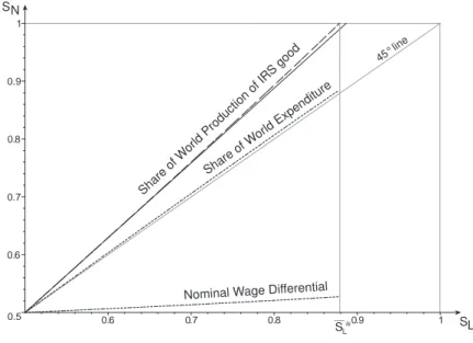
Figure 1 illustrates the results. The figure shows the numerical solution for the following parameter values: σA = σM ≡ σ = 7, γ = 3, τA = 0.6, τM = 0.8.

Naturally, the figure is representative of the pattern found on all the numerical solutions. There are five functions plotted in the figure. To facilitate the visual inspection we have exploited the symmetry of all functions around the symmetric equilibrium and “zoomed” into the zone delimited by the sets [1/2, 1] and [1/2, 1] on the abscissa and ordinates. All functions are plotted within the incomplete specialization set (SLis and SL

is

). Because of the “zooming”, Figure 1 shows only the upper half of the incomplete specialization set. Only the upper bound of it,

SL is

, is marked in the figure. We address the functions by descending order of slope. The first function (represented by a dashed curve) shows the function SN(SL). The

second function (represented by a continuous straight line) is a linear function whose slope at SL = 1/2 is the same as the slope of the dashed curve. Visual inspection,

taking account of the above-mentioned symmetry, shows that SN(SL) exhibits the

HME since its slope is larger than 1 everywhere within the incomplete specialization set. Further, and more interestingly, the function SN(SL) is concave to the left of

1/2 (not shown in the figure), it has an inflexion at SL= 1/2 and it is convex to the

right of 1/2. The non-linearity is tenuous, however, as shown by the fact that the dashed curve and the continuous straight line are almost indistinguishable at naked eye. These result, which are found in all numerical solutions, can be summarized as follows:

Result 1. When elasticities are finite, the absence of the outside good makes the

HME non-linear with shape concave-inflexion-convex; the non-linearity is tenuous, however. We refer to this shape as the “smoothly non-linear HME”.

Figure 1: Smoothly non-linear HME 0.5 0.6 0.7 0.8 0.9 1 0.6 0.7 0.8 0.9 1 Share o f World Expen diture Share of W orld Produc tion of IRS g ood SN SL 45°l ine

Nominal Wage Differential

S_Lis

So far we have focused on the relationship between the real variables SN and (SL).

This is indeed at the center of our interest since we want to study the relationship between a country’s relative size (measured by endowment) and its international specialization (measured by relative size of physical output in each industry). How-ever, the way the HME is usually understood is that a shock to a country’s share of factor endowment generates a shock of the same sign to its share of expenditure which, in turn, affects the share of physical output. This is indeed what happens in our model and it is shown by the third function (represented by the dotted curve) which shows the variable SI as function of SL: an increase in the country’s physical

endowment of labor causes an increase in its share of world expenditure (on any good).4

Before passing to the next section we report that the shape of the function

4_{A brief discussion on wages is in order. The numerical exploration has shown that the wage}

ratio ω may be increasing or decreasing in SL. However, SI is always increasing in SL. The

ambiguity on the sign of the slope of ω is the consequence of two opposite forces: the presence of the M industry tends to give a positive slope (the largest country would have the largest wage) but the presence of the A industry pushes wages in the opposite direction. Overall, even when

ω is decreasing in SL, its decline is not enough to outweigh the effect that an increase in SL has

on SI. The lowest dotted line in Figure 1 represent the nominal wage differential plotted for the

parameter values recalled above and shifted up by 1/2 so that it can be plotted in the same range as the other functions (the function plotted is w1 − w2 + 1/2).

SA(SL), not shown in the figure, mirrors that of SN(SL) around the 45-degree line

in the entire incomplete specialization set. The function SA(SL) has shape

“convex-inflexion-concave” and its slope is always smaller than one.

3.2

Perfect substitutability in the CRS-PC good (σ

= ∞)

When good A is perfectly homogenous internationally the resulting model is exactly as in Davis (1998). The major finding of Davis’ paper is that the HME disappears when trade costs in A are sufficiently high to eliminate trade in that good. Our focus is to study the shape of SN(SL) when trade costs are not sufficiently high to

eliminate trade in A. This aspect remains unexplored in Davis’s paper. In section 6.2. of the appendix we obtain explicit solutions for the model. The logic of the results is simple, however. When trade costs in A as sufficiently large, industry M cannot expand more than proportionally because industry A cannot release labor. Industry A cannot release labor because, if there is no trade in A, domestic produc-tion of A must satisfy domestic demand. In the absence of trade in A, a country’s share of production of A must be proportional to its share of demand. Consequently, the country’s share of production of M must also be proportional to its share of de-mand. When trade in A occurs there is HME in M. The reason is that industry A no longer needs to satisfy domestic demand (good A can be imported) and therefore it can release labor to industry M, which can expand more than proportionally. The existence of the HME in this model, therefore, depends crucially on whether trade costs in A are high enough to eliminate trade in this good. The sufficient condition for the HME to exist is τA> τ

σM −1 σM

M .

Figure 2 shows the results. The dashed broken line represents the function

SN(SL) resulting from the explicit solution of the model (plotted for σM = 3, τM = 0.7, τA = 0.9). Again, because of the zooming we see only the upper half of

all functions and sets. The figure shows that the relationship between SN and SL

is perfectly proportional in the set ¡SL, SL

¢

. There is no HME in this set. Instead, there is HME for values of SL in

¡

SLis, SL

¢

- not shown in the figure - and in (SL, SLis). The relationship between SN and SL is more than proportional in these

sets. Further, the more than proportional bit of SN(SL) in

¡

SLis, SL

¢

is concave - not shown in the figure. Instead, the more than proportional bit of SN(SL) in

Figure 2: Piecewise non-linear HME 0.5 0.6 0.7 0.8 0.9 1 0.6 0.7 0.8 0.9 1

Nominal Wages Dif ferential 45°l ine Share of W orld Produc tion of I RS Good SN SL SL is S L (SL, SL is

) is convex.5 _{We can summarize the result as follows:}

Result 2. When σA= ∞ and when there is trade in A the HME is non-linear with shape “concave-linear-convex”. We refer to this shape as the “piecewise non-linear HME”.

The dotted broken line in Figure 2 shows the nominal wage differential shifted up by 1/2 so that it can be plotted in the same range as the other functions (the function plotted is w1−w2+1/2). The wage differential is an increasing function of SLin the

set (SL, SL). Instead, the wage differential is flat in (SLis, SL), and (SL, SLis). This

shape of the wage differential (which obtains for any value of parameter) implies that an increase in the share of labor endowment causes an increase in the share of expenditure. The function SI(SL) - not plotted in Figure 2 - is therefore increasing

in SL.

The shape of the function SA(SL), not shown in the figure, mirrors that of SN(SL) around the 45-degree line in the entire incomplete specialization set. The

function SA(SL) has shape ”convex-linear-concave” and its slope is always smaller

than one.

An increase of trade costs in A relative to M expands symmetrically the set ¡

SL, SL

¢

which then covers a larger sub-set of (0, 1). If trade costs in A are suf-ficiently high the set ¡SL, SL

¢

coincides with (0, 1) and the HME disappears com-pletely.

Before passing to the empirical part it is convenient to mention that the model presented above, like other models in the same spirit, predicts that higher elasticities of substitution and higher trade costs attenuate the Home Market Effect. Moreover, higher elasticities of substitution and higher trade costs make also the Home Market Effect more linear. These predictions are not at the heart of our investigation and, for reason of space, we do not provide a demonstration but we will refer to them in the empirical section below.

4

EMPIRICAL IMPLEMENTATION

The model examined in the previous section gives the following prediction: removing the outside good makes the HME non linear by either giving it the smooth shape (Figures 1) or the piecewise shape (Figure 2). The HME is weaker (if it exists at all) nearer the symmetric equilibrium than away from it. Therefore, its impact is bigger for countries whose demand shares are very different from the world average than for countries whose demand shares are near the world average.

These results can be verified empirically by analyzing the relationship between countries’ production shares and demand shares. In this section we estimate the effect of each demand deviation from the sample average on the corresponding pro-duction deviation for a large set of countries and industries.

4.1

Variables and data

The empirical investigation of the model requires reliable measures of demand and production deviations by countries and industries.

Let xikt denote the quantity of good k produced in country i at date t. The

supply deviation in country i for product k at time t is:

∆S,ikt= xikt P_R i=1xikt − 1 R,

where R is the number of countries. ∆S,ikt is positive if the production of good k in country i is greater than the mean value of the sample, and negative otherwise.

To be consistent with the theoretical model, we measure ∆S,ikt in terms of quantity

of production. We proxy the quantities by xikt = Xikt/pikt, where Xikt is the value

of production of good k in country i at date t and piktis the price of that production.

The demand deviation variable, ∆D,ikt, is defined similarly:

∆D,ikt =

Dikt/pikt

P_R

i=1(Dikt/pikt)

− 1

R.

The variable Dikt captures the demand potentially addressed to producers of

good k in country i. It is the value of demand emanating from all countries for good k produced in country i at date t. It is computed as the sum of sectoral expenditures in all locations weighted by accessibility to consumers.6 _Denoting

with Ejkt the expenditure on good k in country j and with Φijkta measure of trade

freeness, we have: Dikt =

P_R

j=1ΦijktEjkt.

An important issue for empirical investigation lies in the measurement of trade freeness represented by the parameter Φijkt. We use here the same estimate of trade

barriers as Head and Ries (2001). Starting from the theoretical demands expressed on foreign and domestic markets, and assuming symmetric bilateral trade freeness and free trade within countries, they obtain the following proxy for Φijkt:

ΦHR ijkt = r zijktzjikt ziiktzjjkt ,

where zijkt is the value of the trade flow of good k, from i to j at year t and ziikt is country i’s imports from itself. The index ΦHRijkt ranges from 0 to 1, with 1

denoting free trade.7

The measure of trade freeness proposed by Head and Ries (2001) has three main qualities. First, ΦHR

ijkt is time-dependent, so that it controls for the potential changes

in access to market due to trade liberalization processes. Second, ΦHR

ijktencompasses

all possible sources of bilateral trade barriers, besides trade frictions associated to geographical distances and other usual gravity inputs. Third, ΦHR

ijkt does not impose

6_{Davis and Weinstein (2003) call this variable the “Derived Demand”, and Head and Mayer}

(2006) refer to it as the “Nominal Market Potential”.

7_{Head and Mayer (2004) discuss further this index. Alternatively, Davis and Weinstein (2003)}

any strict assumption on bilateral trade relation and fits specifically to each country-pair. This is very important for the purpose of this paper; since we are looking for nonlinearity in the HME relation, we have to make sure that our measure of access to market does not introduce a bias that especially affects outlier trading countries. The empirical investigation of the model requires compatible data of production and demand at the sectoral level. Moreover, we need bilateral trade data for the corresponding products and countries in order to compute ΦHR

ijkt. We use the trade

and production database provided by CEPII. This database uses the source (BACI) and the source OECD-STAN to expand the trade and production database compiled by the World Bank.8 _{The CEPII’s trade and production database provides figures}

on sectoral production, prices, total exports and imports, and bilateral trade for a large set of industries (ISIC-Rev. 2) and countries, over 25 years (1976-2001). For each country and sector, intra-national trade is computed as the difference between country’s sectoral production and its aggregate sectoral exports to all other nations. Similarly, domestic expenditure is the sum of this non-exported production and the sectoral imports from the rest of the world. Missing values forced us to eliminate some countries and industries. The resulting data set reduced to a balanced 25 countries and 25 industries data set over the period 1990-1996.9

4.2

Pooled results: the shape of the HME

We begin by showing the empirical evidence on the pooled sample. These pooled tests give an informative outline of the patterns of the HME and allow some direct comparisons with previous research.

Figure 3 plots ∆S,ikt against ∆D,ikt for the 25 industries and the 25 countries

for the year 1996. As expected, we observe that greater demand deviations increase production deviations more than proportionately (the fitted line has a slope of 1.19).

8_{See Mayer and Zignago (2005) for details on the database. The trade and production database}

we use is available at www.cepii.fr/anglaisgraph/bdd/TradeProd.htm. The BACI database, com-piled at CEPII, is available at http://www.cepii.fr/anglaisgraph/bdd/baci.htm . The OECD-STAN database originates from both COMTRADE and UNIDO.

9_{We have eliminated only three industries from the original database (Furniture except metal,}

Miscellaneous petroleum and coal products and Pottery, china and earthenware). The 25

coun-tries, which account for more than 78% of world GDP and about 70% of world trade, are: Austria, Canada, Chile, Colombia, Costa Rica, Germany, Denmark, Spain, Finland, France, United King-dom, India, Italy, Japan, Korea, Mexico, Malaysia, Netherlands, Philippines, Portugal, Sweden, Taiwan, United States, Uruguay, Venezuela.

Figure 3: Demand deviations and production deviations (1996) 0 .2 .4 0 .2 .4 -.2 -.2 45 °lin e .6 .6 Ss =1 .19 xS D R²= 0.8 5 Fit ted line Demand deviations Production deviations

Moreover, most observations with the largest positive demand deviations are above the fitted line, whereas the observations with the smallest demand deviations are mainly below the fitted line. This visual inspection confirms our theoretical predic-tion. We now move to the use of econometric techniques to rigorously verify the presence of the non-linearity.

We estimate the following equation:

∆S,ikt = α1∆D,ikt+ α2∆D,ikt.|∆D,ikt|. (9)

The estimation of equation (9) gives all the information we need in order to infer the shape of the relationship between share of production and share of demand. Recall that, by definition, the mean value of ∆S,iktand ∆D,iktis zero. If the estimated α2 is positive, then negative demand deviations make the shape concave whereas

positive demand deviations make the shape convex. Exactly the opposite applies if α2 is negative.10 Thus, the estimated values of the coefficients α1 and α2 can

10_{Equation (9) has the following functional form: y = α}

1(x − 1₂) + α2(x − _R1)|x − _R1|. The

first derivative is: α1+ α2(x − _R1)sign(x − _R1) + α2|x − _R1|. It is apparent that α1 is the least

value of the first derivative. Therefore, if the estimated value of α1 is larger than 1, the slope

be associated precisely with different shapes of the production-demand relationship and with different market structures. Indeed, α1 ≥ 1 and α2 ≥ 0 gives a piecewise

(α1 = 1) or a smooth (α1 > 1) HME, characterizing IRS-MC industries, while

α1 ≤ 1 and α2 ≤ 0 gives the less than proportional relationship expected for the A

industries.

Table 1: Pooled regressions

Dependent Variable: ∆S (production deviation) - OLS estimates

(1) (2) (3) (4) (5) (6) ∆D,ikt 1.189>1 1.146>1 1.369>1 1.151>1 1.316>1 1.118>1 (0.018) (0.021) (0.073) (0.020) (0.053) (0.022) ∆D,ikt.|∆D,ikt| 0.261b 0.2227c 2.397a 0.413a 1.701a (0.128) (0.117) (0.595) (0.152) (0.868) σk. (∆D,ikt) -0.090b (0.025) σk. (∆D,ikt.|∆D,ikt|) -0.911b (0.238) (1/τ_k). (∆_D,ikt) -0.041a (0.010) (1/τ_k). (∆_D,ikt.|∆_D,ikt|) -0.256a (0.064) Nb. Obs. 4375 4375 4375 4375 4375 4375 R2 _{0.862 0.862 0.865 0.868 0.867 0.868}

Notes: ∆Dis the computed derived demand deviation. Robust standard error in parentheses. a_,b_,c_{: Respectively significant at the 1%, 5% & 10% levels.} =1_,>1_{: Significant at the}

1% level, and respectively equal and greater than one at the 5% level.

Table 1 displays the OLS estimates of equation (9) on the pooled sample (i.e. for the 25*25*7=4375 observations). Column (1) presents a benchmark estimation assuming a simple linear relationship between ∆D,ikt and ∆S,ikt. As expected, the

coefficient is positive and greater than one, which indicates the presence of a signif-icant Home Market Effect. Moreover, the coefficient value of 1.189 is of comparable magnitude to those obtained by Head and Ries (2001) in the case of the between

y00_{= α}

2[2sign(x −_R1) + (2x − 1)Dirac(x −_R1)]. If α2is positive, then y00Q 0 for x Q _R1, therefore

the function is concave for x < 1/R, it has an inflection at x = 1/R, and it is convex for x > 1/R. The sign of y00_{and the shape of the curvature are reversed if α}

2is negative. If α2= 0 the function

estimates. Hence, production rises, on average, by almost 1.2% when demand devi-ation rises by 1%. But the main object of our interest is the estimated value of α2

in equation (9). This result is shown in column (2). The introduction of the second term reduces the estimated value of α1. Further, the coefficient α2 is unambiguously

positive. These estimates indicate that the relationship between demand shares and production shares is smoothly non-linear for the typical industry in the sample. Like in Figure 1, the Home Market Effect is always present, but its strength increases with the absolute size of demand deviations. In the appendix we show that these results are robust to various estimation methods and variable definitions.

We conclude this section by verifying the effect of the elasticity of substitution and of trade costs on the intensity of the HME. We expect that higher elasticities of substitution and higher trade costs attenuate the Home Market Effect, which is tested in columns (3) to (6).

In column (3) and (4) we interact a sectoral measure of the elasticity of substi-tution (σk) with ∆D,ikt and ∆D,ikt.|∆D,ikt| respectively.11 The sectoral proxy for σk

is derived from Broda and Weinstein (2006) estimates. Broda and Weinstein (2006) provide import demand elasticities for SITC Rev.3 3-digit products; we aggregate this data at the ISIC Rev.2 level, taking the median value of their estimates. In column (3), the interaction term coefficient is negative and the estimate for α1 is

smaller compared with the estimate shown in column (2). This result confirms that the HME is larger on average for highly differentiated products. A comparable result is presented in column (4). The interaction term between σk and (∆D,ikt.|∆D,ikt|) is

negative, and its inclusion in the regression increases the estimate for α2 leaving

un-changed α1. This supports also our theoretical framework, showing that industries

characterized by a large σk exhibit a more linear Home Market Effect. Columns (5)

and (6) display estimations with interaction terms between the demand deviations variables and a proxy for (1/τk). We compute this proxy using the NBER U.S.

im-port data complied by Feenstra et al. (2002), which reim-ports freight charges rates at the product level. For each industry, our proxy for sectoral trade cost is the median value across U.S. trading partners of import freight rates. As for columns (3) and (4), the results are consistent with the theoretical prediction. The coefficients on interaction terms are significantly negative, which suggests that higher transport

cost attenuates both the mean shape of the HME and its curvature.

4.3

Results by industry: structural changes in the HME

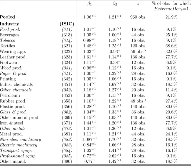
Table 2: Simple HME test - structural breakpoints

β1 β2 π % of obs. for which

ExtremeDevπ=1

Pooled 1.06>1 _1.21>1 _{960 obs. 21.9%}

Industry (ISIC)

Food prod. (311) 1.01=1 _1.10>1 _{16 obs. 9.1%}

Beverages (313) 1.05>1 _1.00=1 _{44 obs. 25.1%}

Tobacco (314) 0.98=1 _1.18>1 _{16 obs. 9.1%}

Textiles (321) 1.48>1 _1.25>1 _{120 obs. 68.6%}

Wearing app. (322) 1.03=1 _0.93a _{56 obs.}[ _32.0%

Leather prod. (323) 1.61>1 _1.14=1 _{136 obs. 77.7%}

Footwear (324) 1.11=1 _0.38a _{12 obs. 6.9%}

Wood prod. (331) 0.98=1 _1.12>1 _{16 obs. 9.1%}

Paper & prod. (341) 1.00=1 _1.22>1 _{28 obs. 16.0%}

Printing (342) 1.05>1 _1.06>1 _{16 obs. 9.1%}

Indus. chemicals (351) 1.14>1 _1.67>1 _{32 obs. 18.3%}

Other chemicals (352) 1.18>1 _1.27>1 _{20 obs. 11.4%}

Petroleum (353) 1.00=1 _1.15>1 _{16 obs. 9.1%}

Rubber prod. (355) 1.10>1 _1.22>1 _{48 obs.}[ _27.4%

Plastic prod. (356) 1.28>1 _1.10>1 _{140 obs. 80.0%}

Glass & prod. (362) 1.04=1 _1.33>1 _{36 obs. 20.6%}

Other mineral prod. (369) 1.15>1 _1.03>1 _{140 obs. 80.0%}

Iron & steel (371) 1.44>1 _1.20>1 _{136 obs. 77.7%}

Other metals (372) 1.01=1 _1.36>1 _{12 obs. 6.9%}

Metal prod. (381) 1.11>1 _1.21>1 _{44 obs. 24.1%}

Non-elec. machinery (382) 1.087=1 _1.70>1 _{32 obs. 18.3%}

Electric machinery (383) 0.84=1 _1.66>1 _{28 obs. 16.1%}

Transport equip. (384) 1.02=1 _1.41>1 _{28 obs. 16.1%}

Professional equip. (385) 0.72=1 _2.62>1 _{16 obs. 9.1%}

Other manuf. (390) 0.77a _1.42>1 _{32 obs. 18.3%}

Notes: a_{: significant at the 1% level.} =1_,>1_{: Significant at the 1% level, and respectively}

equal and greater than one at the 5% level. [_{: Breakpoint is not significant at the 10%}

level. Italics denote industries that exhibit a piecewise HME

We recall that the HME (if it exists) is stronger away from the symmetric equi-librium than near it. Sectoral estimations serve the principal purpose of verifying empirically this result for each industry. To this purpose, we test for parameter structural change in a simple linear HME estimation. In addition, this estimation allows also to identify the type of non-linearity characterizing each individual sector.

∆S,ikt = β1(1 − ExtremeDevπ)∆D,ikt+ β2(ExtremeDevπ)∆D,ikt, (10)

where ExtremeDevπ is a dummy variable that equals one if ∆D,iktbelongs to the π/2 smallest or the π/2 greatest values in the sample and zero otherwise. We test β1 6= β2 performing Wald tests for several values of π, then we consider the larger

value of Wald statistic as the most significant break point.12 _{Hence, the estimated}

critical value of π splits the data into three sub-groups: a group of observations that have small values of derived demand deviations, a group of large derived demand deviations, and a group of intermediate derived demand deviations. The two groups of extreme values of demand deviations are of identical size and we assume that the HME is of identical magnitude for both of them. The smaller is the estimated value of π the smaller is the size of these two groups of observations. The first three columns of Table 2 report the estimated values of β1 and β2 and the critical

values of π. The last column reports the percentage of observations for which

ExtremeDevπ = 1, that is the observations for which the slope is equal to β2.

The first row of Table 2 shows the results for the pooled data.13 _{We see that}

β2 > β1 > 1, which suggests that HME matters for all countries though more

strongly for extreme values of demand deviations. This is consistent with the smooth non-linearity found in the pooled estimation of equation (9).

The remaining lines of Table 2 report the results for each individual industry.14

Two industries (Footwear and Wearing apparels) can be associated to the CRS-PC paradigm. Footwear exhibits a smooth inverted HME (β1 ≤ 1 and β2 < β1),

but results for Wearing apparels are more ambiguous since the maximum-Wald test does not identify a significant breakpoint. Seven industries provide unexpected results. For six of them (Beverage, Textile, Leather, Plastics, Other mineral products, and Iron and steel) both β1 and β2 are larger than one, but β1 > β2. These

industries clearly exhibit a significant Home Market Effect but do not fit in any of the cases identified in the theoretical model. For Other manufacturing products the results are cannot be interpreted using the model: β1 < 1 but β2 > 1. The

other sixteen industries show results consistent with the IRS-MC paradigm. Four

12_{See Andrews (1993, 2003).}

13_{We increase π from 20 to 2000, using steps of 20 observations.}

14_{There are 175 observations for each of the 25 industries. We perform 42 regressions for each}

of them (Printing, Industrial chemicals, Other chemicals and Metal products) show a smooth HME (β2 > β1 > 1), and one (Rubber) exhibits a linear HME. Finally,

for the eleven remaining industries econometric results give evidence in favor of a piecewise HME (β2 > β1 = 1).

The eleven industries exhibiting a piecewise HME represent more than 62% of manufacturing production in our sample. Moreover, for all of them, the correspond-ing threshold values of π are rather small: the percentage of observations for which

ExtremeDevπ = 1 ranges from 9.1% to 20.6% and is 12.5% on average. This means

that the Home Market Effect influences the specializations in 62% of the manufac-turing activity of only about 12.5% of the countries on average.

5

CONCLUSION

We have eliminated the outside good from the model that used the HME to test trade theories. Our theoretical results confirm that the discriminating criterion based on the HME is robust to such model modification except in the special case of perfect substitutability between domestic and foreign production of the CRS-PC good combined with prohibitive trade costs for this good. This special case is never observed at the level of industry aggregation normally used in the empirical literature. It seems safe to conclude, therefore, that the HME remains a valid criterion with which to test trade theories. The robustness of the HME has another important implication. It implies that the outside good assumption, although clearly at odds with reality, does not affect qualitatively the results concerning international specialization and the direction of trade. Therefore, its pervasive use is justifiable on the ground of algebraic convenience. However, in the absence of the outside good, the HME is attenuated and may disappear in a subset of the incomplete specialization set. This is important because it implies that all results hinging on the HME (results concerning specialization, but also welfare results) should be taken with same caution since their actual magnitude is probably smaller than what is predicted by models which assume an outside good. Finally, the HME is found to be non linear. The non-linearity implies that the home market effect is more important for countries whose demand deviations are very different from the average than for countries whose demand deviations are close to the average. Therefore, the consequences of small demand shocks (be it due to preference shocks

or to public policy) are likely to have a much smaller (if any) impact on international specialization than what is predicted by models that assume an outside good.

Our empirical investigation strongly supports the non-linearity in both pooled and sectoral regressions. We find evidence of non-linearity in 16 sectors out of 25. Five of them exhibit the smooth non-linearity and eleven of them show the piecewise non-linear HME. The latter result tells us that although the HME exists, its economic importance is limited since it influences the specialization of a small number of countries (about 12.5 % of the sample).

We conclude by pointing at one other related issue concerning trade costs and the HME. The HME derived in the two-country model with outside good extends to the many-country model (with outside good) if it is assumed that countries are equidistant but it does not (in general) if countries are not equidistant. Behrens et al. (2004) explore this issue in great detail while keeping the assumption of the existence of an outside good that equalizes wages and offsets all trade imbalances. We have limited our analysis to the the two-country case but have complicated matters by eliminating the outside good. Ideally, one would like to see a tractable model with many non-equidistant countries and without the outside good, but this proves to be beyond mathematical tractability for the time being.

6

APPENDIX

6.1

Finite Elasticities: results from numerical methods

We want to find out the shape of the function SN(SL). We start by solving system

(1)-(8) for 3,645 (93_{· 5) different sets of parameters values. Each set consists of}

dif-ferent values assigned to the four parameters (σ, γ, τA, τM). We have set σ equal to

3, 4, 5, 7, and 8.16 _{For each of these values of sigma we let the other parameters take}

all possible combinations of values at intervals of 0.1 (nine values for each param-eter). We then approximate the function SN(SL) with the third-degree polynomial p (SL) =

3

X

i=0

ci(SL)i for each of the 3,645 different set of parameter values.17 We use

Chebyshev interpolation method which greatly outperforms Lagrange interpolation (see Judd, 1998). The approximation method gives the coefficients of p (SL) which,

through use of simple calculus, give us the shape of the unknown function. In fact, the first derivative of the polynomial is larger than one for any SLif c1−1₃(c2)

2

c3 > 1.

All simulations gave values of c1−1₃(c2)

2

c3 larger than one. Therefore SN(SL), as

ap-proximated by p (SL) is increasing in SLand its slope is larger than one in the entire

incomplete specialization set. The second derivative of the polynomial is positive, zero, or negative as SL is larger, equal, or smaller than −1₃c_c2₃. Thus, the function is

concave (convex) for values of SL smaller (larger) than −1₃c_c2₃ and it has an inflexion

point at SL = −1₃c_c2₃. Using the coefficients of the approximating polynomial the

inflexion point is found at SL ' 1/2 in all simulations (the greatest deviations from

1/2 occur at the sixth decimal digit). Therefore, SN(SL) has the shape represented

in Figure 1 in all the 3,645 simulations.

15_{Maple files associated with the mathematical appendix are available at:}

http://team.univ-paris1.fr/teamperso/crozet/matthieu.htm.

16_{These values of sigma are often used in numerical explorations of this class of models and}

are comparable to those resulting from gravity equation estimation. For instance, Head and Ries (2001) find a sigma equal to 7.9, Baier and Bergstrand (2001) find it equal to 6.43, Head and Mayer (2005) find it equal to 8, Hanson (2005) finds it equal to 4.9, and Broda and Weinstein (2006) find it equal to 4 among three-digit goods.

17_{Using a polynomial of a higher degree would increase the precision of approximation but would}

not give further qualitative information about the shape of the function SN(SL). We therefore

6.2

Perfect substitutability in the CRS-PC good: analytical

results

Since good A is homogenous across countries, consumers have a single demand for

A instead of separate demands for each country’s variety of A. This demand is: ai = (1 − γ) Yi/pAi , where pAi is the domestic price of A.18 We assume γ < 1/2 so

that the largest country produces both goods for any SL.

When there is trade in A we have either pA1= _τ1_ApA2(if country 1 is the importer

of A) or pA2 = _τ1_ApA1 (if country 1 is the exporter of A). Either one of these two

equations, plus (1)-(5) and (7)-(8), determine the fifteen endogenous. In particular, when country 1 is the importer of A we have:

SN (right) = φ2 MτAσ+1−τAφM+SL(τAσ−φM+τAφM−φ2MτAσ+1) τσ A−τAφM−φMτA2σ+φM2 τAσ+1+SL(τAφM−φM+φMτA2σ−φMτA2σ−1+φ2MτAσ−1−φ2MτAσ+1) , for any SL ∈ ³ SL, S is L ´ .

When country 1 is the exporter of A we have:

SN (lef t) = − ( −τ2 AφM+τAφM−φ2MφA+τAφM)SL+φ2MφA−τAφM (φ2 MφA+τA2φM−τAφM−τA2φ2MφA+τAφMφ2A−φMφ2A)SL−φ2MφA−τAφA+τAφM+φ2AφM, for any SL∈ ³ Sis L, SL ´ .

When there is no trade in A, domestic demand of A must be satisfied by domestic supply. Therefore, the market equilibrium conditions for A are:

A1 = (1 − γ) L1 (11)

A2 = (1 − γ) L2 (12)

The system composed of (1)-(4), plus (7)-(8) and (11)-(12) determines the fifteen endogenous. In particular, we have that SN = SL. Summing up, we have the

following piecewise relationship:

SN =       

SN (lef t), for any SL ∈

³

Sis L, SL

´

SL, for any SL ∈ [SL, SL]

SN (right), for any SL ∈

³

SL, S is L

´ (13) This is the expression plotted in Figure 2 for σ = 3, τA = 9, and τM = 7).19

18_{The subscript}

i to the A good now refers to the price or the output of that good in country i

and not, as in the Armington model, to the price or quantity of country i’s variety of A. Since σA

equals infinity we drop the subscript from σM to lighten notation. 19_{The expressions for S}

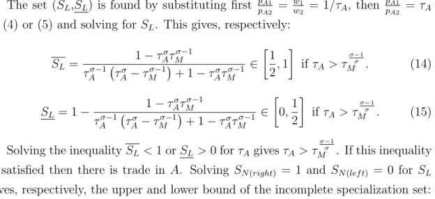
The set (SL,SL) is found by substituting first p_pA1_A2 = _ww1₂ = 1/τA, then p_pA1_A2 = τA

in (4) or (5) and solving for SL. This gives, respectively:

SL = 1 − τσ AτMσ−1 τ_Aσ−1¡τσ A− τMσ−1 ¢ + 1 − τσ AτMσ−1 ∈ · 1 2, 1 ¸ if τA> τ σ−1 σ M . (14) SL = 1 − 1 − τσ AτMσ−1 τ_Aσ−1¡τσ A− τMσ−1 ¢ + 1 − τσ AτMσ−1 ∈ · 0,1 2 ¸ if τA> τ σ−1 σ M . (15)

Solving the inequality SL< 1 or SL> 0 for τAgives τA> τ

σ−1 σ

M . If this inequality

is satisfied then there is trade in A. Solving SN (right) = 1 and SN (lef t) = 0 for SL

gives, respectively, the upper and lower bound of the incomplete specialization set:

Sis_L = φMτ 1+σ A − τA −τA+ φ2_M − φMτ_Aσ+ φMτ_Aσ+1 ∈ µ 1 2, 1 ¶ if τA > τ σ−1 σ M . (16) Sis_L = 1 − φMτ 1+σ A − τA −τA+ φ2M − φMτAσ + φMτAσ+1 ∈ µ 0,1 2 ¶ if τA> τ σ−1 σ M . (17)

6.3

Pooled regressions: Robustness checks

Table 3 presents several of robustness checks of the result presented in Table 1. Table 3: Pooled regressions - Robustness tests

Dependent Variable: ∆S (production deviation) - OLS estimates

(1) (2) (3) (4) (5) Values OECD ΦG ijk ∆D 1.168>1 1.131>1 1.146>1 1.145>1 1.053>1 (0.021) (0.025) (0.014) (0.014) (0.022) ∆D.|∆D| 0.310b 0.081 0.261a 0.268a 0.658c (0.133) (0.129) (0.074) (0.075) (0.374)

Fixed Effect No No Year Indus. No

Nb. Obs. 4375 2800 4375 4375 4375

R2 _{0.880 0.879 * * 0.507}

Notes: SDis the computed derived demand deviation. a,b,c: Respectively

signif-icant at the 1%, 5% & 10% levels. =1_,>1_{: Significant at the 1% level, and}

respectively equal and greater than one at the 5% level. Robust standard er-rors in parentheses. ∗ We constrain the sum of the fixed effects to be equal to zero; R2 _{are not calculated.}

take the derivatives of dSN (right) dSL and

dSN (lef t)

dSL . It is easily verified that, if τA= 1, then SN (rigth)=

SN (lef t)= 12+ 1+φM 1−φM ¡ SL−1₂ ¢ exactly as in Helpman-Krugman (1985).

Column (1) reports the estimates of the model using values of production and demand rather than volumes. In column (2), we show the estimates obtained from the database restricted to OECD countries. Columns (3) and (4) display the es-timates with year and industry fixed effects respectively. Finally, in column (5), we consider an alternative mesure of trade freeness, Φijkt. As Davis and Weinstein

(2003), we first perform a gravity estimation for each industry; then the coefficients of this regression are used to compute the bilateral trade barrier, ΦG

ijk.

References

[1] Amiti M. (1998) “Inter-industry trade in manufactures: Does country size mat-ter” Journal of International Economics 44: 231-255.

[2] Andrews D.W.K. (1993) “Test for Parameter Instability and Structural Change with Unknown Change Point” Econometrica 61 (4):821-856.

[3] Andrews D.W.K. (2003) “Test for Parameter Instability and Structural Change with Unknown Change Point: A Corrigendum”, Econometrica 71 (1): 395-397. [4] Armington, P.S. (1969) “A theory of demand for products distinguished by

place of production” IMF Staff Papers 16: 159-176.

[5] Baier S.L. and J.H. Bergstrand (2001) “The Growth of World Trade: Tariffs, Transport Costs, and Income Similarity”, Journal of International Economics 53(1):1-27.

[6] Behrens K., A. Lamorgese, G.I.P. Ottaviano and T. Tabuchi (2004) “Testing the ‘Home Market Effect’ in a Multi-Country World: A Theory-Based Approach”. CEPR Discussion Paper 4468.

[7] Broda C. and D.E. Weinstein (2006) “Globalization and the Gains from Vari-ety”. The Quarterly Journal of Economics 121(2): 541-85.

[8] Br¨ulhart M. and F. Trionfetti (2005) “A Test of Trade Theories when Expen-diture is Home Biased” CEPR Discussion paper 5097.

[9] Davis, D.R. (1998) “The Home Market, Trade and Industrial Structure”

Amer-ican Economic Review 88: 1264-76.

[10] Davis, D.R. and D.E. Weinstein (1999) “Economic Geography and Regional Production Structure: an empirical investigation” European Economic Review 43: 379-407.

[11] Davis, D.R. and D.E. Weinstein (2003) “Market Access, Economic Geogra-phy and Comparative Advantage: an Empirical Test” Journal of International

Economics 59: 1-23.

[12] Feenstra, R. C., J. A. Markusen and A.K. Rose (2001) “Using the Gravity Equa-tion to Differentiate Among Alternative Theories of Trade”Canadian Journal

of Economics 34: 430-47.

[13] Feenstra R. C, Romalis J. and Schott P. K. (2002) “U.S. Imports, Exports, and Tariff Data, 1989-2001”. NBER Working Paper 9387.

[14] Hanson H.G. (2005) “Market Potential, Increasing Returns, and Geographic Concentration” Journal of International Economics 67: 1-24.

[15] Hanson, H.G. and C. Xiang (2004) “The Home Market Effect and Bilateral Trade Patterns” American Economic Review 94: 1108-1129.

[16] Head, K. and T. Mayer (2004) “The Empirics of Agglomeration and Trade” CEPR Discussion Paper 3985 and also Ch. 59 in J.V. Henderson and J-F. Thisse (eds), Handbook of Urban and Regional Economics, Vol. 4. North Holland. [17] Head, K. and T. Mayer (2006) “Regional Wages and Employment Responses to

Market Potential in the EU” Regional Sciences and Urban Economics 36(5):573-95.

[18] Head, K., T. Mayer and J. Ries (2002) “On the Pervasiveness of the Home Market Effects ” Economica 69: 371-90.

[19] Head, K. and J. Ries (2001) “Increasing Returns Versus National Product Dif-ferentiation as an Explanation for the Pattern of US-Canada Trade” American

Economic Review 91: 858-876.

[20] Helpman, E. and P. Krugman (1985)Market Structure and Foreign Trade, MIT Press, USA.

[21] Holmes, T. J. and J. J. Stevens (2005) “Does home market size matter for the pattern of trade?” Journal of International Economics 65: 489-505.

[22] Judd K. (1998) “Numerical Methods in Economics ” MIT Press.

[23] Krugman, P.R. (1980) “Scale Economies, Product Differentiation, and the Pat-tern of Trade” American Economic Review 70: 950-9.

[24] Laussel, D. and T. Paul (2007), “Trade and the location of industries: Some new results ” Journal of International Economics 71: 148-166.

[25] Lundb¨ack, E. and J. Torstensson (1998) “Demand Comparative Advan-tage And Economic Geography In International Trade: Evidence From The OECD”Weltwirtschaftliche Archiv 134: 230-49.

[26] Mayer, T. and S. Zignago (2005) “Market Access in Global and Regional Trade”CEPII working Paper 2005-02.

[27] Trionfetti, F. (2001) “Using Home-Biased Demand to Test for Trade Theories”

Weltwirtschaftliches Archiv 137: 404-426.

[28] Weder, R. (1995) “Linking Absolute and Comparative Advantage to Intra-industry Trade Theory”Review of International Economics 3(3):342-354. [29] Weder, R. (2003) “Comparative Home-Market Advantage: An Empirical

Anal-ysis of British and American Exports”Weltwirtschaftliches Archiv 139: 220-247. [30] Yu, Z. (2005) “Trade, Market Size, and Industrial Structure: the Home Market