Analysis of peak characterization and data alignment of a differential mobility spectrometer for the discovery of TB biomarkers in human breath

Analysis of Peak Characterization and Data

Alignment of a Differential Mobility Spectrometer

for the Discovery of TB Biomarkers in Human

Breath

by

Amy Yuen-Lee Tang

MASSACHUSETTS INSTITUTE

OF TECHNOLOGY

NOV 13 2008

LIBRARIES

Submitted to the Department of Electrical Engineering and Computer

Science

in partial fulfillment of the requirements for the degree of

Master of Engineering in Electrical Engineering and Computer Science

at the

MASSACHUSETTS INSTITUTE OF TECHNOLOGY

December 2007

@

Massachusetts Institute of Technology 2007. All rights reserved.

Author ...

DepartmentV6 Electrica

lneering and Computer Science

December 20, 2007

... ... .... .. . ... ... .... ...

Roger

G.

Mark

Distingushed Profesor in Health Science & Technology

Thesis Supervisor

Certified by

Nirmal Keshava

Draper Laboratory

-Supervisor

Ferry Orlando

IlEad--o

Technical

S aff,

...

.

Accepted by

Chairman, Department Committee on Graduate Students

Abstract

Biomarkers have become a growing field for disease research and diagnostics. For the infectious, deadly disease, tuberculosis (TB), the discovery of effective TB biomarkers in the human breath may enable the development of a cheap, fast, and accurate TB diagnostic to fight against this epidemic. The Charles Stark Draper Laboratory is em-ploying a differential mobility spectrometer (DMS), in order to identify key biomarkers for TB. Biomarker candidates appear as peaks in the DMS sensor data at particu-lar retention times and DC compensation voltages. Possible biomarkers are identified through well-known classification techniques, K-nearest neighbors and support vector machines. This research is focused on the development of a toolbox that will aid in the discovery and in-depth understanding of the TB breath biomarkers. This thesis demonstrates the algorithms and capabilities of peak quantification, characterization, RIP-based alignment, and siloxane-based alignment on protein and bacterial sensor data, including those from initial Mycobacterium tuberculosis samples. The results show that siloxane-based alignment with high-intensity peak landmarks effectively increase DMS peak stabilities and signal-to-noise ratios. These new tools will be important for the analysis of specific TB biomarker candidates as our group at the Charles Stark Draper Laboratory receive more samples of M. tuberculosis.

Acknowledgements

I would like to thank Nirmal Keshava, Professor Roger Mark, Meredith Gerber, and Professor Collin Stultz, who have guided and supported me throughout this thesis endeavor. Your sharp minds and questions have provided a collaborative setting for my Master's research. I thank the Charles Stark Draper Laboratory for the financial support through a Draper Lab Fellowship. It was exciting to present a poster on my research at the Broad Institute TB conference.

I would like to thank my loving and beautiful sister, Cynthia, and my enthusiastic and caring parents, Alex and Mon Li. These strong pillars in my life have grounded and sustained me.

To all my wonderful friends during graduate school - Sandra, Philip, Gaurav, So-han, Priscilla, Manway, Tushar, Gireeja, Shirley, Anindya, Madhu, Elizabeth, Indy, Clarence, Sonia and Gemma - your passions, intelligence, hard work, generosity, and kind hearts have touched and inspired me. Thank you also for all the laughs. To my ballroom dance partner, David Xie, thank you for the good times and practices; dancing has become such an important form of self-expression, exercise and freedom for me. Above all, I want to thank God for giving me life, joy, grace, and incredible opportunities.

Contents

1 Introduction

1.1 Motivation . ...

1.2 DMS Sensor and Processing . . 1.3 Biomarkers in the DMS . . . .

1.4 Peak Processing and Alignment

2 Overall Hardware and DMS 2.1 Overall Hardware ... 2.2 DM S .. ... ... ... . . 2.2.1 Background ... 2.2.2 Drift Effects ... 2.2.3 DMS Input . . . . 2.2.4 DMS Output ... 2.2.5 Detector Polarity . . .. 2.2.6 RIPs ... 2.2.7 Siloxanes ... 3 Peak Characterization 3.1 Peak Quantification ...

3.1.1 Results on Human Breath . . . . . 3.2 Peak Characterization ...

3.2.1 Definition of Peak Location, Width, 3.2.2 Reporting Values ...

and Intensity

3.2.3 3.2.4 Results on Isoprene ... Results on Bacteria ... 4 Alignment Investigation 4.1 SN R . . . . 4.1.1 Synthetic Exercise: Investigate the SNR . . . . 4.2 RIP-based Alignment ...

4.2.1 Results on BSA, OVA, and Water . . . . 4.3 Siloxane-based Alignment . . . .

4.3.1 Peak Normalization ...

4.3.2 Self-Alignment and Normalization . . . . 4.3.3 Results on M. smegmatis ...

4.3.4 Results on M. tuberculosis . . . .

5 Conclusions

5.1 Overall Results of RIP and Siloxane-based Alignments 5.2 Future W ork ... 35 . .. . 35 . . . . 38 . .. . 42 . . . . 42 . . . . 47 . . . . 48 . . . . 48 . . . . 51 . . . . 65 67 67 68

List of Tables

3.1 _{Peak quantification of human breath with 3 extraction times: 5, 10,} and 20 m inutes . . . .. . . . . . 19

4.1 RIP-based alignment (by first RIP) for BSA, OVA, and water. Aligned and unaligned data on the first and second RIP. . ... 44 4.2 Two BSA peaks are RIP-aligned; however the standard deviation has

List of Figures

1-1 Block Diagram of Signal Processing Approach . ... 4

2-1 An example of the DMS output. The color bar (z-axis) is the pixel intensity in unit of detector response (DR). . ... . 5 2-2 Experimental Hardware Apparatus . ... 7 2-3 DMS principles. Yellow and green ion movements collide into

elec-trodes and neutralize. The blue ion movement reaches the detectors.. 8 2-4 Standard Bacteria Growth Curve . ... . 11

2-5 The siloxane landmarks are wide intense peaks from inert compounds that are consistently released from the SPME fibers... 13

3-1 Block diagram of peak quantification ... . . . . 16 3-2 Peak counting of human breath. Threshold and n factor are 0.0050

and 0.300 respectively. ... ... 18 3-3 Number of more intense and wider peaks for 10 extractions for the

depletion study. The threshold and n factor of the negative spectrum are 0.0078 and 0.0068. ... 20 3-4 Number of large peaks for ten different extractions. The threshold and

n factor of the positive spectrum are 0.008 and 0.007. . ... 21 3-5 Number of more intense and wider peaks for 10 extractions (depletion

study) are presented in box and whisker plots. . ... . 22 3-6 Number of general peaks for ten rounds of extractions. The threshold

3-7 Number of general (small and large) peaks for ten different extractions. The threshold and n factor of the positive spectrum are 0.0066 and 0.0056. 24

3-8 Number of general peaks for ten extractions presented in box and whisker plots. ... ... . ... .. 25

3-9 The peak position is indicated by an orange arrow and the peak width by an orange line. This y-axis is the marginal or weight value. .... 26

3-10 Zoomed-in DMS sensor data: 1 isoprene peak (205.8s) and 4 siloxane peaks... ... . 27

3-11 Summary plot of peak parameter characterization of isoprene and silox-anes for time dimension. ... ... 28

3-12 Summary plot of peak parameter characterization of isoprene and silox-anes for voltage dimension. ... ... 29

3-13 DMS sensor data taken from the lag phase of M. smegmatis in April 2007. (Color bar is the z-dimension of intensity in DR units). RIP line is absent. ... ... 29

3-14 Summary chart of peak parameter characterizations for a siloxane and a high-intensity peak (peaks 1, 2). ... . 30

3-15 Summary chart of peak parameter characterization for two siloxanes (peaks 3, 4) ... ... 30

3-16 Summary chart of peak parameter characterization for two low-intensity peaks (peaks 5, 6). ... ... ... . . 31

3-17 Peak intensity of 4 peaks for group 2. No correlation is visually observed. 32

3-18 Individual peak profile of a siloxane peak #1. . ... . 33

3-19 Individual peak profile of a low-intensity peak #5. The Vc marginal exhibits no peak shape. ... ... ... . . 33

3-20 Low-intensity peak #5: Gaussian model and individual peaks. ... 34

4-1 The Gaussian model peak (average) and the original peaks from the bacteria DMS data. ... ... 36

4-2 Synthetic peak exercise with 1:1 ratio of the Gaussian model peak and moving peak maximum intensity height . ... 38

4-3 Synthetic peak exercise with 1:2 ratio of the Gaussian model peak and moving peak maximum intensity height . ... 40

4-4 Synthetic peak exercise with 1:4 ratio of the Gaussian model peak and moving peak maximum intensity height . ... 41

4-5 Example of RIP-based alignment of file 33 to file 1 (reference) to match the first reactant ion potentials ... .. ... . 43

4-6 Investigate the alignment by first RIP. The pink line is the first RIP. The blue line is the second RIP. ... .. 43

4-7 RIP-based alignment for one BSA biomarker. Its voltage location has random variability but its time position shows a drifting trend. For the aligned data, the BSA biomarker exhibits a higher standard deviation which is destabilization, an undesirable effect. . ... . 45

4-8 Effects of normalization and shifting (self-alignment). Shifting affects the peak's position, and normalization affects the peak's height. Shift-ing alone generally increases the SNR more than normalization alone. The majority of peaks generated the highest SNR increase with com-bined normalization and shifting. ... . . . 49

4-9 Effects of normalization and shifting for a siloxane peak (peak 1, file 5), shown for time dimension. Gaussian model: height of 0.125 DR, center of 290.4 s. In this case, the normalization and shift successfully matched this peak to its Gaussian model. . ... 50

4-10 DMS sensor data taken from the lag phase of M. smegmatis in April 2007. (Color bar is the z-dimension of intensity in DR units). ... 51

4-11 Summary of the average peak characterizations in retention time for

M. smegmatis over thirteen files. * indicates the peak. Left y-axis

refers to peak half-width and standard deviations in seconds. Right y-axis refers to intensity (DR) . ... ... ... 52

4-12 Summary of average peak characterizations in compensation voltage for M. smegmatis over thirteen files. * indicates the peak. Left y-axis refers to peak half-width and standard deviations in voltage. Right y-axis refers to intensity (DR)... .. 53 4-13 Exact values of six peak characterizations for M. smegmatis. ... 54 4-14 Peak profile of peak 1 (siloxane) from M. smegmatis, April 2007 for

run 2. Included are marginal distributions, peak characterizations and a 3D visual. This particular siloxane has a very high max intensity, 0.140 DR, while the average max intensity is 0.125 DR. ... . 55 4-15 Peak profile of peak 2 (HI peak). ... 56 4-16 Peak profile of peak 3 (siloxane) ... 57 4-17 Peak profile of peak 4 (siloxane). This peak is wider than the Gaussian

model. ... 58 4-18 Peak profile of peak 5 (LI peak). The Vc marginal profile shows a

non-peaky shape but a random distribution. . ... 59 4-19 Peak profile of peak 6 (LI peak). The time marginal profile is taken

over a smaller range, because there were other peaks on both sides. 60 4-20 Siloxane-based alignment improves SNR for six DMS peaks. The

brown line shows no alignment. The red line shows the overall greatest increase in peak SNRs; therefore the alignment to reference peak 2 is most successful in aligning DMS peaks. . ... 61 4-21 SNR after alignment based on different reference peaks. Top row is

peak SNRs under no alignment. Blue box is the largest SNR for that particular peak (in the column). Circled regions indicate peak SNRs with the highest increase, resulting from alignment based on siloxanes and another high-intensity peak (peaks 2-4). . ... . 62 4-22 Change in SNR after alignment. Blue box is the largest SNR increase

for that particular peak (in the column)Circled regions indicate highest increase in SNR, which occurred after alignment based on siloxanes and another HI peak. ... 62

4-23 Zoomed view of DMS sensor data from M. tuberculosis, 2007. Three high-intensity peaks are selected as landmarks for siloxane-based align-m ent... . . . .. . 65 4-24 Alignment using three reference HI peaks in the M. tuberculosis data.

The increased, aligned SNR values of the peaks indicate that alignment by HI peaks is effective in peak stabilization of DMS sensor data. . . 66

Chapter 1

Introduction

1.1

Motivation

Tuberculosis (TB) is a world-wide health problem. One third of the world population (2 billion people) have the latent form of M. tuberculosis in their body, 15 million have active TB, and 1.7 million people died of TB in 2004. TB is the second leading infectious disease, and the leading cause of death for people with HIV or AIDS. Every second a new infection occurs, as reported by the World Health Organization [20]. One major cause of this TB epidemic is the inadequacy of effective TB diagnostics for third-world countries. Poor nations are limited to the diagnostic methods developed 100 years ago, nearly when TB was first identified by Dr. Robert Koch in 1882. Cur-rent gold standards for TB diagnosis are far too expensive. Ineffective TB diagnosis and non-rigorous drug compliance is causing the fast growth of multi-drug resistant (MDR) and extreme-drug resistant (XDR) strains of TB in Africa, Russia, and South America. The emergence of a portable, low-cost TB diagnostic is a high priority for the fight against the TB epidemic.

1.2

DMS Sensor and Processing

The Charles Stark Draper Laboratory and Sionex have developed a portable, highly sensitive device called the differential mobility spectrometer (DMS) for chemical

de-tection. This device is currently used for applications such as biological warfare and explosives surveillance. In order to meet the need for novel diagnostic modalities, we have adapted this tool for TB biomarker discovery, in order to develop a potential breath analysis device. The DMS instrument must be coupled with signal processing methods to extract information and to characterize key peaks. K-nearest neighbors (KNN) and support vector machines (SVM) are machine-learning classification meth-ods to determine key features in the DMS sensor that can lead to the discovery of biomarkers.

1.3

Biomarkers in the DMS

A biomarker is a general term for an indicator, such as a genetic marker, an antibody, or a chemical substance, that signifies the presence of a particular agent or diseased state [12]. Diabetes, heart attacks, and kidney injury can be diagnosed by increased levels of acetone, pentane, and ammonium respectively [16] [6]. It is well-established that increased levels of methylethylketone, tolualdehyde and oxepanone are detected in lung cancer patients [14]. In this research, the biomarkers are key volatile organic compounds (VOCs) that appear exclusively or in elevated levels for the diseased state. Phillips et. al [18] have identified 3,000 VOCs in the human breath. The gases present in the exhaled breath are nitrogen (75%), oxygen (16%), carbon dioxide (4%), water (4%), and argon (0.9%), which make up a total of 99.9% of the breath. The remaining volatile organic compounds are measured as parts per million (ppm) or parts per billion (ppb). The most abundant remaining VOCs in the breath are

isoprene (12 ppb - 580 ppb), acetone (1.2 ppb - 1880 ppb), ethanol (13 ppb - 1000

ppb), and methanol (160 ppb - 2000 ppb) as reported by Phillips [19].

The DMS sensor data exhibit multiple peaks for the VOCs of human breath. However, not all these peaks are biomarkers. In the simple case, a biomarker is present in one class and absent in the other. In another case, the biomarker is in elevated levels for one class and in lower levels for another class. A third case is a distinct biomarker signature, which is a composition of several VOCs that all must

exhibit elevated levels.

Phillips et al. [17] have reported possible TB breath biomarkers from clinical TB patient trials in New Jersey. They concluded that active pulmonary tuberculosis alters normal VOCs found in the human breath. The oxidative stress on Mycobacterium tuberculosis produces either elevated amounts and unique forms of VOCs, such as methylated alkanes and branched benzenes. These suspected TB biomarkers give clinical evidence that significant TB biomarkers may exist for active TB. With the use of Gas-Chromatography/DMS and Gas-Chromatography/Mass-Spectrometry in our research, it will be possible to do our own investigation of TB breath biomarkers.

1.4

Peak Processing and Alignment

Initially, classification is used to identify the top DMS pixels that effectively distin-guish between the diseased and non-diseased states. The ideal situation is that top DMS pixels would appear as a peak in the diseased state and a non-peak in the non-diseased state, resulting in possible VOC biomarkers for TB. Upon closer inves-tigation, many top pixels were arbitrary pixels that, by chance, performed well in the classification. These pixels basically have no physical meaning or relevance to possible biomarkers. The research objectives are to align the DMS data, and develop peak characterization methods that serve two purposes: verify that a top pixel is ac-tually a peak in the diseased state and to characterize authentic top peaks by precise locations, sizes and intensity heights.

The overall process used by my team is described in Figure 1-1. This research focuses on the peak quantification, characterization, robustness quantification, land-mark selection, and alignment. The signal processing algorithms combined with the DMS and mass spectrometer can lead to the discovery of disease-specific VOCs in the breath to be uses as biomarkers for TB diagnosis.

Raw .CSV Data Ii-I Ii-I 'I

Figure 1-1: Block Diagram of Signal Processing Approach

_,c--Chapter 2

Overall Hardware and DMS

This chapter describes the overall hardware apparatus and the DMS sensor: inputs, outputs, detector polarities, drift effects, RIPs, and siloxanes. This thesis research focuses on the DMS output to identify TB biomarkers by signal processing, as shown in Figure 2-1.

Retention Time (s)

Figure 2-1: An example of the DMS output. The color bar (z-axis) is the pixel intensity in unit of detector response (DR).

2.1

Overall Hardware

The hardware apparatus involves a gas chromatograph (GC), a differential mobility spectrometer (DMS), a mass spectrometer (MS), and a computer. The overall setup and device settings are shown in Figure 2-2. The sample material is collected by fibers. If the sample is a gas, it is stored within TedlarTMBags and collected directly by the fibers. If the sample is a liquid, it is stored in a vial container and the headspace, which is the gaseous phase above, is collected, see Figure 2-2.

A holder storing the SPME fiber is placed into the injection port of the GC autosampler. The sample enters the cryogenic region (-125°C) to initially separate compounds. The sample runs through a GC column, which consists of a stationary and mobile phase. The stationary phase is a liquid in the column, and the mobile phase is a nitrogen carrier gas. The mobile phase moves the sample through the stationary phase within the column. Compounds with less affinity to the stationary phase will move through the column and elute, while compounds with high affinity stay behind and elute at later times. Half of the sample runs through the DMS, which is a sensor that performs rapid detection of biological and chemical compounds up to sensitivity of parts per trillion (ppt) [15]. The DMS can be used to identify the existence of biomarkers. The other half of the sample enters the MS, a common technique to determine the chemical identities of compounds. The MS is used to determine the chemical identities of the biomarkers.

2.2

DMS

2.2.1

Background

A recent version of the DMS was developed at the Charles Starker Draper Labora-tory in Cambridge, Massachusetts. The promise of this sensor led to the emergence of a new company, the Sionex Corporation, which now manages the sales of the in-strument. The market name of this DMS sensor is MicroDMxTM. The other name for the DMS is the field-asymmetric ion mobility spectrometer (FAIMS), which is

us AGemr rM

izlbnge: 39-300

SmRaceTupumube : 150-C DeIchrTetpeLuw : 230C

Sum IBle: 5.25sec

no=

room

Sample collected by SPME

$Pl Fier: SM0 ?

SP F : ecrTMTarue: 250C;

Oim Pmgm: 50 *C (2 an hold) inasmd coi on to 170C (3 mn hdkl)at 4 'CaM and Ien I

230C at 150C hain (PDMSWICaiu) CanierGus: Heh,

E, cnu Tie, 35 i _{FlowRte: 2mL}

Cryjglc Tespem e : -125'C

I

Figure 2-2: Experimental Hardware Apparatus

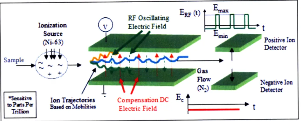
different than an ion mobility spectrometer (IMS), which separates ions by mobility using only one constant electric field. The IMS cannot separate most VOCs. For the DMS, the ions are separated by mobility using an asymmetric oscillating electric field and a constant electric field. The principle of DMS is related to a quadrupole mass spectrometer, except that it measures mobility and not the mass-to-charge ratio [8].

The input sample travels from the GC into the DMS, where the compounds are first uniformly ionized by a radioactive Nickel-63 source. The ions are projected into motion by a carrier nitrogen gas. The ions drift through an ion filter region, or drift tube, which is the main feature of the DMS system. The ion filter region is found between two parallel, Faraday electric plates. One plate applies an asymmetric,

os-cillating electric field, and the other provides a constant DC compensation voltage.

s3FibI

Data

Acquisition

SVAC-VaMd Skar Co Dieia ulLuge( r OO1100V

ConpauUakenHugeAlmg : -3DVb10 OV FlowtRab: 400 man ScmRbe: 125 Hz DifGaG: Nkagen r J I

Somce (Ni-63)_{i± -,}

R Oscnating ER )

Ioization ) Electric Field Lj

Positive Ion

Detector

Sample _ I I

Gas

Fl%-Aow Negative Ion

M-1kl~lllc

S / IE _c " ' " ueecra

Ion Tr~ectories Compensation DC ET

BaseMob&iies Electric Field

Figure 2-3: DMS principles. Yellow and green ion movements collide into electrodes and neutralize. The blue ion movement reaches the detectors.

Both electric fields are applied perpendicularly to the ion filter direction. The os-cillating field can reach radio frequencies up to 1000 Hz and therefore referred to as the radio-frequency or dispersion voltage [4]. In Figure 2-3, the plot of ERF displays the asymmetry of the oscillating field, where the waveform consists of a high-field portion Emax for time length tl and a low-field portion Emin for time length t2. The

ion mobility, K, significantly changes under the high-field compared to the low-field portion. This difference in ion mobility is AK:

AK = K(Emax) - K(Emin) (2.1)

As the ion drifts through the tube, the ions alternately get pulled toward one plate during the low-field portion and toward the other plate during the high-field portion, causing the bent motion of the ions (see yellow, blue, and green lines in Figure 2-3). The net distance toward one plate depends on the sign of AK. If the net distance is enough, the ions collide into a plate (yellow and green lines), neutralize, flow through the the tube, and not trigger the detectors. In order for ions with a given AK to remain in the center of the tube, a constant compensation voltage must be applied

so that ions can reach to the electrode detectors without becoming neutralized. This second electric field reverses, or compensates, for the net ion displacement, so that the ions are detected (blue line).

Eiceman et al. [10] have derived an equation for the total displacement, Y, of an

+ +/ /'

ion in the y-direction toward a plate under the following condition of the oscillating field:

Emaxj x tl = Emini x t2 (2.2)

These conditions simplify the Y equation to demonstrate the general effect of the variables. The total displacement, Y, of an ion in the y-direction toward a plate is

AKEmaxVD

Y = (2.3)

where AK is the difference in ion mobility between electric field strengths, the

Emax is the maximum electric field strength, V is the volume of ion filter region (area

of plate x height of filter), D is duty cycle where the electric field is in "up" state, and Q is the volume flow rate of the carrier gas. A greater displacement corresponds to a greater (in absolute value) necessary compensation voltage to bias the ions to move through the filter without contacting either plate. As the carrier gas flow rate

Q increases, the ions travel further along in the horizontal direction, so that the

absolute value of compensation voltage decreases. Additionally, as Emax under these conditions increases, the absolute value of compensation voltage must increase.

If an ion passes through the filter region, it becomes registered by either the posi-tive or negaposi-tive ion detector. The posiposi-tive electrode attracts the position ions and vice versa. The electrode measures the ion amount by a current that is then converted into intensity with units of detector response, DR. The oscillating field remains unchanged, while the sensor runs systematically through a range of compensation voltages such as from -30 V to +10 V.

2.2.2

Drift Effects

The causes of drifts for the DMS sensor are the appearance of a moisture level from water or changes in temperature, pressure, gas flow rate, maximum electric field strength, volume of the ion filter and other factors [5] [10]. These factors effect the mobility of the ions which then require slightly different compensation voltages

to reach the detectors. Eiceman et al. [11] showed that a moisture level causes clustering, which changes the compensation voltage and increases retention time due to the increased size. The normally inert nitrogen gas interacts with very few ions to cause clustering. Clustering has the strongest effect in extremely high and low electric field strengths. Barnett et al. [2] demonstrated that fluctuations in the carrier-in and carrier-out gas flow rates affect the RIPs and peak widths. The dispersion voltage of the carrier gas affects the compensation voltage. The effective volume of the ion filter can be reduced by any lack of cleanliness of the filter. Device fluctuations affect the general displacement equation, see Equation 2.3, by Eiceman et al. The variables of this equation include the difference in ion mobility between electric field strengths (AK), the maximum electric field strength (E,,max), the volume of ion filter region (V), duty cycle where the electric field is in "up" state (D), and the flow rate (Q). Any changes of these variables will affect the ion displacement in the DMS.

2.2.3

DMS Input

The DMS system was tested on these sample materials. The temperature, pressure or carrier gas flow rate may have been adjusted for optimal conditions.

* Human Breath

The breath sample originates from two human subjects, who do not have TB. These samples are used to begin detection of VOCs in the human breath.

* Bovine Albumin Serum (BSA) and Ovalbumin (OVA)

BSA and OVA are two proteins commonly used in research due to their low cost, stability and availability in large quantities. BSA is purified from bovine blood and weighs 66 kDa. OVA is found in egg white, a byproduct of the chicken industry, and weighs 45kDa.

* Isoprene

Isoprene (2-methylbuta-1,3-diene) is a commonly standard. Isoprene is a color-less, highly flammable liquid at room temperature. Isoprene is used to evaluate the repeatability of biomarkers and drifting effects in the DMS.

* Mycobacterium smegmatis

M. smegmatis is used as a simulant for M. tuberculosis. Both bacteria belong to

the genus Mycobacterium. M. smegmatis is non-pathogenic and often used for research. We analyzed the three growth phases of the bacterium, see Figure 2-4. We investigated for key biomarkers that can differentiate among the different

growth phases.

* Mycobacterium tuberculosis

The Massachusetts State Lab cultured M. tuberculosis, which is pathogenic and leads to the tuberculosis disease in animals. State lab technicians performed the extraction and returned SPME fibers, which were injected into the autosampler via an injection port, resulting in no exposure of M. tuberculosis to the open air. M. tuberculosis living in the human lung may produce very weak signals in the human breath; therefore we decided to use the bacterium directly for stronger signals to first identify TB biomarkers before using human breath of TB patients.

Figure 2-4: Standard Bacteria Growth Curve

2.2.4

DMS Output

The DMS data output consists of a file of pixels. Each pixel is a data point with three parameters: compensation voltage (volt), retention time (second), and intensity (detector response, DR). The detection of ions are displayed as peaks in the DMS data output, as seen in Figure 2-1. The DMS data are stored in a comma-separated values (CSV) format, which is a tabular form that is accessible by Microsoft Office Excel. The file translation process involves the import of CSV files into Mathworks

C

A: Lag S AN =8 B: Exponential

MATLABTMsoftware. A data file is stored in a MATLAB variable in 2-dimensional matrix form. Multiple files can be stored in a MATLAB variable as a 3-dimensional matrix in the format of a cube.

2.2.5

Detector Polarity

Every DMS run produces two sets of data associated to the positively and negatively charged detectors. The negatively charged detector attracts the positive ions and gen-erates the positive ion spectrum, such as the one shown in Figure 2-1. The positively charged detector attracts the negative ions and generates the negative ion spectrum.

2.2.6

RIPs

In the DMS output, the OVA, BSA, and water samples exhibit first and second reactant ion potential (RIP) landmarks in the positive DMS spectrum, see Figure 2-1. The locations of the RIPs are -16.0 V and -20.5 V, and these RIPS can be used for alignment. Occasionally the negative DMS spectrum exhibits a RIP at -20.5 V. The nitrogen carrier gas produces these RIPs. Nitrogen is an inert gas that normally does not interfere with other compounds. For the bacteria and human breath, the experimental methods were modified to remove the RIP landmarks from the data. The RIP lines are used to perform linear alignment in the voltage dimension.

2.2.7

Siloxanes

Like the nitrogen carrier gas, the siloxanes are inert compounds that do not interact with the compounds of the sample. Siloxanes are organosilicon compounds with empirical formula R2SiO, where R is an organic group, such as [SiO(CH3)2] where

n > 4, and its name is derived from the words silicon, oxygen and alkane. The siloxanes are released from the solid-phase microextraction (SPME) fibers used to collect human breath or bacterium's headspace. The elution times of three identified siloxanes are 294.6 s, 468.0 s, and 738.0 s, displayed in Figure 2-5. Siloxanes serve

Retention Time (s)

Figure 2-5: The siloxane landmarks are wide intense peaks from inert compounds that are consistently released from the SPME fibers.

as effective landmarks to align data. Other high-intensity peaks, as seen between siloxane peaks in Figure 2-5, may also serve as potential landmarks for alignment.

Chapter 3

Peak Characterization

3.1

Peak Quantification

The peak counting algorithm is a useful tool for estimating the maximum number of biomarkers in the DMS output. In order to build a breath diagnostic, human breath samples are run to measure the number of peaks that may correspond to VOCs. The peak quantification is also used for determining the optimal experimental conditions, such as the extraction time, cryogenic temperatures, maximum electric field or gas flow rate since the conditions vary among the protein, breath, and bacterium. A controlled experiment can test various conditions, and those that produce the most number of peaks are considered the optimal. The quantification of peaks can be used as an assessment tool for the inherent DMS sensor variability over numerous runs. Trends or abnormalities in the data may be identified by the peak numbers. If the number of peaks are consistent, then the DMS sensor variability may be very low.

The peak counting algorithm is a derivative-based method with thresholds that are adjustable to identify peaks of difference sizes and intensities. This derivative method requires a threshold and a negative-slope factor, n. Stronger peaks generally have steeper slopes. If the user prefers to count strong, narrow peaks, then a high threshold is specified. A lower threshold would allow quantification of flatter and steeper peaks. Every peak has a positive and negative slope to define the ascension and descension of the peak. It is observed that the negative slope is often more flat,

which mathematically means that the absolute value of the negative slope is less than the absolute value of the positive slope. The threshold parameter alone is not enough; thus the factor, n, is added.

The differentiation of the data is computed by a difference matrix composed of the change in intensity values in the compensation voltage axis. The DMS sensor sweeps from -40 V to +10 V at every time point. The slopes of the compensation voltage axis for one time point, ti, is

aI(tj,

av vj+1 - vj

where vj+l and vj are neighbor compensation voltages. Since the interval between two compensation voltages, vj+l-vj, is always equal to 0.16 V, the denominator term is removed, and the difference matrix is simplified to

A (ti, Vj) = I(ti, Vji) - I(ti, vj) (3.2)

The difference matrix is 1 pixel less in the Vc dimension compared to that of the original matrix. The next steps for peak detection and quantification are shown in

Figure 3-1.

Figure 3-1: Block diagram of peak quantification

For regions without any peaks, the difference values are close to zero. The bi-nary peak detection is generated by scanning through the difference matrix until the difference value reaches or exceeds the threshold:

AI(ti, vj) > threshold (3.3)

is reached and a peak is detected, the points are labeled "1". The peak is tracked until the absolute value of the negative slope is equal or less than absolute value of the negative-slope threshold (which is threshold value minus n):

IAI(ti, vj)_I threshold - n (3.4)

The n, negative-slope factor, is always a positive value that is less than the thresh-old. As described before, the negative slope often is more flat than the positive slope. Before the n factor was added, peaks would frequently be tracked for long distances since the negative slope never reached the negative value of the the threshold. This n factor allows a lower (in absolute value terms) threshold for the negative slope, so that the peak ends appropriately. The determination of an appropriate pair of threshold and n factor may require several attempts from the user. For the DMS sensor data on the breath human subjects, the threshold and n factor values are approximately 0.0050 DR and 0.0030 DR, which accounts for the a negative slope that is generally more flat by 0.0020 DR. The binary matrix is now composed of l's and O's where a cluster of l's indicate a peak. The connected components of a binary image can be labeled and counted.

One typical problem with with peak quantification is that larger flat peaks are sometimes counted as 2-4 peaks, because the slope is so low, that the binary matrix has a few sporadic "O"s that separate the connected binary peak. An example is found for the peak at approximately (600 s, 2.5 V) in Figure 3-2. The top figure is the actual DMS data, and the bottom figure is the labeled peak data. This peak in the actual data is 1-2 peaks, but 3 peaks are labeled. The way to fix this problem, in general, is to increase the n factor so that less of these extra peaks are detected and the peak size will likely be wider.

3.1.1

Results on Human Breath

One study was performed to determine the optimal extraction time of human breath samples (5, 10, or 20 minutes). Another study investigated for any depletion effects

from the Tedlar Bags that are used for the human breath samples.

For the first study, the subject is a female in the team who is not infected with TB. The extraction time study is to investigate the number of peaks corresponding to different lengths of time that the SPME fiber is exposed to the breath sample: 5, 10, and 20 minutes. Two runs are performed for 5 minutes, and one run is performed for the 10 and 20 minute extraction times. For these four runs, the threshold and n scalar are 0.005 and 0.003. The choice of threshold for this study is one that captures wider, more prominent peaks. In Figure 3-2, the top picture is the DMS sensor data, and the color bar indicates the detector response intensity. The bottom picture is generated by the peak counting algorithm, and the color bar indicates the number of

peaks. The number of peaks are summarized in Table 3.1.

FAIMS raw data: spme breath 15 min

I

'i

spme breath 15 min. 51 peaks, threshold = 0.005. threshold dif = 0.003

I

I

I

I

I

Figure 3-2: Peak counting of human breath. Threshold and n factor are 0.0050 and 0.300 respectively.

The highest number of peaks detected is produced by the extraction time of 10 minutes. Ten minutes may be the optimal time for the extraction of human VOCs at high enough concentrations without clumping. The 5-minute extraction time may not be long enough to capture a strong enough signal of the VOCs. The 20-minute extraction has the lowest number of peaks in the DMS sensor data. This extraction

0.3 0.25 0.2 0.15 50 40 30 20 10 0 -0

Extraction Time Number of Peaks 5 minutes, run 1 51 peaks 5 minutes, run 2 48 peaks 10 minutes, run 1 61 peaks 20 minutes, run 1 33 peaks

Table 3.1: Peak quantification of human breath with 3 extraction times: 5, 10, and 20 minutes.

time may be too long and caused clumping of analytes. The conclusion from this study is that the best extraction time is 10 minutes. It would useful to rerun this experiment with more human breath samples and at extraction times between 5 and 15 minutes.

Several observations about peak quantification can be addressed with this extrac-tion time study. It is difficult to find a threshold and n factor that do not split any large peaks into several smaller peaks; the values of 0.0050 and 0.300 perform the best for this data set. This effect can be seen with the peaks at (600 s, 2.5 V) and at (600 s, -5 V) in Figure 3-2. The first peak is counted as 3 peaks, and the second peak is counted as 4 peaks. Due to this higher threshold value, only the wider peaks are counted. The early time region of 0 s - 200 s contains many low-intensity peaks which are not counted. Trailing tails of peaks may be counted as multiple peaks. No cases are present in this set, but if the trailing tail on the peak at (400 s, 2.5 V) was stronger, it may cause problems.

A second demonstration of peak quantification is the depletion study on a human breath sample. The subject is a different female team member who is not infected with TB. Her breath is stored three Tedlar bags, and extractions are taken every 20 minutes from each of these bags. This experiment tests for any depletion or lowered peak signals as the sample remains longer in the Tedlar bag. The inlet of the Tedlar bag is not supposed to leak, but this depletion study is performed for verification. If a breath diagnostic is developed, it will be helpful if the patient only needed to breathe deeply once into a Tedlar Bag and the breath sample can be saved for multiple tests. The first extraction occurs at t = 0 min, the second extraction occurs at t = 20 min, the third extraction occurs at t = 40 min, and so on. Three measurements are

o E Time (s) 1 A -L-a a 5 =. E o

I.

I.2

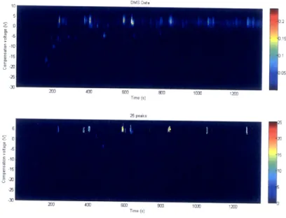
Figure 3-3: Number of more intense and wider peaks for 10 extractions for the de-pletion study. The threshold and n factor of the negative spectrum are 0.0078 and 0.0068.

used at extractions 1, 3, 4, 5, 6 and 7. Two measurements are used at extraction 2, 8, 9 and 10 due to abnormalities in the data. Therefore, the total number of files is 26. The first analysis involves the peak quantification of only the wider, more intense peaks in the positive and negative spectra. The threshold and n factor are 0.0080 and 0.0070. The second analysis is the quantification of any sized peaks; the threshold and n factor are lower values at 0.0078 and 0.0068. For most peaks, the negative slope is approximately 0.0010 more flat than the positive slope. The negative spectrum, Figure 3-3, demonstrates the peak quantification of larger peaks only and the algorithm identifies 14 large peaks. Another example of the positive spectrum is found in the Figure 3-4, which has a count of 25 large peaks.

The results of the peak numbers are presented in box and whisker plots. The red lines indicate the median, and the edges of the box indicate the lower and upper quartiles. Any remaining outer whiskers indicate the maximum and minimum values. The results of the larger peaks are found in Figure 3-5. For the larger peak counts, no

MKAQ n-t

.. 14

12

0 2 0.15 01 005 nime ts) 2 peaks 25 20 15 10 200 400 600 o00 100 1200 Time (s)

Figure 3-4: Number of large peaks for ten different extractions. The threshold and n factor of the positive spectrum are 0.008 and 0.007.

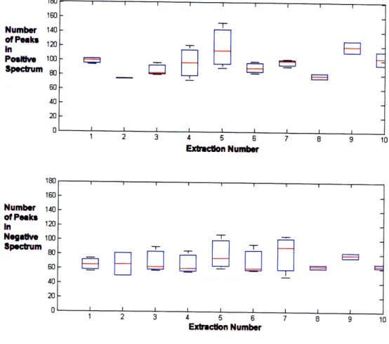
depletion effect of Tedlar bags appears to be present. After ten rounds of extractions which corresponds to 200 minutes (5 hours) and 10 injections per bag via the inlet ports, the breath sample from the Tedlar bag has not dropped in the number of peaks. The data still maintains approximately the same number of large peaks. Over the 26 files, the large peak count in the positive spectrum is 30 ± 5 peaks, and in the negative spectrum is 24 ± 8 peaks. Overall, more ions are detected in the positive spectrum of the DMS. The boxes are generally smaller for extractions at 2, 8, 9, and 10 since only 2 measurements are performed. No trends and no depletion are present, with respect to wider peaks.

The second analysis is a general count of the peaks (including small peaks) in these same 26 files. In order to count small and large peaks, the threshold and n factor are set at lower values, because the slopes of the smaller peaks rarely reach the previous threshold. For the positive spectrum, the threshold and n factor are 0.0066 and 0.0056, and for the negative spectrum, the values are 0.0050 and 0.0040 respectively. For the negative spectrum in Figure 3-6, the general peak count is 56. The peak quantification, shown in the bottom plot, reveals that small and large peaks are being selected. A positive spectrum example can be found in Figure 3-7, where

nmq ).f.

a

E 8

Number of Peaks in Posiive Spectrum Number of Peaks in Negative Spectrum 1 2 3 4 5 6 7 8 9 Extraction Number E E , I , I I 1 2 3 4 5 6 Extraction Number 7

Figure 3-5: Number of more intense and wider peaks for 10 study) are presented in box and whisker plots.

8 9 10

extractions (depletion

94 large peaks are identified.

The peak counts of small and large peaks are found in Figure 3-8. Over the 26 files, the general peak count in the positive spectrum is 96 ± 11 peaks, and in the negative spectrum is 70 ± 15 peaks. The positive spectrum found approximately 26 more peaks on average. It is noticed that the peak numbers in extraction #8 are lower and those in extraction #9 are higher. It is possible that small fluctuations occurred in the DMS, or perhaps the SPME fibers were not properly cleaned. From the quantitative analysis of large and general peaks, the conclusion is that there is no depletion effect of the Tedlar bags. After ten rounds of extractions, the data still

contains generally the same number of total peaks. If a breath diagnostic is developed, the Tedlar bag may be an effective way to store people's breaths over a long period

-T

OMS Data 10 25 -5 -10 15 -15 -20 05 -25 -30 56 peaks ~ 0

f

1.

!

Figure 3-6: Number of general peaks for ten rounds of extractions. The threshold and n factor of the positive spectrum are 0.0050 and 0.0040.

of time. It is a promising result that the Tedlar bags do not exhibit any depletion effects, and this investigation is performed by the peak quantification algorithm.

3.2

Peak Characterization

3.2.1

Definition of Peak Location, Width, and Intensity

After classification occurs and top features are selected, it is important to verify these key features. Often times, arbitrary pixels perform well for the classification, but no effective peak is present. The ideal situation is a peak in the diseased state and the absence of a peak in the non-diseased state. This peak in the diseased state can be a potential biomarker for TB. The peak characterization will check for legitimate peaks and characterize their locations, widths, and intensities.

A peak found in the DMS sensor data can be described by a peak location, width, and intensity. These definitions would be straight-forward if the peaks were sym-metrical. The peak locations would be the centers, and the widths could be defined

DMS Data

1

I,

Figure 3-7: Number of general (small and large) peaks for ten different extractions. The threshold and n factor of the positive spectrum are 0.0066 and 0.0056.

as the widths (in time and voltage) at half the intensity height. Most peaks are asymmetrical; thus the definition is more complicated. In this analysis method, the user initially defines a box around a specific peak. A local background subtraction algorithm is applied to remove any remaining background noise.

A peak position is reported as a point with two dimensions: a retention time and compensation voltage. The exact positions are determined by the marginal plots in both dimensions. The marginal profile in the x dimension is the summation of the

intensity values along the y axis for every x. The marginal profile in the y dimension is the total of the intensities along the x axis for every y. An example of these marginal profiles are displayed in Figure 3-9 for a peak from BSA.

The peak position in one direction is calculated as the weighted average in that direction. The marginal profile associates each point with a weight, wi which is mul-tiplied to each peak location, xi. After summing these weighted peak locations, the

overall value is normalized by the sum of the weights, W = wl + ...+ w,. Therefore,

the center of the peak, xo, is defined as the weighted average along the marginal profile of the peak:

E1 a 3

1 2 3 4 5 6 7 8 9 Number of Peaks in Spectrum Number of Peaks in Negative Spectrum 1 2 3 4 5 6 Exb.con Number 7 8 9 10

Figure 3-8: Number of general peaks for ten extractions presented in box and whisker plots.

0 = W (wi * xi) i=1

(3.5)

This weighted average accounts for bulkier sections of an asymmetrical peak. If a peak is biased to the right side, then these weighted values, wis, are larger and affect the peak location by biasing the location to the right. This peak location, or peak center, is determined in the time and compensation voltage dimension as (to, v,).

The general definition of a peak width, Ax, is twice the weighted standard

devi-ation, a: (Ax)2 = 2 (

)

I

I

--.-(a) Marginal Profile in Time (b) Marginal Profile in Vc

Figure 3-9: The peak position is indicated by an orange arrow and the peak width by an orange line. This y-axis is the marginal or weight value.

The standard deviation, a is half of the peak, so the peak's width is 2cr. The width is determined in the time and compensation voltage and reported as the peak half-width: (At, Av). The maximum intensity found in the boxed dimension corresponds to the height of the peak.

3.2.2

Reporting Values

An individual peak characterization is the determination of a peak's position, width, and maximum intensity. The Gaussian model and individual peaks can be displayed. The individual peak profiles provide information on the time marginals, Vc marginals, the 3D image, and the peak characterization values. Over multiple runs, the average and standard deviations of these quantities are determinable for different target peaks. The comparison of the data can show trends. Summary plots quickly illuminate any trends, and summary charts record precise values.

3.2.3

Results on Isoprene

The isoprene peak characterizations are displayed in the format of a summary plot. Isoprene is a standard used to build a library using the DMS sensor. Five peaks are selected in the data. The first peak is the isoprene peak whole elution time is at 205.8 s. The other four peaks are siloxanes whose elution times are 294.6 s, 468.0 s, 738.0

T 1 I I 1

NJ

s, and 787.8 s, as seen in Figure 3-10. 0 28 0 26 0.24 0.22 0.2 0.18 0.16 0 14 0 12 E 4 o 0 -6 Time (sec)

Figure 3-10: Zoomed-in DMS sensor data: 1 isoprene peak (205.8s) and 4 siloxane peaks

In one summary plot, a significant number of information can be gathered about a set of peaks. A summary plot has one x-axis and two y-axes; Figure 3-11 displays the x-axis of the time dimension. Five average peak locations are identified in the x-axis, which serves as the independent variable. The left y-axis is in time units and used to record the peak width averages in time, the standard deviations of the peak locations in time, and the standard deviations of the peak widths in time. It is helpful to observe the peak's width and observe how much the peak overall is deviating in peak location and in the peak width. Do the peaks stay overlapped over multiple runs. The right y-axis (green axis and a greeln line of data)is the detector intensity to measure the maximum intensity of the peak. Since each peak has one maximum intensity, this value is the same in figure 3-11 and 3-12.

It is quick to see the peak at 205.8 s that corresponds to the isoprene peak has the highest maximum intensity (0.33 DR) of the five peaks and located at (205.8 s, 2.6 V). The second highest intensity peak is a siloxane located at (787.8 s, 3.1 V) with an average maximum intensity of 0.21 DR. The isoprene half-width is (2.7 s, 1.34 V); the isoprene peak is the most narrow in the time dimension (see dark blue line) but the most wide in the Vc direction compared to the other five peaks. Its standard deviation in peak position is (0.4 s, 0.08 V) and its standard deviation in peak half-width is (0.35 s, 0.06 v). These standard deviations are particularly small in

the Vc direction compared to the large width of 2.6 V. The time-component standard deviations of the peak location and width make up approximately 1/6 of the overall peak half-width of 2.7 s.

This summary plot is useful for identifying the peaks with the higher maximum intensities or the peaks with the highest half-widths. Each peak can be analyzed individually to evaluate how much the peak location and peak width are fluctuating, with respect to the peak width. If the standard deviations are low, and the peak widths are large, then the peak is going to overlap well from one run to the other. However, if the peak width is small, and the standard deviations of the peak locations and/or peak widths are high, then the peak does not overlap at the same position very well. The summary plots displays a wide range of peak parameter characteristics in one graph. E 35 i 3 Co * 25 25 15

Peak Tmne Location (sec)

Figure 3-11: Summary plot of peak parameter characterization of isoprene and silox-anes for time dimension.

3.2.4

Results on Bacteria

The peak parameter characterizations are performed on the M. smegmatis data taken in February and April 2007. This section describes the summary charts, the intensity charts, and the individual peak profiles. The types of landmarks incorporated into this section are the siloxanes, which are introduced in Section 2.2.7.

Peak Vc Location (V)

Figure 3-12: Summary plot of peak parameter characterization anes for voltage dimension.

at .0 EO -2 U 32 .3 28 262 .24 22 .2 18

of isoprene and

silox-D05

Retention Time (s)

Figure 3-13: DMS sensor data taken from the lag phase of M. smegmatis in April 2007. (Color bar is the z-dimension of intensity in DR units). RIP line is absent.

April bacteria are the individual peak profiles and summary charts. In the DMS data, seen in Figure 3-13 six features are selected by a box figure, labeled, and characterized. These peaks consist of three siloxanes (peaks 1, 3, 4), one high-intensity peak (peak 2, it is called a HI peak if not identified as a siloxane; all siloxanes have high intensities), and two low-intensity (LI) peaks (peak 5, 6). The peaks are generically labeled 1-6. The high intensity peaks have slightly higher compensation voltages than the lower intensity peaks. It is in the area of the lower intensity peaks that the biological engineers suspect that possible biomarkers are located. These low intensity peaks are not visible at this scale but visible when zoomed in. Peak 6 was identified as a key feature by the classification as effective biomarker, but a closer look shows that it

015

0,1

may not be as stable and effective peak. The peak profiles and summary charts allow the assessment and screen for potentially good, robust VOC biomarkers and not just

pixels that performed arbitrarily well in the classification.

The average peak locations, widths, and maximum intensities of the six peaks in both data sets are described in three summary charts. The standard deviations enable the analysis of the general stability of the different peaks. Group 1 and 2 are the lag-phase M. smegmatis DMS data from February and April 2007 respectively.

Figure 3-14: Summary chart of peak parameter characterizations a high-intensity peak (peaks 1, 2).

Figure 3-15: Summary chart of

(peaks 3, 4).

for a siloxane and

peak parameter characterization for two siloxanes

Peak 1 (Siloxane) Peak 2 (High-Intensity) Group I Group 2 Group 1 Group 2 Peak Location 289.6s ± 1.0s 290.4s ± 2.1s 399.3s ± 0.8s 400.5s ± 2.16s

(time) o to

Peak Width, half 3.18s 0.22s 3.00s + 0.30s 2.41s ± 0.29s 2.38s 0.19s

(t ) A t At _-_

Peak Location 2.58V 0.11V 3.30V + 0.08V 2.48V ± 0.13V 3.25V ± .03V (Vc) V-'o ± V,

Peak Width, half 1.19V + 0.02V 1.20V + 0.01V 1.01V + 0.0" 1.00V 0.02V Peak Intensity - 0.247 ± .030 0.125 ± .015 0.151 ± .050 0.0'0 .006

(m=) max a1.

Box Center b, db (288s, 2.4) (289s, 2.8V) (398s,2.40V) (399s,3.00V) And Size (Atb Avb) (16s,6V) (16s 6V) (13s,5V) (13s,5V)

Peak 3 (Siloxae) Peak 4 (Siloxane)

Group 1 Group 2 Group 1 Group 2

Peak Location - 44".5s± .6s 44"7.'s 1.6s 33.0s ± 1.1s "35.4s ± 2.0s

(time) t_o ± a ro

Peak Width, half - 3.51s ± 0.60s 3.23s ± 0.41s 5.2"s ± 0..53s 4.20s + 0.58s

(time) t At

Peak Location - 1.7"V ± 0.14V 2.49V ± 0.05V 2.82V ± 0.24V 4.04V ± 0.03V (Vc) V a v

Peak Width, half 1.02V ± 0.03\ 1.03V + 0.02V 1.00V 0.04V 1.11V + 0.02V

(Vc) I

Peak Intensit - 0.103 + .018 0.061 + .004 0.150+ .030 0.062 ± .013 (Max) max u a,

Box Center (tb, d (448s, 2V) (289s, 2.8V) (398s, 2.40V) (398s, 2.40V)

Figure 3-16: Summary chart of peak parameter characterization for two low-intensity peaks (peaks 5, 6).

Some general characterizations that can be pointed out is that every average peak location is 1-2 seconds later in time; some fluctuation must have occurred to allow all the peaks to be shifted slightly in time. For group 1, the peak with the highest

intensity is the peak-i siloxane at 0.247 DR. For group 2, the highest intensity peaks are peak 2 and 4 with 0.150 DR. The intensity signal of peak 1 is strongest for group 1, but those of peak 2 and 4 are strongest for group 2. For the low-intensity peaks, peak 5 has an average lower intensity than peak 6 for group 1, but these two peaks have the same average intensity for group 2. The average maximum peak intensities for group 1 are higher than that in April for all six features from 2-7x more.

For group 1, the peak locations in time deviate slightly less than those in group 2, but the peak locations in Vc deviate slightly more. For group 1 and 2, the widest peak in time is peak 4 (siloxane) with a half-width of 5.27 s and 4.20 s respectively; and the widest peak in Vc is peak 1 (siloxane) with half-width of 1.19 V and 1.20 V. For these two peak characterizations, groups 1 and 2 match up. For the peak width standard deviations, group 1 has slightly larger standard deviations in the Vc dimension. There is no trend for the time dimension.

To get a sense of the peaks, let us look at the maximum intensities of four features over the 12 runs of group 2in Figure 3-17. The quantification of different peak

param-Peak 5 (Low-Intensit! Peak 6 (Low-Intensity)

Group 1 Group 2 Group 1 Group 2 Peak Location - 205.1s t 1.19t 206.1s .33s 311.5s 1 0.52. 313.5s ± 0.33s

(i c _{t + o}

Peak Width, half - 2.10 + ±0.51s 3.20s -0.23s 1.3s ± 0.26s 2.0s ± 0.14s Peak Locaton - -3.83 V 0.2V -4.3 - 0.09V -3.30V _ .0BV -2.34 0 .09V Peak Width, half 0.90'V 0.04V 1.05V 0.03V .68V ± 0.0"V .86V ± 0.04V

VC) Av ± cr

Peak Intensitr r 0.036 ± .012 0.010 ± .002 0.0-0 ± .016 0.010 ± .002

Box Center (tv -(20s, -5.8v (206s, -4.5 .312s, -3.2 ) (313s, -2.3V.

eters, such as maximum intensities, can now be tracked and reported with averages and standard deviations. No correlations occur, which indicate that all the peaks are not dropping or rising in a linear fashion from one run to another run.

Feature 1 Feature 5

Pmk Mxmk kdnMsiy OW 12 Runs HI Peak Pe Maxn, ktnW o 12 Run LI Peak

O.t124l1 -0.01S897 0 010 6.- 0.0207r 014 0135 .12 V 0O11

j0100

Peak Maawom Intmlly w.R 12 Rus HI Peak Peak Manmum ata noy 12 pa LI Peak

0 0on w- 0.0069 0 0006 -0 0014349

RnNwn* Run Numbt

Figure 3-17: Peak intensity of 4 peaks for group 2. No correlation is visually observed.

The following individual peak profiles will be of the lag phase of the bacteria from April (group 2). Twelve runs are available. The range of maximum peak intensity for the siloxanes and HI Peaks is 0.062 DR - 0.125 DR and for LI Peaks is 0.008 DR

- 0.012 DR. The individual peak profiles provide the peak parameter characteristics for one run. The future purpose would be that once a biomarker is identified, it can be described through the overall average and standard deviation values from the summary chart or plot, and it can be described through individual runs by the peak profile. These individual peak profiles summarize the peak's position, width, maximum intensity, box parameters and 3D shape for one run. The time and Vc marginal distributions within the specified box sizes are included and are normalized to 1. Figure 3-18 shows the individual peak profile of peak 1 (siloxane) of group 2. The maximum intensity of peak 1 (siloxane) is 0.140 DR. The location of peak is (292 s, 3.28 V). The half-width of the peak is (3.3 s, 1.20 V). The 3D peak profile is included to give the user a pictorial view of the peak.