An asymptotic result for the multi-stage weapon-target allocation problem

FEBRUARY 1990 LIDS-P-1945

An Asymptotic Result for the Multi-Stage Weapon-Target

Allocation Problem*

Patrick A Hosein

AT&T Bell Laboratories

Room 1C-422A, Crawfords Corner Road, Holmdel, NJ 07733

Michael Athans

Massachusetts Institute of Technology

Room 35-406, 77 Massachusetts Avenue, Cambridge, MA 02139

2 9th CDC Abstract

We consider a multi-stage version of the Weapon-Target Allocation problem. This problem models the following battle scenario. The offense launches a number of weapons (the targets) which are aimed at assets of the defense. These targets are assigned values by the defense. The defense has a number of (non-reusable) defensive weapons each of which can engage at most one target. The outcome of such an engagement is stochastic. In each stage of the engagement the defense observes the outcomes of the assignments made in the previous stage before assigning a subset of the remaining weapons in the present stage. The objective is to assign weapons to targets so as to minimize the total expected value of the targets which survive all stages.

In this paper we will assume that all targets have a value of unity and that the engagement of a target by a weapon depends only on the stage number. If we assume that the number of weapons used in each stage is linearly dependent on the number of targets then, we will show that, as the number of targets approaches infinity, the solution to this stochastic problem can be obtained by solving a related deterministic one.

1

Introduction

The Weapon-Target Allocation (WTA) problem is used to model the defense of assets in a military

conflict. The offense (the enemy) launches a number of offensive weapons which are aimed at

valuable assets of the defense. Since these weapons will be the targets of the defense's weapons,

henceforth we will call them targets. The defense has a number of defensive weapons with which

to engage these incoming targets. The engagement of a target by a weapon will be modeled as

a stochastic event. A probability, called a kill probability, will be assigned to each weapon-target

pair. This will be the probability that the weapon destroys the target if it is assigned to it. We

'This research was conducted at the MIT Laboratory for Information and Decision Systems with partial support provided by the Joint Directors of Laboratories under contract ONR/N00014-85-K-0782 and by the Office of Naval Research under contract ONR/N00014-84-K-0519.

will assume that the engagement of a weapon-target pair is independent of all other weapons and

targets. Note that a particular target may be engaged by more than one weapon (Salvo attacks).

Values are assigned to the incoming targets and the objective is to assign defensive weapons to these

targets so as to minimize the expected total value of the targets which survive after all engagements.

This corresponds to what is known as a weighted subtractive defense.l

In the multi-stage version, weapons are allocated in stages with the assumption that the

out-comes (i.e. survival or destruction of each target) of the weapon-target engagements of the previous

stage are observed (perfectly) before assignments for the present stage are made. We will assume

that each weapon can be used only once.

Some important properties of the multi-stage WTA problem are that it is (a) NP-Complete

(i.e. one must essentially resort to complete enumeration to find the optimal solution; see [7]),

(b) Discrete (fractional weapon assignments are not allowed), (c) Dynamic (the results of

previ-ous engagements are observed before making present assignments), (d) Nonlinear (the objective

function is convex), (e) Stochastic (weapon-target engagements are modeled as stochastic events)

and (f) Large-Scale (the number of weapons and targets is large, making enumeration techniques

impractical). These properties of the problem rule out any hope of obtaining efficient optimal

algorithms.

Several papers have been written on the single stage (or static) version of this problem. In

[3], denBroeder et al. consider the special static case in which the kill probability of a

weapon-target pair is independent of the weapon (i.e. a single class of weapons). They present an optimal

algorithm for solving this version of the problem. Kattar implemented this algorithm and presents

some numerical results in [6]. Matlin [8] and Eckler and Burr [4] give reviews of the material on

weapons allocation problems. However, in these studies, very little emphasis is given to the dynamic

allocation of weapons which is the main focus of our research. A major result, obtained by Lloyd

and Witsenhausen [7], is that the single stage version of problem is NP-Complete. What this means

is that the computation time of any optimal algorithm for the problem will grow exponentially with

the size of the problem. In conclusion, we have found that the open literature on the multi-stage

version of the WTA problem is scant. Furthermore, the literature which addresses this problem

1

The Weapon-Target allocation problem is but one of the many problems that are addressed in the field of Command and Control (C2) theory. The perspectives paper by Athans [1] presents some of the other basic problems.

contains few analytical results because of the difficulty of the problem.

2

Problem Definition

The multi-stage version of the WTA Problem consists of a number of time stages. The defense is allowed to observe the outcomes of all engagements of the previous time stage before assigning and commiting weapons for the present stage. This is called a "shoot-look-shoot-..." strategy since the defense is alternating between shooting its weapons and observing (looking) at the outcomes.

We assume that in the initial stage the defense chooses a subset of its weapons and assigns them to targets. These weapons are then committed simultaneously. In the second stage the outcomes (i.e. the survival or destruction of each engaged target) of all of the engagements of the weapons committed in the first stage are observed. Based on this observation, the defense chooses a subset of the remaining weapons and assigns them to the targets which survived the stage 1 engagements. In the third stage the outcomes of the engagements of the weapons committed in stage 2 are observed. Based on this observation, a subset of the remaining weapons is chosen and assigned to the set of surviving targets. This process is repeated for all time stages. In each stage the weapons are chosen and assigned with the objective of minimizing the total expected value of the surviving targets at the end of the final stage.

Note that in each stage the problem is re-solved based on the outcomes of the previous stage. This implies that in each stage one is interested in obtaining (a) the subset of weapons which are to be fired in that stage and (b) the optimal assignment of these weapons to targets. Note that in computing the optimal assignment for the present stage one must assume that in all subsequent stages an optimal assignment will be used. If this is not done then the expected cost for the problem could be improved by doing so. This is known as the Principle of Optimality in dynamic programming [2]. We will therefore implicitly assume that optimal assignments will be used in all subsequent stages.

Note that the only information required to compute the optimal assignments in a stage is the set of surviving targets, the set of remaining weapons and the number of stages left. All other information of previous stages is not relevant. Therefore at each stage the problem can be restated as one in which the present stage is the first stage of the restated problem. The initial set of targets for this problem is the set of surviving targets and the initial set of weapons is the set of remaining

weapons. In other words the problem to be solved at each stage has the same form as the statement

of the problem for stage 1. Therefore, although we will only consider the T-stage problem and solve

for the optimal assignments of the first stage, the same method can be used to solve for the optimal

assignments of the remaining stages.

In our notation we will index the parameters in each stage with the stage number. Therefore

for a T-stage problem the parameters in stage 1 will have an index of 1 while those of the final

stage will have an index of T. The notation to be used is as follows:

def

N

the number of targets (offense weapons),

M

the number of defense weapons,

T

the number of time stages,

def

V

the value of target i,

i = 1,2,...,N,

pij(t)d-

_{the kill probability of weapon j on target i in stage t,}

i = 1,2,...,N,

j = 1,2,...,M,

qij(t)-

1 - pij(t), the corresponding survival probability.

The decision variables will be denoted by:

_

1 if weapon j is assigned to target i in stage 1

zi=

0

The target state of the system in stage 2 will be defined as the set of targets which survive stage 1.

This state will be denoted by an N-dimensional binary vector iu E {0, 1}N and represented by

{_

|1

if target i survives stage 1,

u

0 if target i is destroyed in stage 1.

The weapon state of the system in stage 2 will be defined as the set of available weapons after stage

1. This state will be denoted by an M-dimensional binary vector

E {O, 1}M and represented by

_f 1 if weapon j was not used in stage 1,

0 if weapon j was used in stage 1.

Given a first stage assignment, {zij}, the target state at the start of the second stage is an

N-dimensional random vector. The probability that ui is 1 is the probability that target i survives

the first stage. The probability that ui is 0 is the probability that target i is destroyed in the first

stage. The distribution of the random variable ui is therefore given by:

Pr[ui

= k]

= k

II(1

pi(1))

_{ij + [1 - k] 1 -}

_p(1))

₍₁₎

for

k = 0,1,

i = 1,2,...,N.

Equation 1 will be called the target state evolution of the system.

The weapon state also evolves with time. This evolution is deterministic and depends on the assignments made in the first stage. The evolution is given by:

N

wj -

= 1,2,...,M.

j, j

(2)

i=l

This simply says that weapon j is available in the second stage if and only if it is not used in the first stage. Equation 2 will be called the weapon state evolution of the system.

We will let F2(i, tw) denote the optimal cost of a T - 1 stage problem with initial target state

i

T - 2-stage problems, etc. Eventually the (T - (T - 1) or single stage problem will be defined in

terms of optimal costs for O-stage problems. The optimal cost of a O-stage problem will be defined as:

N

Fj+(1 (w) =

ZE

i=l

In other words, the cost is simply the total value of the targets which survived the final stage. Problem 2.1 The Multi-Stage Weapon-Target Allocation problem (MWTA) can now be stated as:

min F, =

Pr[tu = ]F;(w, 5)

with wtj=l-

xij.

The objective function is the sum, over all possible stage 2 target states, of the probability of

occurrence of that state times the optimal cost given that state. The probability distribution of the target state was given in 1. Note that the distribution of the stage 2 target state and the stage 2 weapon state both depend on the first stage assignment. The first constraint restricts each weapon to be assigned at most once in the first stage. The second constraint is due to the weapon state evolution.

This problem is difficult both analytically and computationally. This can be illustrated by at-tempting to use a straightforward dynamic programming approach to the problem. Let us consider a two stage problem. The number of possible weapon subsets that can be chosen in the first stage is 2M. If ml weapons are used in stage 1 the number of possible assignments that must be checked

is Nm'. If N of the N targets are engaged in the first stage the number of possible outcomes is 2N.

If N of the N targets survive stage 1 and m2 weapons are available in stage 2 then the number

of assignments that must be checked to obtain the optimal cost for this outcome is rNm2. These numbers show the enormous number of computations that will be required if a straightforward dynamic programming approach is used. Note that to simply evaluate the expected value of a first stage assignment requires a tremendous computational effort.

3

The Single-Stage Problem

In this section we will present the special case of the problem in which there is only one stage. This problem has been well studied in the literature. It has been shown by Lloyd and Witsenhausen [7] to be NP-Complete in general. Therefore, only sub-optimal algorithms have been proposed for its solution.

We will see in the next subsection that if we assume that the kill probabilities do not depend on the weapons (i.e. we have a single class of weapons) then the resulting problem can be solved by a polynomial time algorithm. This implies that the basic difficulty of the problem stems from the fact that there are multiple types of weapons. The problem is also difficult because of the non-linearity of the objective function.

3.1 Special Cases of the Single-Stage Problem

Two optimal algorithms exist for solving this problem under the additional assumption that the kill probabilities are independent of the weapons, i.e. Pij = Pi. This assumption is valid if the defense has a single type of weapon and all weapons are located in the same area so that the geometry and time of intercept is the same for all. denBroeder et al. [3] proposed the first algorithm for solving this special case of the problem. Their's is essentially a greedy algorithm in which weapons are assigned sequentially to the target for which the corresponding decrease in the cost is maximum. This algorithm is usually referred to as a Maximum Marginal Return algorithm. The second

algorithm for solving the problem is a Local Search algorithm. The algorithm starts with any feasible solution and searches locally for a better solution until the optimal one is found. Proof of

optimality of this algorithm can be found in [5].

In the previous paragraph we had assumed that the kill probability is independent of the weapons. In this paragraph we will assume that for each weapon-target pair the weapon can either be assigned to the target or it cannot be assigned to the target (i.e. each weapon can only reach some of the targets). If it can be assigned to the target then we will assume that the kill probability of the pair is only dependent on the target. In other words we are assuming that the kill probability of a weapon-target pair is either 0 or some target dependent value pi (i.e Pij E {0, Pi}). This problem can be re-formulated as a Linear Minimum Cost Network Flow problem. Any algorithm for solving such problems can then be used to find the optimal solution.

Another special case is that in which each target can be assigned at most one weapon. This problem can be re-formulated as a Transportation problem. Any algorithm for solving Transporta-tion problems can then be used to find the optimal soluTransporta-tion.

4

Unit Valued Targets and Stage Dependent Kill Probabilities

In this section we will study the effect of stage dependent kill probabilities p(t) on the optimal assignment. We will assume that the targets all have a value of unity and that the kill probabilities

p(t) are independent of the weapons and the targets. We were not able to obtain an analytical

solution to this problem even for the case of two targets. However, we were able to obtain results for the limiting case, as the number of targets goes to infinity. We will first present some properties of the optimal solution.

Theorem 4.1 Consider the Multi-Stage WTA problem in which there are T stages, N unit-valued targets, stage dependent kill probabilities p(t), and M weapons. The optimal strategy has the prop-erty that the weapons to be used at each stage are spread as evenly as possible among the surviving targets.

The above result simplifies the problem to be solved since we can use the number of weapons

to be used at each stage, (denoted by mt), as the decision variable and optimize over this variable.

Given the optimal values of mt, the optimal assignment can then be obtained by spreading these

weapons evenly among the targets. In the case of T = 2 the resulting problem is a one dimensional

optimization problem since ml + m

= M. Intutively we would expect the expected cost to be a

unimodal function with respect to the number of weapons used in stage 1. However, this is not the

case as we see in the following two-stage example.

0 LL _

0I

0 2 4 6 8 10 12 14

ml

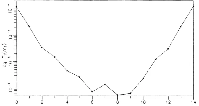
Figure 1: A two-stage example in which the expected cost as a function of the number of first stage

weapons, Fl(ml), has multiple local minima.

Let us choose ml, the number of first stage weapons, as the independent variable. We will

write the expected value if ml weapons are used in stage 1 and M - ml weapons are used in

stage 2 by Fi(ml). The optimal solution can then be obtained by minimizing Fi(ml) over the

set {0,1,..., M}. If Fi(ml) was a unimodal function of ml then this minimization could be done

efficiently by using a local search algorithm. Unfortunately, this is not the case as can be seen in the

following example. Consider the problem in which T = 2, M = 14, N = 3 and p(l) = p(2) = 0.9.

In Figure 1 we have plotted logFl(ml

versus ml. Here we find an example in which there are

multiple minima. This implies that the problem is difficult since one essentially has to do a global

search to obtain the global minimum.

Note that we used a log scale because the variations near the global minimum are so small that,

with a linear scale, the function "appears" to have a single minimum. This suggests that for all

practical purposes any of the local minima will suffice. A local minimum can easily be obtained

by a local search algorithm (i.e. repeatedly increase or decrease ml, if doing so decreases the cost,

until any change in ml results in an increase in the cost.

4.1

The Limit of an Infinite Number of Targets

In this subsection we will consider what happens for very large numbers of unit-valued targets. We

will keep the ratio of weapons to targets fixed and solve the problem in the limit as the number

of targets goes to infinity. We will find that, in the limit, the problem can be considered as a

deterministic one in which the number of targets in a stage is the expected number of targets which

survive the previous stage.

Let us introduce the variable nt

This is the number of weapons reserved for stage t per

initial number of targets. We will also define the vector

Rt for 1

t < T by

Not be optimal for the problem. We will address the question ofT

Note that the values of Kt may not be optimal for the problem. We will address the question of

finding optimal values for st in the following subsection. By theorem 4.1 we know that the weapons

to be used in each stage should be spread evenly among the surviving targets. The expected cost

of the T-stage problem with N targets and in which mt = rctN weapons are used in stage t will be

denoted by Fl(N,

il).

Let a denote the expected fraction, of the initial number of targets, which

survive stage 1 i.e.

a = [1-(K1 -lK1J)p((1 - p(l))L-"J.

(4)

Note that a is independent of N. Consider the case of the single-stage problem (i.e. T = 1). We

have

F(N,:)

_

a = [1-(k -

[L

rJ)p(l)](l- p(l))L

1J

N

Taking the limit as N goes to infinity on both sides we get

lim Fi(N, l) = [1 (1 -l - L )p(2)](1 -p(2))L 'J = a. (5)

N-.oo N

In other words, for the single-stage problem, if the weapon to target ratio is kept fixed then the

expected fraction of targets which survive is the same for all values of N. This will also be the

value in the limit as the number of targets goes to infinity. We will now show how the limit of this

ratio can be obtained for more than one stages. The limit for the T-stage problem will be obtained

in terms of the limit for the T - 1 stage problem, etc. Since the limit for the case T = 1 is well

defined then the limit for the two-stage problem is well defined etc. The T-stage limit is therefore

well defined. The main result will now be presented.

Theorem 4.2 Consider the T-stage problem with N unit valued targets, M = KN weapons and

stage dependent kill probabilities p(t). Assume that the number of weapons to be used in stage t is

given by mt = KtN, where rt E [0, ;] is a fized constant which may be different for each stage. We

then have that

lim F(N

lim F2(N,2/(6)

N-oo N N--oo N

where a is given by equation 4.

Proof: Let N2 represent the number of targets which survive stage 1. N2 is a random variable. If

nK is an integer then it is a binomial random variable; otherwise, its distribution can be obtained by the convolution of two binomial distributions. The mean and variance of this distribution is given by:

E[N2] - N2 = aN,

Var[N2] = a2 = /3N,

where

P = q(l)Lt1J[(1 - (r1- - LKJ))(1 - q()LK1J) + (Ki - LKjj)q(1)(1 - q(1)L']J+l)] Note that

/3

F1(N,riv) = Pr(1N2- N21 > piN)E[F2(N2,K2)[IN2 - N21 > AN)]

+ Pr(lN2 -

N2

N2

pN)].

By Chebyshev's Inequality we know that

Pr(IN2 - R21 < /N) > 1 (- N)2 1- (8) -- N)1 A2N

Since F2(N2, Fi2) is a monotonically increasing function of N2 then

and

E[F2(N2, 2)11IIN2 - 2

1

IAN]

and also

E[F

(N

,9

)IIN

N

> tN]

<

Using 8 9, 10 and 11 in 7 we obtain

(1-

L )F2(VN2 -

N, 2) < Fl(N,.)

< P2 [F2(N, R2)] + F2(N2 + N,

K2)

(12)

p2N 2N

Dividing by N and taking the limit as N goes to infinity we obtain

lim F2(N 2-IN, 2) < lim Fi(N,1) < lim F2(2

+/ N,

N-.oo N - N-coo N - N-.oo

N

Using the fact that -N

= aN and taking /z arbitrarily close to 0 we obtain

lim

(a N,

Using a change of variables we finally obtain

lim

(N,)

a lim

This completes the proof. ·

Note that the theorem gives the limit of the T-stage problem in terms of the limit for a (T -

1)-stage problem. The latter can be expressed in terms of the limit of a (T - 2)-1)-stage problem etc.

The limit for the case T = 1 is given in equation 5. This limit provides us with a lower bound for

finite values of N. This result is given in the next theorem.

Theorem 4.3 Consider the T-stage problem with N unit valued targets, M = r;N weapons and

stage dependent kill probabilities p(t). Assume that the number of weapons to be used in stage t is

given by mt =

where

E [0,K] is a fixed constant which may be different for each stage. We

then have that

F1(N,

K1) > N lim

l

(13)

Proof: Let k be any positive integer. Consider the problem with kN targets and in which mt = ksctN

weapons are used in stage t. Let Fl(kN, il) denote the optimal cost for this problem. A sub-optimal solution for this problem is the following. Split the problem into k subproblems. Each of these subproblems has N targets and uses mt = r;tN weapons in each stage. The optimal cost for the problem under this restriction is given by kFl(N, il). Since this solution is suboptimal we have:

Fl (kN, i1) < kFl (N, ~ij).

Dividing both sides by kN and taking the limit as k goes to infinity we have F (N,1) > lim Fl(kN,Il)= lim F(,* 1

)

N - .-oo kN -..oo ST

The result 13 now follows. ·

Theorem 4.3 provides us with a lower bound on the optimal cost for the problem with finite values of N. Theorem 4.2 is more easily understood if we look at some examples.

Example 1

Suppose that K = 2, K1 = 0.5, n2 = 1.5 and p = 0.6. In other words the defense has 2N weapons,

N/2 weapons are used in stage 1 and the remainder are used in stage 2. The expected fraction of

targets which survive stage 1 is given by

a

-[(1

Therefore the expected value in stage 2 given that the expected number of targets survive stage 1 is given by:

F2(a, ;K2) = F2(0.7, 1.5) = [(1 - p)3 + 6(1 - p)2]/10 = 0.1024.

Note that we had to scale the number of weapons and the number of targets by a factor of 10 so that there are an integral number of each. If we now use the theorem we obtain:

lim F1(N, [.5, 1.5]) 0.1024.

N-.oo N

In words this says the following. For very large N, if 25% of the weapons are used in stage 1 then approximately 10% of the targets will survive both stages. For comparison, if a single stage

strategy is used then 16% of the targets will survive. If we consider the case of two targets, N = 2,

then 13.12% of the targets will survive both stages.

Example 2

Consider the 3 stage problem with rK

rK

and p

0.5. In the limit the expected

fraction of targets which survive stage 1 is

The expected fraction which survive stage 2 is

and

the expected fraction which survives stage 3 is 21-r. Therefore,

lir

F

(N, [1,1,1])

2_.

Let us now consider a case with stage dependent kill probabilities.

Example 3

Suppose that el = [1.5,1,.5] and that p(l) = .6,p(2) = .5,p(3) = .4. The expected fraction of

targets which survive stage 1 is given by

a = 0.5[(1 - p(l)) + (1 - p(l))

] = 0.28.

The expected fraction which survives stage 2 is the solution to a static problem with 0.28 targets

and 1 weapon. To find the limit for this problem we find the cost for the case of 7 targets and 25

weapons (i.e. multiply by 25) and divide the cost by 25. We obtain

a = [4(1 - p(1)) 4) + 3(1 - p(1))3]/25 = 0.025.

The expected fraction which survives the final stage is the solution to a static problem with 0.025

targets and .5 weapons. Multiplying the parameters by 40 etc. we obtain

a =

(1

p(2))2°/40

9.1

Therefore in the limit as the number of targets goes to infinity, the expected fraction of the initial

number of targets which survives all stages is 9.1 x 10

Theorem 4.2 is important because it allows us to compute approximate costs for the case of

large N. This approximation is typically good for values of N greater than 100. Theorem 4.3 says

that this limit provides a lower bound on the cost for finite values of N.

In words theorem 4.2 says the following. Let us suppose that the number of weapons reserved for a stage is linearly dependent on the initial number of targets N. Therefore, as we increase the number of targets, the number of weapons in each stage will increase at the same rate. As we increase the number of targets, the expected number of targets which survive the final stage will also increase. Let us instead consider the ratio of the expected number of surviving targets and the initial number of targets. The theorem says that we can compute this ratio in the limit of an infinite number of targets N by solving a related deterministic problem. This deterministic problem is obtained as follows. Let us suppose that at each stage the number of surviving targets is equal to the ezpected number of surviving targets. Pick the initial number of targets N so that the expected number of surviving targets at each stage is integral. Using this value of N we evaluate the expected surviving number of targets at the end of the final stage of the deterministic problem in which, at each stage the expected number of surviving targets survive the previous stage. The ratio of the expected number of surviving targets for this problem and the initial number of targets

N is the same as the ratio, in the limit as N goes to infinity, of the expected number of surviving

targets and the initial number of targets. Note that the former ratio is obtained by solving a deterministic problem while the latter ratio must be obtained by solving a stochastic problem for an infinite number of targets. This limit provides a lower bound for the ratio for finite values of N. Furthermore, it provides an approximate answer for large values of N.

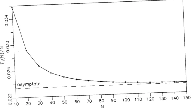
Let us take the following example. Consider the problem of two stages T = 2 with M = 2N weapons. N weapons are used in each of the stages (i.e. K = [1, 1]). We computed the exact value

of the ratio F. (N,) for N = 10, 20,..., 150, and also in the limit as N goes to infinity. In figure 2 we have plotted this ratio for finite values of N as well as the ratio in the limit of infinite N. In this case we used a second stage kill probability of p(2) = 0.7 and a first stage kill probability of

p(l) = 0.6. Additional examples of this kind may be found in [5].

4.2

Optimal Number of First-Stage Weapons for a Two-Stage problem with a

Large Number of Targets

Note that, in the discussion in the previous subsection, the number of weapons to be used in each stage was fixed. In this section we will find optimal values for g as N goes to infinity. This will give us a good approximation to the optimal solution for large values of N.

r) C? Z O

asymptote

Figure 2: The ratio of the expected two-stage cost and the initial number

of targets N vs. N for

p(1) = 0.6,p(2) = 0.7; N weapons are used in each stage.

We will only consider the two-stage case, T = 2. The optimization could

also be attempted for

T > 2, but it is doubtful whether one can find an analytical solution

for such cases. For the case

T = 2 we know that K2 = r - rK since all remaining weapons are used in the second stage. We

therefore have a one dimensional optimization problem. We will let K1 be the free variable. The optimization problem can be stated as:

min F2(a,K - K1) (14) subject to Kl E [0, ] where a = [1 - (l- [KlJ)p(1)](l - P(1)) '_J '

The function F2(a, r;2) is given by:

F2(a, r2) = [a - p(

2_{)(;K2 -}

_aL[-

This function is difficult to minimize. However, if the integrality constraint

is relaxed, then the

expected cost is given by aq(2) a. Since this is a lower bound for the

non-relaxed problem, then

F2(a, c2) > aq(2)?.

This states that the solution obtained by allowing fractional assignments in the second stage is a lower bound to the solution in which only integral assignments are allowed. Note that if a is a non-negative integer then equality holds in expression 15. Therefore, if the solution to the problem using the lower bound as the objective function is a multiple of a then it is optimal for the true problem.

The optimization problem using the lower bound in 15 as the objective function can be stated as:

min aq(2) (16)

subject to 1cl E [0, n] where

a = [1 - (K₁ -

KliJ)p(1)](1

.

Let us first consider the case I = 1. The solution is simply that all weapons should be assigned in the stage with the higher kill probability. Therefore,

t; = 0 for p(1) < p(2) (17)

;=l1 for p(l) > p(2) (18)

Let us now consider the case in which K = 2, i.e. a 2:1 weapon to target ratio. Using straight-forward calculus one can show that the optimal values of K1 are given by

r.-0 for 2p(l)-1 1(19) p(l) - log(1 - p(2)) K* =1 for 2p(1)-1

1

optimal for problem 14. Otherwise Cl is approximately optimal.

In the plot in figure 3 the vertical axis represents the kill probability in stage 1 while the horizontal axis represents the kill probability in stage 2. In each region we have indicated the optimal value of ml, the number of weapons allocated in the first stage (recall that ml = rKN) for

0 ml=N / 6 \ N<-1,<2N ml=N m,=2N (0

o

'

l

l

l

l

l=0

Figure 3: Optimal number of first-stage weapons, ml, for various kill probabilities with M = 2N

weapons, in the limit of an infinite number of targets, N.

the kill probabilities in that region. For example, consider the case p(l) = 0.8. If 0 < p(2) < 0.15 then it is optimal to use all weapons in stage 1. If 0.15 < p(2) < 0.55 then the optimal number of weapons to be used in stage 1 lies between N and 2N. If p(2) > 0.55 then it is optimal to use half of the weapons in stage 1.

Note that for 0.6 < p(l) < 0.9 and 0.6 < p(2) < 0.9 it is optimal to use half of the weapons in stage 1. This implies that for the problems of interest to us (i.e. large-scale problems with kill probabilities greater than 0.6) it is optimal to use half of the weapons in stage 1, even if the kill probabilities are different in each stage. This insensitivity of the optimal strategy to the kill probabilities is very interesting. We should stress that this result is valid for large numbers of unit-valued targets and weapons

5

Conclusions

In this paper we considered a multi-stage version of the Weapon-Target Allocation problem. Under suitable assumptions we have shown that, as the number of targets approaches infinity, the problem can be treated as a deterministic one in which the number of targets which survive a stage equals its expected value. This result can be used to gain insight into Large-Scale versions of the more

general problem and can also be used to provide lower bounds on the optimal cost for problems with a finite number of targets.

References

[1] Athans M., "Command and Control (C2) theory: A Challenge to Control Science," IEEE

Transactions on Automatic Control, vol. AC-32, pp. 286-293, April 1987.

[2] Bertsekas, D. P., Dynamic Programming. New Jersey: Prentice Hall Inc. 1987.

[3] denBroeder, G. G., Ellison, R. E., and Emerling, L., "On Optimum Target Assignments,"

Operations Research, vol. 7, pp. 322-326, 1959.

[4] Eckler, A. R., and Burr, S. A., Mathematical Models of Target Coverage and Missile Allocation. Alexandria, Va.: Military Operations Research Society, 1972.

[5] Hosein, P. A., A Class of Dynamic Nonlinear Resource Allocation Problems. PhD thesis, Mas-sachusetts Institute of Technology, Cambridge, MA., Sept. 1989.

[6] Kattar, J. D., "A Solution of the Multi-Weapon, Multi-Target Assignment Problem," Working Paper 26957, MITRE, Feb. 1986.

[7] Lloyd, S. P, and Witsenhausen, H. S., "Weapons Allocation is NP-Complete," in Proceedings

of the 1986 Summer Conference on Simulation, (Reno, Nevada), July 1986.

[8] Matlin, S. M., "A Review of the Literature on the Missile-Allocation Problem," Operations