HAL Id: tel-01416242
https://hal.archives-ouvertes.fr/tel-01416242
Submitted on 19 Apr 2017
HAL is a multi-disciplinary open access archive for the deposit and dissemination of sci-entific research documents, whether they are pub-lished or not. The documents may come from teaching and research institutions in France or abroad, or from public or private research centers.
L’archive ouverte pluridisciplinaire HAL, est destinée au dépôt et à la diffusion de documents scientifiques de niveau recherche, publiés ou non, émanant des établissements d’enseignement et de recherche français ou étrangers, des laboratoires publics ou privés.
Contribution à la Résolution Algébrique et Applications
en Cryptologie
Guénaël Renault
To cite this version:
Guénaël Renault. Contribution à la Résolution Algébrique et Applications en Cryptologie. Calcul formel [cs.SC]. UPMC - Paris 6 Sorbonne Universités, 2016. �tel-01416242�
U
NIVERSITÉ
P
IERRE ET
M
ARIE
C
URIE
HABILITATION À DIRIGER DES
RECHERCHES
Spécialité
Informatique
Contribution à la Résolution Algébrique et
Applications en Cryptologie
Présentée et soutenue publiquement par
Guénaël Renault
le
jeudi 8 décembre 2016
après avis des
rapporteurs
M. Pierre-Alain FOUQUE Professeur, IUF et Université Rennes 1
M. Éric SCHOST Associate Professor, University of Waterloo
M. Émmanuel THOMÉ Directeur de Recherche, INRIA Lorraine
devant le
jury composé de
M. Jean-Charles FAUGÈRE Directeur de Recherche, INRIA Paris
M. Pierre-Alain FOUQUE Professeur, IUF et Université Rennes 1
M. Emmanuel PROUFF Expert (HDR), Safran Identity and Security
M. Mohab SAFEYELDIN Professeur, IUF et UPMC
M. Éric SCHOST Associate Professor, University of Waterloo
Table des matières
1 Introduction et Synthèse 3 1.1 Introduction . . . 3 1.2 Problèmes galoisiens . . . 5 1.3 Problèmes diophantiens . . . 7 1.4 Problèmes PoSSo . . . 91.5 Liste des publications depuis 2006 . . . 13
2 Contribution to Effective Galois Theory 17 2.1 Introduction . . . 17
2.2 Splitting field computation . . . 18
2.2.1 Computation schemes . . . 19
2.3 Radical representation of roots and applications . . . 24
2.3.1 Rational and deterministic encoding from solvable polynomials . . . 25
2.3.2 De Moivre’s polynomials . . . 25
3 Contribution to Coppersmith’s Algorithm 29 3.1 Introduction . . . 29
3.2 Coppersmith’s method for finding small roots . . . 31
3.3 Application to combined attack on RSA-CRT . . . 33
3.4 Rounding and chaining for Coppersmith’s algorithm . . . 34
4 Contribution to Polynomial System Solving 37 4.1 Introduction . . . 37
4.2 Point decomposition problem and polynomial system solving . . . 38
4.2.1 Problematic . . . 38
4.2.2 On using symmetries . . . 39
4.2.3 From geometric symmetries to algebraic structures . . . 40
4.2.4 Size estimation . . . 42
4.3 Solving polynomial systems with symmetries . . . 43
4.4 Gain of efficiency in the resolution of the PDP with 2-torsion action . . . 47
4.5 Symmetries in characteristic 2 . . . 48
C
HAPITRE
1
Introduction et Synthèse
1.1 Introduction
Afin de positionner au mieux les résultats qui seront présentés dans la suite de ce document, il est important de commencer par en définir le titre.
Résolution algébrique. Lagrange, dans [94], est l’un des premiers mathématiciens à donner une définition de cette expression qui nous semble la plus adaptée. En effet, dans cet ouvrage il se propose d’étudier la résolution des équations polynomiales sous forme de radicaux. Plutôt que d’essayer de produire de nouvelles formules pour la résolution d’équation particulières, comme c’était le cas jusqu’à présent, il essaie de faire une synthèse de toutes les méthodes existantes afin d’en extraire une méthode algébrique générale. Même s’il a conscience que son objectif principal ne sera pas atteint, il montre clairement qu’il a compris l’essentiel de la démarche algorithmique permettant de décider la résolubilité par radicaux de ces équations (voir l’extrait ci-après issu de l’ouvrage [94] datant de 1770). Cette démarche algorithmique où l’ensemble des données manipulées restent symboliques et les outils employés sont essentiellement algébriques définit la résolution algébrique. Bien sûr, cette démarche fait aujourd’hui partie du calcul formel et peut être appliquée à d’autres problèmes que ceux de la résolution sous forme de radicaux, comme
4 CHAPITRE1. Introduction et Synthèse
par exemple : les problèmes diophantiens ou la résolution des systèmes polynomiaux.
Un autre point important mis en avant par Lagrange est l’utilisation de structures intrinsèques à ces équations. C’est ce qu’il appelle combinaison et que nous appelons aujourd’hui action du groupe de Galois. Ainsi, il décrit ici un principe général de résolution où il est nécessaire d’utiliser des structures particulières au problème pour y répondre au mieux.
Depuis, nombre de mathématiciens, d’informaticiens suivent ce principe. L’objectif principal étant de développer des algorithmes efficaces en considérant toutes les particularités du pro-blème donné plutôt que d’appliquer des stratégies trop génériques. Pour le propro-blème étudié par Lagrange, en toute généralité il n’y a pas de solution possible, alors que si l’on considère la structure de groupe associée, on peut, dans les bons cas, résoudre le problème efficacement. Ce qui fait toute la puissance de cette approche en fait aussi sa difficulté, ne serait-ce qu’identifier les structures qui permettent de résoudre plus efficacement est parfois un problème en soi. En fonction du contexte, ces structures peuvent provenir de la définition même du problème, de sa modélisation, des quantités prenant part au calcul ou encore de la nature de la sortie. Les travaux présentés dans la suite de ce document suivent tous cet axe de recherche et ont pour certains des applications en cryptologie.
Applications en Cryptologie. La sécurité des systèmes cryptographiques asymétriques (e.g. ceux permettant l’échange à distance de clés secrètes) reposent généralement sur des problèmes algébriques. En particulier, le niveau de sécurité se mesure en fonction des coûts en temps de calcul des meilleurs algorithmes connus permettant de résoudre ces problèmes. Ainsi, ce do-maine de l’informatique fournit une panoplie de problèmes qui sont souvent très structurés et donc représente un creuset pour le développement de nouveaux algorithmes ad hoc de résolution algébrique.
Bien que tous les résultats présentés ci-après suivent ce même axe de recherche, ils peuvent se différencier à travers les problématiques traitées. Ainsi ils peuvent être regroupés selon trois familles de problèmes généraux :
— Problèmes galoisiens : c’est la représentation formelle des racines d’un polynôme en une variable qui nous intéresse ici, pouvoir les manipuler symboliquement ainsi que les actions galoisiennes qui leur correspondent.
La structure naturelle que nous avons utilisée pour résoudre efficacement ces problèmes est l’action du groupe de Galois sur les racines du polynôme. Nous détaillons les résultats obtenus dans la section 1.2.
— Problèmes diophantiens : On s’intéressera plus particulièrement au calcul de petites racines entières d’équations diophantiennes.
Ici c’est la nature même des solutions cherchées qui guide le processus de résolution. En particulier, nous nous sommes intéressés à l’algorithme de Coppersmith qui résout ce problème en temps polynomial lorsque ces racines sont suffisamment petites. La section 1.3 présente les résultats obtenus.
— Problèmes PoSSo : PoSSo pour Polynomial System Solving, ainsi on s’intéresse ici à la résolution de systèmes polynomiaux ayant un nombre fini de solutions et à leurs applica-tions en cryptologie.
1.2. Problèmes galoisiens 5 Dans ce cadre, ce sont des problèmes de cryptanalyse qui ont motivé nos recherches. En particulier, nous nous sommes intéressés à l’utilisation des symétries apparaissant lors de la résolution du DLP sur certaines courbes elliptiques. Les résultats sont détaillés dans la section 1.4.
Dans la suite de ce chapitre, une synthèse des résultats obtenus selon ces trois familles de pro-blèmes est présentée. Ces résultats ont tous été obtenus après 2006 et ne font pas partie de ceux obtenus durant ma thèse.
1.2 Problèmes galoisiens
Une première partie des travaux relevant de la théorie de Galois font suite à ceux réalisés au cours de ma thèse. Les travaux présentés dans cette section ont été obtenus avec la collabora-tion de Jean-Gabriel Kammerer, Masanari Kida, Reynald Lercier, Sébastien Orange et Kazuhiro Yokoyama.
Ici on s’intéresse à la représentation formelle des racines d’un polynôme f en une variable. Plus exactement ce problème général est défini comme suit.
Problème 1. Soit f un polynôme en une variable de degré n > 0 et à coefficients dans un corps K. Donner un algorithme permettant d’exprimer les racines de f de manière à pouvoir les manipuler formellement.
Une première réponse à ce problème s’inscrit directement dans les travaux de Lagrange, Galois, Abel et Jordan (voir [125] pour plus de détails) portant sur la mise en place d’une méthode générale permettant la résolution sous forme de radicaux d’équations polynomiales. Nous savons aujourd’hui que cette approche ne peut donner une solution en général. Seules les équations de groupes de Galois G résoluble ont des solutions exprimables de la sorte. Du point de vue de la complexité, on sait d’après Landau et Miller [98] que dans ce cas le calcul d’une telle représentation peut se faire en temps polynomial.
De manière générale, pour représenter les racines de f formellement, nous devons passer par la représentation de son corps de décomposition. Ceci peut se faire sous la forme d’un quotient K[x1, . . . , xn]/M où M est appelé idéal des relations algébriques des racines de f. Cet idéal est défini comme le noyau du morphisme de K[x1, . . . , xn]dans la clôture algébrique ¯K qui à xi fait correspondre la racine ↵i(on peut noter que cette définition dépend de l’ordonnancement des racines). Ainsi, dès que l’on a une base de Gröbner de l’idéal M, il devient possible de calculer formellement avec les images des xidans ce quotient, chacune représentant une racine de f.
Le calcul d’une base de Gröbner de M peut être réalisé à l’aide d’un algorithme simple pro-cédant par factorisations successives dans une tour d’extensions construites à partir des racines de f. D’après [97] cet algorithme a une complexité polynomiale en la taille |G| du groupe de Galois de f et la taille de f (norme L2 des coefficients de f). Cette complexité est la même lorsque l’on souhaite calculer une représentation symétrique du groupe de Galois G.
Nos travaux dans ce domaine s’intéressent à un autre algorithme que celui-ci pour calculer la base de Gröbner de M. Ils s’appuient sur une méthode décrite par Yokoyama dans [144] et
6 CHAPITRE1. Introduction et Synthèse
étendue dans [131] en collaboration avec ce dernier. Cette méthode repose sur l’interpolation des polynômes prenant part à la base de Gröbner de M et utilise l’action du groupe de Galois G sur des approximations p-adiques des racines de f pour réaliser ce calcul.
Les résultats principaux que nous avons obtenus dans la suite de ces travaux ont permis d’exploiter au mieux cette action de groupe lors du calcul de la base de Gröbner de M. Le gain en efficacité pratique atteint un facteur de l’ordre de plusieurs centaines. Concernant la complexité asymptotique, nous montrons que le coût combinatoire des calculs nécessaires à l’utilisation de cet action reste bornée par |G| et donc ne modifie pas la complexité générale. Dans la suite nous détaillons plus précisément chacun des résultats obtenus dans cet axe de recherche.
Dans la continuité de [131], nous montrons dans [132] comment adapter l’approche modu-laire à une approche multi-modumodu-laire. Le problème se posant ici est que les approximations des racines modulo différents premiers ne coïncident pas forcément. Nous proposons une méthode de reconnaissance des bonnes associations de ces différentes images en utilisant des invariants algébriques liés aux différentes classes de conjugaison de groupe de Galois de f : les résolvantes de Lagrange.
Dans [120] nous introduisons un nouvel objet associé à chacune des classes de conjugaison d’un groupe de permutations. Cet objet est appelé schéma de calcul et permet, comme son nom l’indique, de calculer le plus efficacement possible une base de Gröbner de M en utilisant au mieux l’action du groupe de Galois. En particulier, nous introduisons des techniques permettant de remplacer certains calculs par des actions de groupe sur des polynômes. Dans [121] nous montrons comment utiliser ces techniques pour améliorer l’efficacité de l’arithmétique dans les corps de nombres définis par une tour d’extensions.
L’article [93] résout un problème d’isomorphisme entre deux familles de polynômes généri-ques. Un polynôme générique pour un groupe G est un polynôme à coefficients paramétrés tel que toute extension galoisienne de groupe G peut être définie comme le corps de décomposition d’une de ses instanciations. Dans cet article nous donnons explicitement un ensemble de para-mètres qui, pour deux familles de tels polynômes, permet de définir le même corps de nombres. Pour obtenir un tel résultat, des calculs explicites avec les racines des polynômes génériques sont utilisés.
Les résultats présentés au-dessus sont centrés sur le calcul du corps de décomposition et ont pour objectif principal de fournir des moyens de calcul effectif avec les racines d’un polynôme. Ils n’ont pas d’application directe en cryptologie mais si l’on considère une autre représenta-tion des racines la situareprésenta-tion devient favorable à de telles applicareprésenta-tions. Dans l’article [90], nous utilisons l’expression sous forme de radicaux des racines de polynômes de groupe de Galois ré-soluble pour définir des fonctions d’encodage vers des courbes algébriques. Ce travail s’attaque au problème de définir de manière sécurisée, i.e. sans fuite d’information, des protocoles cryp-tographiques ayant besoin de mettre en relation des chaînes de caractères avec des points d’une courbe algébrique définie sur un corps fini.
Ces travaux galoisiens ont été présentés lors de cours ou conférences invités. En particulier pour un cours donné lors des Journées Nationales de Calcul Formel [125] en 2008 et pour une
1.3. Problèmes diophantiens 7 conférence de vulgarisation lors d’une séance de Mathematic Park [126] en 2011, organisée pour le bicentenaire de la naissance d’Évariste Galois.
Au chapitre 2, un résumé des travaux [120, 90] est présenté et les articles [132] et [93] sont donnés en annexe.
1.3 Problèmes diophantiens
Les résultats obtenus ici sont issus de travaux en commun avec Guillaume Barbu, Alberto Battistello, Jingguo Bi, Jean-Sébastien Coron, Guillaume Dabosville, Jean-Charles Faugère, Chris-tophe Giraud, Christoper Goyet, Raphaël Marinier, Phong Q. Nguyen, Soline Renner et Rina Zeitoun.
Les problèmes auxquels nous nous sommes intéressés dans ce contexte proviennent tous de la cryptologie. Plus exactement, ce sont ceux qui se modélisent à travers un système d’équations diophantiennes et dont les solutions entières fournissent le secret attendu. Le problème général, en une équation, peut se définir comme suit.
Problème 2. Dioph(n, d, N) : Soit f polynôme de degré d en n variables à coefficients entiers et N un module entier de factorisation inconnue. On demande de trouver les solutions de l’équation
f (x1, . . . , xn) = 0 mod N .
On notera Dioph(n,1) le problème correspondant à la recherche de solutions entières à une équation diphantienne en n variables non modulaire.
En toute généralité, ce problème est difficile, il est même démontré indécidable dans sa ver-sion déciver-sionnelle (résultat de Matiyasevich sur le 10ème problème de Hilbert). Plusieurs cryp-tosystèmes reposent sur la difficulté de résoudre une instance de ce problème, le plus connu étant RSA. En effet, à partir de l’exposant de chiffrement e et le module public N, retrouver le message clair correspondant à un chiffré c revient à résoudre l’équation
xe c = 0 mod N
On peut alors se demander quels sont les versions faibles de ce problème dont la résolution peut se faire en temps polynomial. Dans le cadre de l’analyse de RSA, Coppersmith propose dans [35] un algorithme de complexité polynomiale pour résoudre le problème suivant.
Problème 3. On demande de trouver les solutions entières x de Dioph(1, d, N) qui soient plus petites, en valeur absolue, que N1/d.
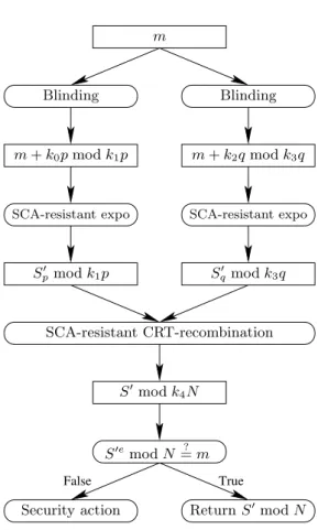
L’impact d’un tel résultat en cryptanalyse est immédiat car il permet d’attaquer RSA lorsque l’attaquant a obtenu, par exemple, des informations partielles sur la clé privée à l’aide d’une analyse par canaux auxiliaires. L’idée de base de Coppersmith pour résoudre ce problème peut s’exprimer de la manière suivante : comme il est difficile de trouver la solution x d’une équation
8 CHAPITRE1. Introduction et Synthèse
Algorithme 1: Algorithme de Coppersmith
entrée: Un problème Dioph(1, d, N) modélisé par f
sortie : Une petite racine entière x à ce problème, si elle existe
À partir de f on engendre un certain nombre de polynômes gis’annulant en x modulo Nh;
Des coefficients des gion déduit la base B d’un réseau euclidien L;
(*) On extrait un vecteur suffisamment court v du réseau L; On construit un polynôme F dont les coefficients sont déduits de v;
La solution x doit être une racine de F vu comme un polynôme à coefficients entiers; retourne x si elle a été trouvée à la dernière étape
FIGURE1.1 – Résolution du problème 3
modulaire, essayons de trouver un polynôme en une variable qui s’annule en x sur les entiers. L’outil algorithmique permettant ce calcul est la réduction d’un réseau euclidien construit à partir de l’équation de départ. L’algorithme peut se résumer comme suit.
L’étape marquée d’un astérisque est a priori de complexité exponentielle. En effet, trouver trouver un vecteur court dans un réseau est connu pour être NP-difficile depuis les travaux de Ajtai. Toute la subtilité se trouve dans le suffisamment court. Coppersmith utilise l’algorithme LLL [104] pour réduire la base B et prend pour v le vecteur le plus court issu de cette réduction. Ce calcul se faisant en temps polynomial et il montre que si l’ensemble des gi est bien choisi, même si v est une approximation exponentiellement mauvaise d’un vrai vecteur court de L, elle suffit à résoudre le problème 3. Plus généralement cette approche peut être adaptée pour trouver des petites racines à des problèmes Dioph(n, d, N). En particulier Coppersmith donne un algorithme dans [34] pour résoudre en temps polynomial le cas Dioph(2, d, 1). Dans les autres cas, les approches sont à ce jour toujours heuristiques.
Le résultat majeur que nous avons obtenu dans ce contexte est l’amélioration de l’algo-rithme 1 de Coppersmith. Nous montrons dans [15] comment la structure de la base B du réseau euclidien utilisé dans cet algorithme permet d’en améliorer son efficacité. Plus exactement, nous utilisons un calcul approché par troncature (on ne garde que les parties hautes des coordonnées des éléments de B) pour effectuer la réduction de réseau. Ce calcul permettant d’obtenir le résul-tat escompté puisque nous montrons que B est triangulaire à diagonale équilibrée. Aussi, nous mettons en évidence une structure cachée reliant différentes versions de la base B pour accélérer la phase énumérative de l’algorithme. Cette phase est nécessaire si l’on souhaite obtenir des so-lutions atteignant la borne théorique. Le gain en complexité est de l’ordre de log2(N )/d2 et les gains pratiques sont de l’ordre de plusieurs centaines pour des modules N de tailles 1024 bits.
Dans l’article [6] nous montrons comment terminer une attaque combinée sur une implan-tation de RSA-CRT. Plus exactement, nous montrons comment récupérer la clé privée malgré l’application de contremesures contre les attaques par observation (de la consommation de cou-rant par exemple) et celles par injection de fautes. Notre résultat repose sur l’hypothèse que l’at-taquant est capable d’effectuer deux telles attaques au cours de la même exécution. Hypothèse réalisable en pratique aujourd’hui. L’algorithme 1 de Coppersmith est utilisé ici pour accélérer les calculs (seulement la moitié du secret doit être retrouvée grâce aux canaux auxiliaires) et ainsi
1.4. Problèmes PoSSo 9 diviser par deux le temps total de l’attaque (on passe de deux heures à une heure).
Dans [38] nous attaquons le problème de la factorisation d’entier de la forme prqs avec p et q premiers et r et s suffisamment grand. Cet article résout un problème laissé ouvert dans [23] et répond à la question de savoir si de tels modules pouvaient être utilisés dans des versions plus efficaces de RSA. Nous montrons qu’une telle factorisation est possible en temps polynomial dès que r log3(p). Ce résultat de complexité est essentiellement asymptotique, des exposants aussi grands ne peuvent être utilisés en pratique. Il a tout de même le mérite de montrer une potentielle faiblesse de RSA pour de tels modules. Un des ingrédients permettant d’arriver à nos fins est l’algorithme de Coppersmith.
Dans l’article [66], nous nous attaquons au problème de la factorisation implicite introduit par May et Ritzenhofen dans [110]. Ce problème, dans le cas de deux modules, suppose que deux entiers RSA N1 = p1q1, N2 = p2q2 sont tels que p1 et p2partagent une partie s de bits de poids forts en commun. L’attaquant ne connaît pas la valeur exacte de s, il a juste connaissance de l’existence de cette partie commune. L’attaque peut alors se modéliser facilement sous la forme d’un problème du type Dioph(3, 3, 1) défini par le polynôme
f (x, y1, y2) = y1y2x + y1N2 y2N1
dont les solutions sont ( ˜p1 p˜2, q1, q2) où ˜pi = pi s. Ainsi dès que la partie partagée s est suffisamment grande et les qi suffisamment petits, cette solution devient une petite solution du problème et une stratégie à la Coppersmith peut être appliquée. C’est cette méthode heuristique que proposent Sarkar et Maitra dans [134]. Dans [66] nous exhibons un réseau euclidien dont un court vecteur contient une solution au problème. Ainsi nous obtenons un algorithme plus efficace pour résoudre le problème en général et qui devient déterministe dans le cas de deux modules. Par rapport à May et Ritzenhofen dans [110] où ils traitaient le cas du bloc partagé de poids faible, dans [66] nous montrons comment réaliser l’attaque pour des blocs situés n’importe où dans p1 et p2.
Dans l’article [64] nous considérons une hypothèse implicite au moment de la génération des aléas utilisés pour réaliser des signatures avec (EC)DSA (égalité entre certains bits de plusieurs aléas sans connaître leur valeur exacte). Nous montrons que cette hypothèse suffit à obtenir des résultats équivalents à ceux obtenus par Nguyen et Shparlinski dans [117] où l’attaquant avait la connaissance de certains bits des aléas (voir aussi les résultats récents [4, 81]).
La conférence invitée [129] reprend quelques résultats présentés ici. Au chapitre 3 une partie des travaux [15, 6] sera détaillée et les articles [66, 64] sont donnés en annexe.
1.4 Problèmes PoSSo
Les travaux présentés ici ont été réalisés avec Claude Carlet, Jean-Charles Faugère, Pier-rick Gaudry, Christopher Goyet, Louise Huot, Antoine Joux, Christophe Petit, Ludovic Perret et Vanessa Vitse.
10 CHAPITRE1. Introduction et Synthèse
On s’intéresse ici à la résolution de systèmes polynomiaux ayant un nombre fini de solutions. Plus exactement, on cherche à représenter les solutions d’un tel système pour qu’elles puissent être extraites facilement. Dans le cadre applicatif qui nous intéresse ici, on spécifie le corps de base K à un corps fini. Certains résultats s’étendent au corps des rationnels par exemple. Le problème général s’énonce donc ainsi.
Problème 4. Étant donné un système de polynômes ayant un nombre fini de solutions toutes simples
S : {f1 =· · · = fs= 0}
avec f1, . . . , fs 2 K[x1, . . . , xn]. On demande de trouver n polynômes en une variable hi 2 K[xi] tels que les solutions de S soient en bijection avec celles de
{x1 h1(xn) = · · · = xn 1 hn 1(xn) = hn(xn) = 0} .
Clairement, lorsque l’on obtient une représentation des racines de S comme spécifiées dans le problème précédent, les solutions peuvent être listées facilement après la factorisation du po-lynômes hn. La complexité de cette énumération est polynomiale en le degré D de hn(à noter que les polynômes hi (i < n) ont un degré borné par D puisqu’ils peuvent être réduits modulo hn). De plus, si l’on cherche les racines dans K (qui est un corps fini), cette complexité (voir [76]) est de l’ordre de eO(D)opérations arithmétiques (où la notation eOsignifie que les facteurs logarithmiques en D et polynomiaux en n sont négligés). Puisque le polynôme hnencode toutes ces solutions, il est clair que le degré D représente aussi le nombre total des solutions du système S.
Pour résoudre le problème 4, l’outil algorithmique de base est le calcul de bases de Gröbner. D’après les travaux de Lakshman et Lazard [96], la complexité de ce calcul est polynomiale en D. Plus exactement, l’algorithme [63] utilisé classiquement aujourd’hui pour résoudre ce problème peut être décrit comme suit :
Algorithme 2: Résolution PoSSo
entrée: Un système S ⇢ K[x1, . . . , xn].
sortie : Une base de Gröbner pour LEX de S donnant la représentation souhaitée des solutions de S. Calcul d’une base de Gröbner pour l’ordre DRL de hSi;
À partir de la base de Gröbner DRL, calculer une base de Gröbner LEX de hSi; retourne la base de Gröbner LEX pour S
FIGURE1.2 – Résolution du problème 4
La première étape est un calcul de base de Gröbner, la seconde un calcul de changement d’ordre. On procède ainsi pour maîtriser au mieux les degrés des polynômes apparaissant au cours de la première étape et ainsi obtenir une meilleure complexité. Les meilleurs algorithmes pour résoudre cette étape sont dûs à Faugère [56, 57] et ont une complexité, sous une hypothèse de régularité du système donné en entrée, de l’ordre de O(D!). (Ici pour simplifier les études
1.4. Problèmes PoSSo 11 de complexité, on suppose que le nombre de solutions D est maximal, i.e. il atteint la borne de Bézout, ce qui est une situation générique.)
La seconde étape repose essentiellement sur des calculs d’algèbre linéaire dans le quotient K[x1, . . . , xn]/hSi ; calculs rendus possibles grâce à la base de Gröbner DRL calculée à l’étape précédente. L’algorithme FGLM introduit dans [63] permettant un tel changement d’ordre a une complexité de O(nD3).
Le fait que la base de Gröbner LEX fournisse la sortie attendue au problème 4 est soumis à une hypothèse particulière. Cette forme attendue est appelée Shape Position et on peut montrer qu’après un changement de coordonnées générique, on peut toujours se ramener à cette situation [95, 80, 11]. On peut donc supposer que la base de Gröbner LEX ainsi calculée est bien en Shape Position.
Ainsi, nous déduisons, sous des hypothèses de régularité pour le système donné en entrée et de Shape Position pour la sortie, que le problème 4 peut être résolu en temps O(nD3). En effet, c’est la seconde étape qui domine le calcul.
Dans certains contextes, il est possible d’obtenir une meilleure complexité. Par exemple, pour la recherche de racines réelles d’un système de polynômes, il est possible de les calculer en O(12nD2)lorsqu’elles sont en nombre logarithmique en D [112]. Ou encore, lorsque la structure multiplicative du quotient est connue, alors il est possible (voir [26]) de résoudre le problème 4 en O⇣n2nD52⌘. Dans [55] Faugère et Mou proposent un algorithme essentiellement quadratique en D pour le changement d’ordre mais repose sur l’exploitation de la structure potentiellement creuse des matrices apparaissant en cours de calcul. Mais en toute généralité, avant le résultat [61] la meilleure complexité connue était essentiellement cubique en D.
En effet, dans [61] (voir aussi la version étendue [60]) nous proposons un nouvel algorithme de changement d’ordre permettant de résoudre efficacement la seconde étape de l’algorithme 2. Cet algorithme fournit le premier résultat de complexité sous cubique depuis l’introduction de l’algorithme FGLM [63] et ainsi ramène la résolution du problème 4 à une complexité de eO(D!) au total. L’ingrédient clé qui nous a permis de passer d’une complexité cubique à D!est l’adap-tation de [55] en utilisant un résultat de Keller-Gehrig [92] pour le calcul rapide de produits de matrices par des vecteurs. L’utilisation d’une structure particulière des bases DRL est aussi essentielle à notre algorithme puisqu’elle permet de se passer d’une bonne part des calculs nor-malement nécessaires dans [63].
Les autres résultats de cette section se focalisent sur la première étape de l’algorithme 2. L’ar-ticle [62] peut être vu comme un des plus marquants. Il décrit une étude complète sur l’utilisation des structures liées à des actions de groupes sur les générateurs d’un idéal. Le problème sous-jacent à cette étude est issu d’un problème intervenant dans le calcul d’indice pour la résolution du problème du logarithme discret (DLP) sur les courbes elliptiques. Les meilleurs algorithmes connus pour résoudre ce problème sont de complexité exponentielle. Nous montrons comment les points de 2-torsion permettent de gagner un facteur exponentiel par rapport aux travaux de Gaudry et Diem [78, 48, 47].
L’étude précédente est réalisée pour des corps finis de grande caractéristique, dans [65] nous étendons ces résultats au cas de la caractéristique 2. Un autre résultat important de cet article
12 CHAPITRE1. Introduction et Synthèse
est le record de calcul réalisé lors de ce travail. En effet, dans ce contexte, la modélisation du problème DLP passe par le calcul d’un polynôme de sommation en n+1 variables pour résoudre le problème de décomposition en n points. Aucun polynôme de sommation pour n > 6 n’avait jamais été calculé, ici nous montrons comment l’utilisation des symétries permet de calculer celui pour n = 8 en une quarantaine d’heures de calcul. Sachant que le précédent est calculable en 380 secondes, on se rend bien compte du caractère exponentiel de ce calcul. Les techniques utilisées pour arriver au bout de ce calcul sont issus du calcul formel et plus particulièrement de résultats de l’interpolation rapide de polynômes.
L’article [68] présente une étude préliminaire sur la résolution du DLP sur les courbes el-liptiques en caractéristique 2 basée sur une version de du calcul d’indice dû à Diem [48, 47]. L’utilisation de la résolution des systèmes polynomiaux est central. Ici aucune hypothèse n’est faite sur la nature du corps de base (en particulier l’extension peut être de degré premier). Nous montrons que les systèmes polynomiaux intervenant dans cette étude possèdent une structure multi-homogène et obtenons ainsi une amélioration en complexité par rapport aux résultats de Diem. Cependant, ceci ne nous permet pas de montrer que cette approche est meilleure que les résolutions génériques du DLP. En effet, nous mettons aussi en évidence la présence de chutes de degrés lors de la résolution de ces systèmes. Ceci montre en particulier qu’il est difficile d’en-visager un gain conséquent en efficacité sans utiliser plus de structures spécifiques au problème (comme nous l’avons fait dans [65]).
Dans [30] nous étudions la résolution des systèmes issus de l’analyse de sécurité de chiffre-ment par blocs. Nous étudions en particulier les structures des systèmes obtenus à l’aide d’at-taques par canaux auxiliaires ; les observations physiques permettant de récupérer les poids de Hamming de secrets tout au long du calcul. Nous déduisons de cette étude un critère permettant d’évaluer la sécurité des boite-S (briques de base des chiffrements par bloc) face à des attaques combinant l’approche algébrique et des informations issues d’attaques par canaux auxiliaires.
Ces travaux furent présentés lors de conférences invitées [128, 127]. Au chapitre 4 une partie des travaux [62, 65] sera détaillée. Les articles [30] et [61] sont donnés en annexe.
1.5. Liste des publications depuis 2006 13
1.5 Liste des publications depuis 2006
Pour faciliter l’identification des articles publiés après ma thèse (2006), ils sont listés ci-après. Ils sont aussi rappelés, avec la même numérotation, dans la bibliographie à la fin de ce document. Dans la version numérique de ce document, des liens hypertexte dans chacune de ces références permettent d’obtenir les publications correspondantes (et les slides pour certains cours ou conférences invitées).
Revues internationales avec comité de lecture
[30] Claude CARLET, Jean-Charles FAUGÈRE, Christopher GOYET et Guénaël RENAULT.
“Analysis of the algebraic side channel attack”. In : J. Cryptographic Engineering 2.1 (2012).PDF, p. 45–62.
[62] Jean-Charles FAUGÈRE, Pierrick GAUDRY, Louise HUOTet Guénaël RENAULT. “Using
Symmetries in the Index Calculus for Elliptic Curves Discrete Logarithm”. In : J. Cryp-tology 27.4 (2014).PDF, p. 595–635.
[93] Masanari KIDA, Guénaël RENAULT et Kazuhiro YOKOYAMA. “Quintic polynomials of
Hashimoto-Tsunogai, Brumer and Kummer”. In : Int. J. Number Theory 5.4 (2009).PDF, p. 555–571. ISSN: 1793-0421.
[121] Sébastien ORANGE, Guénaël RENAULTet Kazuhiro YOKOYAMA. “Efficient arithmetic
in successive algebraic extension fields using symmetries”. In : Math. Comput. Sci. 6.3 (2012).PDF, p. 217–233.ISSN: 1661-8270.
Actes de conférences internationales avec comité de programme
[6] Guillaume BARBU, Alberto BATTISTELLO, Guillaume DABOSVILLE, Christophe GI -RAUD, Guénaël RENAULT, Soline RENNER et Rina ZEITOUN. “Combined Attack onCRT-RSA - Why Public Verification Must Not Be Public?” In : Public-Key Cryptogra-phy - PKC 2013 - 16th International Conference on Practice and Theory in Public-Key Cryptography, Nara, Japan, February 26 - March 1, 2013. Proceedings. PDF. 2013, p. 198–215.
[15] Jingguo BI, Jean-Sébastien CORON, Jean-Charles FAUGÈRE, Phong Q. NGUYEN,
Gué-naël RENAULT et Rina ZEITOUN. “Rounding and Chaining LLL: Finding Faster Small
Roots of Univariate Polynomial Congruences”. In : Public-Key Cryptography - PKC 2014 - 17th International Conference on Practice and Theory in Public-Key Cryptogra-phy, Buenos Aires, Argentina, March 26-28, 2014. Proceedings.PDF. 2014, p. 185–202.
14 Actes de conférences internationales avec comité de programme [38] Jean-Sébastien CORON, Jean-Charles FAUGÈRE, Guénaël RENAULT et Rina ZEITOUN.
“Factoring N = prqsfor Large r and s”. In : Topics in Cryptology - CT-RSA 2016 - The Cryptographers’ Track at the RSA Conference 2016, San Francisco, CA, USA, February 29 - March 4, 2016, Proceedings.PDF. 2016, p. 448–464.
[61] Jean-Charles FAUGÈRE, Pierrick GAUDRY, Louise HUOT et Guénaël RENAULT.
“Sub-cubic change of ordering for Gröbner basis: a probabilistic approach”. In : International Symposium on Symbolic and Algebraic Computation, ISSAC ’14, Kobe, Japan, July 23-25, 2014.PDF. 2014, p. 170–177.
[64] Jean-Charles FAUGÈRE, Christopher GOYETet Guénaël RENAULT. “Attacking (EC)DSA
Given Only an Implicit Hint”. In : Selected Areas in Cryptography, 19th International Conference, SAC 2012, Windsor, ON, Canada, August 15-16, 2012, Revised Selected Pa-pers.PDF. 2012, p. 252–274.
[65] Jean-Charles FAUGÈRE, Louise HUOT, Antoine JOUX, Guénaël RENAULT et Vanessa
VITSE. “Symmetrized Summation Polynomials: Using Small Order Torsion Points to
Speed Up Elliptic Curve Index Calculus”. In : Advances in Cryptology - EUROCRYPT 2014 - 33rd Annual International Conference on the Theory and Applications of Crypto-graphic Techniques, Copenhagen, Denmark, May 11-15, 2014. Proceedings.PDF. 2014, p. 40–57.
[66] Jean-Charles FAUGÈRE, Raphaël MARINIER et Guénaël RENAULT. “Implicit Factoring
with Shared Most Significant and Middle Bits”. In : Public Key Cryptography - PKC 2010, 13th International Conference on Practice and Theory in Public Key Cryptogra-phy, Paris, France, May 26-28, 2010. Proceedings.PDF. 2010, p. 70–87.
[68] Jean-Charles FAUGÈRE, Ludovic PERRET, Christophe PETITet Guénaël RENAULT.
“Im-proving the Complexity of Index Calculus Algorithms in Elliptic Curves over Binary Fields”. In : Advances in Cryptology - EUROCRYPT 2012 - 31st Annual International Conference on the Theory and Applications of Cryptographic Techniques, Cambridge, UK, April 15-19, 2012. Proceedings.PDF. 2012, p. 27–44.
[90] Jean-Gabriel KAMMERER, Reynald LERCIER et Guénaël RENAULT. “Encoding points
on hyperelliptic curves over finite fields in deterministic polynomial time”. In : Pairing-based cryptography—Pairing 2010. T. 6487. Lecture Notes in Comput. Sci.PDF. Sprin-ger, Berlin, 2010, p. 278–297.
[120] Sébastien ORANGE, Guénaël RENAULTet Kazuhiro YOKOYAMA. “Computation schemes
for splitting fields of polynomials”. In : ISSAC 2009—Proceedings of the 2009 Internatio-nal Symposium on Symbolic and Algebraic Computation.PDF. ACM, New York, 2009, p. 279–286.
[132] Guénaël RENAULT et Kazuhiro YOKOYAMA. “Multi-modular algorithm for computing
the splitting field of a polynomial”. In : ISSAC 2008. PDF. ACM, New York, 2008, p. 247–254.
Travaux récents, cours et conférences invités, posters 15
Travaux récents, cours et conférences invités, posters
[9] Lucas BARTHÉLÉMY, Ninon EYROLLES, Guénaël RENAULT et Raphaël ROBLIN.
“Bi-nary Permutation Polynomial Inversion and Application to Obfuscation Techniques”. In : To appear in 2nd ACM International Workshop on Software Protection, SPRO 2016, Vienna, Austria, October 28, 2016.PDF. 2016, p. 1–9.
[60] Jean-Charles FAUGÈRE, Pierrick GAUDRY, Louise HUOT et Guénaël RENAULT.
Poly-nomial Systems Solving by Fast Linear Algebra.PDF. 2013.
[130] Guénaël RENAULTet Tristan VACCON. “On the p-adic stability of the FGLM algorithm”.
In : CoRR abs/1602.00848 (2016).PDF.
[125] Guénaël RENAULT. “Introduction à la Théorie de Galois Effective”. In : JNCF’08:
Jour-nées Nationales du Calcul Formel (online). PDF, Slides. Marseille, France, oct. 2008, p. 141–197.
[126] Guénaël RENAULT. Introduction à l’Algorithmique Galoisienne. Invited talk at
Mathe-matik Park (Institut Henri Poincaré),Slides. 2011.
[127] Guénaël RENAULT. On polynomial systems with structures related to the ECDLP. Invited
talk during the Conference Effective Moduli Spaces and Applications to Cryptography (Rennes, France). 2014.
[128] Guénaël RENAULT. On Using Torsion Points in the Elliptic Curve Index Calculus. Invited
talk during the 18th Workshop On Elliptic Curve Cryptography (ECC 2014), Slides. 2014.
[129] Guénaël RENAULT. The Heuristic Coppersmith Technique from a Computer Algebra
Point of View. Invited talk during the SIAM Conference on Applied Algebraic Geometry (Fort Collins, Colorado, USA),Slides. 2013.
[59] Jean-Charles FAUGÈRE, Pierrick GAUDRY, Louise HUOTet Guénaël RENAULT. “Fast
change of ordering with exponent !”. In : (Poster abstract) ACM Commun. Comput. Algebra 46 (sept. 2012).PDF, p. 92–93.
C
HAPTER
2
Contribution to Effective Galois Theory
In this chapter, some results on the computation of the roots of a univariate polynomial are presented. They are all related to Problem 1 introduced in Chapter 1. Our papers corresponding to the subject of this chapter are [121, 90, 120, 93, 132, 125]. In the sequel, we detail the results of [120, 90].
2.1 Introduction
In Section 2.2 we consider the problem of computing efficiently the splitting field of a uni-variate polynomial f 2 K[x]. A well known bootstrapping algorithm for this task consists of factoring f over K1 =K[t]/f(t), adjoining a root of f to K, computing a primitive element for this field over K, and repeating this procedure until f splits completely. This simple algorithm has a running time which is polynomial in the size of f (the L2-norm of its coefficients) and the size of its Galois group. In general, this is the best we can do for this computation (see [97, 98]). In the articles [132, 131, 124], we presented some techniques, obtained from the action of the Galois group, which help such a computation and we also use them when this representation is computed by interpolation. In this chapter, we give a general presentation of these techniques and we present a complexity result (see Theorem 2.10) stating that their computation do not impact the global cost of the computation. In practice, the use of these techniques provides a speed-up of a factor up to several hundreds. These results are part of the article [93].
Another way of representing roots of a univariate polynomial is, when it is possible, by radi-cals. In Section 2.3, we present some applications in cryptography of such a representation. The main result of this part (coming from [90]) is Theorem 2.13 stating that a family of polynomials with solvable Galois group can be used to define an encoding on an hyperelliptic curve. These encodings are deterministic and thus avoid possible leaks of secret during the computation. Such a property is of great importance in the context of embedded cryptography where an attacker can “listen” the chip during the encryption/decryption phase.
18 CHAPTER2. Contribution to Effective Galois Theory
2.2 Splitting field computation
The computation of the splitting field of a polynomial f plays an important role in Galois theory and more generally in algorithmic number theory. It is the smallest field where all the roots of f lie. Providing a suitable representation of this field allows symbolic computations with all the roots of the polynomial and thus provides a solution to the problem 1.
Such a representation comes from computer algebra and more precisely from Gröbner basis theory. Let f be a univariate irreducible and separable polynomial of degree n with coefficients in a field K and ↵1, . . . , ↵n its roots. A natural representation of the splitting field of f is the quotient algebra
K(↵1, . . . , ↵n)' K[x1, . . . , xn]/M
where M is the kernel of the surjective morphism from K[x1, . . . , xn]to K(↵1, . . . , ↵n) which maps xi to ↵i. The ideal M, called a splitting ideal of f, is zero-dimensional and maximal. Knowing a Gröbner basis of M allows computations in this quotient algebra by means of linear algebra operations (e.g. [42, 12]) and then symbolic operations with the roots of f.
In [132] we propose an algorithm for computing the splitting field of a monic irreducible polynomial f with coefficients in K = Q (more generally, these methods can be applied in any global field). This algorithm takes as input the polynomial f and, as a first preparatory step, computes the action of its Galois group over p-adic approximations of its roots. The other steps are based on the relationship between the representation of the splitting field by a Gröbner basis and the action of the corresponding Galois group on this basis. The core of this new approach, called computation scheme (see section 2.2.1), uses the internal symmetries of the problem in order to speed up the Gröbner basis computation. This scheme is computed from the knowledge of a permutation representation of the Galois group G of f and provides a shape of the Gröbner basis of the splitting ideal of f. From this shape, the algorithm effectively computes the basis by interpolating its coefficients (see also [111, 144, 123, 103] and more generally [44] for interpolation strategies). Our general method can be depicted as the following drawing.
Computation of the set T
[ R., Yokoyama ANTS’06][ R., Yokoyama ISSAC’08]:
Interpolation
with a
careful treatment
on reducing computational difficulty
(introduction of the
computation schemes
).
Input Computation Scheme Computation Output
f
Galois Group ComputationG
f· (↵
1, . . . , ↵
n)
mod p
8 < : g1(x1) g2(x1, x2) .. . gn(x1, . . . , xn) The triangular setC
8 < : g1= x81+ . . . g2= x62+ . . . g3= x43+ . . . g4= x24+ . . . g5= x15+ . . . g6= x16+ . . . g7= x17+ . . . g8= x18+ . . .T
From the Galois group
P
c
ix
k11· · · x
knnForm of g
i=
Interpolation + Hensel Liftg
iThe total efficiency of the computation relies on the computation
scheme !
7/23
The efficiency of this algorithm heavily depends on this computation scheme which depends itself on the choice of the representative of the conjugacy class of G in Sn. When we choose the best representative of a given permutation group, the gain in efficiency may be very large.
2.2. Splitting field computation 19 Actually, this can be measured as a function of the number of coefficients we need to compute by interpolation. Without using the computation scheme, this number is bounded by |nG| the size of the group times its degree. Using the computation scheme, this number can be reduced to a function c(G) depending on G, for example we have the following comparison table.
Group 7T6 8T48 9T25 9T29 9T32 10T36 10T39 nG 7⇥ 2520 8 ⇥ 1344 9 ⇥ 324 9⇥ 648 9⇥ 1512 10 ⇥ 1920 10 ⇥ 3840 c(G) 2520 336 27 18 + 648 2⇥ 1512 10 + 960 10 As one can see, depending on the group G, this gain of efficiency may be huge. The problem is that the quantity c(G) does not depends on G only but on its representative. Thus, finding this representative may have a combinatorial cost. In [131, 132] we overcome this problem by tabulating these best representatives. From an algorithmic point of view, tabulating is not really satisfying, thus we propose in [120] a method which efficiently identifies such representatives. We present this method in the sequel.
2.2.1 Computation schemes
For the natural group action of Snon Q[x1, . . . , xn]which permutes the xi’s by acting on the indices, the stabilizer of M is the permutation representation of the Galois group which will be denoted by G:
G ={ 2 Sn| 8g 2 M, .g 2 M}.
Proposition 2.1. Let be a permutation of Sn and let G = G 1. The ideal .M = { .f | f 2 M} is the splitting ideal corresponding to the roots .↵ = (↵ .1, . . . , ↵ .n) and the corresponding representation of the Galois group is G (a conjugate of G).
A first result coming from classical Galois theory (see for example [144]) shows that the basis G of M is triangular for the lexicographical order induced by x1 <· · · < xn(see [100]). That is, G is given as a set of n polynomials {f1, . . . , fn} such that fi has a power of xi as leading term and is separable as a polynomial in xi. Moreover, we can deduce from G the degree di of the leading term of each fi. Let E be a subset of {1, . . . , n}, we denote by StabG(E)the pointwise stabilizer in G of E (that is the subgroup of G given by { 2 G | (e) = e 8e 2 E}). We have the following classical result:
di =| StabG({1, 2, . . . , i 1}|/| StabG({1, 2, . . . , i})|. (2.2.1) Thus, the degrees di of elements in a Gröbner basis (not necessarily reduced but minimal) G of M can be deduced only from the stabilizer G of this ideal. This result gives a very general shape for G. In the sequel we show how to improve this shape by inspecting the property of G.
Let i be an integer in [[1, n]]. A sequence r of couples [(i1, k1), (i2, k2), . . . , (is, ks)] with {i1 < i2 < . . . < is = i} a part of {1, . . . , i} and kj 6 dij is said to be an i-relation if there
exists a polynomial gi 2 K[xi1, . . . , xis]such that ↵
ki+1
i + gi(↵1, . . . ↵i) = 0with degxij(gi)6 kj (note that we must have ki = kis = di 1and kj < dij for j < s). The polynomial gi is called
the the tail polynomial of this i-relation. Since the i-relation depends on the roots ↵1, . . . , ↵n, the existence of a given i-relation depends only of the Galois group G, more exactly we have:
20 CHAPTER2. Contribution to Effective Galois Theory
Proposition 2.2. There exists an i-relation [(i1, k1), . . . , (is, ks)]as soon as 8j 2 [[1, s]], kj = | Stab| StabGG({i({i1,...,i1,...,ijj)1}|})| and | Stab| StabGG({i({i1,...,i1,...,is 1s)}|})| = di.
An important quantity attached to an i-relation is its size which corresponds to the product ki1⇥ · · · ⇥ kis and represents the maximal number of monomials of the corresponding
polynomi-als fi. Thus, in order to minimize the cost for computing the triangular basis G by indeterminate coefficients strategy, we need to know the best i-relation possible, that is the one with mini-mal size. Such an i-relation is said to be minimal. We now see how to avoid some of these computations by using two techniques.
The computation scheme can be seen as a set of techniques which help to compute G from G. The first technique, calledCauchy technique, is based on the so called generalized Cauchy modules (see [123]):
Definition 2.3. Let G = {f1, . . . fn} be a triangular basis of M and {i = i1 < · · · < ir} the orbit of i under the action of StabG({1, . . . , i 1}). The di generalized Cauchy modules of fi are inductively defined by Ci1(fi) = fi(xi1)and for k > 2 the polynomial Ci1, . . . ,ik(fi)is given
by the divided difference
Ci1, . . . ,ik 1(fi)(xik) Ci1,...,ik 1(fi)(xik 1)
xik xik 1
.
From these constructions, we can deduce polynomials of G from other ones. The following result explains this relation.
Proposition 2.4. The Cauchy module Ci1,...,ik(fi)is a polynomial of K[x1, . . . , xik]and its
lead-ing term is xdi k+1
ij . Moreover, Ci1, . . . ,ik(fi)belongs to M. In particular, if di k + 1 = dik
then
{f1, . . . , fik 1, Ci1,...,ik(fi), fik+1, . . . , fn}
is a triangular basis of M.
Cauchy, in [31, Extrait 108], already proved similar results (without the knowledge of Gröb-ner basis theory) when he studied the application of Ampère’s ¨fonctions interpolaires¨ (what we call now Cauchy modules) for eliminating variables in symmetric funtions.
The second technique considers the natural action of G over the polynomials of G (permuta-tions of the indexes of the variables) to find rela(permuta-tions between these polynomials. These special permutations are namedtransporters.
Definition 2.5. Let [(i1, k1), . . . , (is, ks)] be an i-relation and j 2 [[i + 1, n]]. A permutation 2 G is called an (i, j)-transporter if (i) = j and j = max( (k) | k 2 {i1, . . . , is}).
As for Cauchy technique, transporters can be used to produce, without any cost, polynomials of G from others taken in G:
2.2. Splitting field computation 21 Proposition 2.6. Let be an (i, j)-transporter and gi 2 K[xi1, . . . , xis] the tail polynomial
corresponding to fi. If di = dj then {f1, . . . , fj 1, xdjj+ .gi, fj+1, . . . , fn} is a triangular basis of M.
All these techniques and the i-relations can be deduced only by inspecting the corresponding permutation group G. Thus, we can now define its corresponding computation scheme.
Definition 2.7. The computation scheme of the permutation group G is defined by the following data:
1. the degree di of the greatest variable in each polynomial in G;
2. mathematical objects (shape) computed by Cauchy techniques and transportation ;
3. the minimal i-relation of each polynomial in G that can not be obtained by the preceding techniques.
The c-size of this computation scheme, denoted by c(G), is defined by the number of monomials over all the i-monomials in 3.
⌅
⌅
⌅
⌅
⌅
⌅
⌅
⌅
⌅
⌅
⌅
⌅
⇤
⌅
⌅
⌅
⌅
⌅
⌅
⌅
⌅
⌅
⌅
⌅
⌅
⇥
f
1= x
81+ ...
f
2= x
12+ ...
f
3= x
63+ ...
f
4= x
14+ ...
f
5= x
45+ ...
f
6= x
16+ ...
f
7= x
27+ ...
f
8= x
18+ ...
⌅
⌅
⌅
⌅
⌅
⌅
⌅
⌅
⌅
⌅
⌅
⌅
⇤
⌅
⌅
⌅
⌅
⌅
⌅
⌅
⌅
⌅
⌅
⌅
⌅
⇥
f
1= x
81+ ...
f
2= x
62+ ...
f
3= x
43+ ...
f
4= x
24+ ...
f
5= x
15+ ...
f
6= x
16+ ...
f
7= x
17+ ...
f
8= x
18+ ...
Cauchy 48 192 284 8 Transporters Cauchy Transporters 8The c-size c(G) represents the total num-ber of coefficients to compute in order to retrieve the triangular basis G by interpola-tion. The main drawback of the computation scheme is that it is dependent of the choice of the representative for the group G.
For example, let
G1 =h(8, 7, 6, 1)(5, 4, 3, 2), (8, 1)(4, 5), (5, 1)i and
G2 =h(2, 1), (8, 6, 4, 1)(7, 5, 3, 2), (8, 1)(7, 2)i be two conjugates in S8 of the transitive per-mutation group [24]S
4.
The two corresponding computation schemes can be represented by the following drawings
(G1 on the left and G2 on the right). On these drawings, the techniques are showed on the left side of the triangular bases and the integers, on right side, represents the sizes of the minimal i-relations. Thus, for G1we have c(G1) = 532and for G2we obtain only c(G2) = 8.
Thus, in order to obtain the best efficiency by using computations schemes, we need a method which identifies the representative of a given group which provides a scheme with minimal c-size.
Computation of Computation Schemes
A brute force method is proposed in [123] for computing a conjugate of a permutation group with minimal computation scheme in the sense of the c-size. In this method, the number of candidates considered is equal to the index |Sn : NSn(G)| which can be closed to (n 1)! when G
is moderate (in particular for the cyclic group of degree n, this index is equal to (n 1)!
(n) ). Thus the brute force method is completely useless in this case. In [120], we show how to easily construct a
22 CHAPTER2. Contribution to Effective Galois Theory
computation scheme for particular types of permutation group. Also, we provide a data-structure which can be constructed for any type of permutation group and helps in finding such a minimal computation scheme. The concept of this data-structure is based on the correspondence between the sequence of pointwise stabilizer subgroups orbits of G and the sequence of factors of a polynomial f with Galois group G in the tower of subfields arising during the computation of its splitting field.
In fact, the two computations schemes techniques and minimal i-relations depend only on the structure of the different orbits of the pointwise stabilizers of G which correspond to the different factors arising during the computation of the splitting field by successive factorization.
Thus we do not need to inspect all the conjugates of a group but all the different possible sequences of orbits appearing during the process of stabilization of the group G. Then, from all these possibilities we well order the choice of the orbits to obtain the best conjugate of G in regards of its computation scheme. All these possibilities corresponds to a set of different classes of non redundant bases of G:
Definition 2.8. Let G be a permutation group of degree n. A sequence B = (b1, . . . , bk) of different integers from {1, . . . , n} is called a regular sequence of length k. A regular sequence B is said to benon redundant with respect to G if
G = G[1]B > G[2]B >· · · > G[k+1]B , where, we denote by G[i]
B (i> 2) the pointwise stabilizer StabG({b1, . . . , bi 1}) in G. Moreover, for a non redundant regular sequence B, if G[k+1]
B = 1, B is said to be anon redundant base of G. The largest k such that there is a non redundant base of length k is called thedepth of G.
Let B1 = (a1, a2, . . . , al)and B2 be two non redundant bases of G of the same length. We say that B1 is G-equivalent to B2if there exists g 2 G such that B2 = (g(a1), g(a2), . . . , g(al)) The G-equivalence property is an equivalent relation over the set of non redundant bases. In a field theory point of view, two non redundant bases are G-equivalent iff the towers of fields defined by these bases are isomomorphic level by level from the ground field Q to the splitting field. From now on, when we will speak about classes of non redundant bases they will be always classes of G-equivalence.
A data structure attached to the permutation group G is introduced. It lets us store all the non redundant bases of G and the corresponding orbits of the natural action of its stabilizer along these different bases. From now on we say that an orbit is non trivial when it is not reduced to one element. It is important to recall that G is transitive since the polynomial is supposed to be irreducible.
Definition 2.9. The orbit tree T of G is the recursive structure defined by 1. The root T (0) of T is the orbit of G: {1, . . . , n};
2. any other node T (i1 = 1, i2, . . . , is) is the set of orbits of StabG({0, i1, . . . , is}) where is is the minimal element of a non trivial orbit in the node T (i1 = 1, i2, . . . , is 1);
3. the construction is stopped as soon as the node contains only trivial orbits.
Let T (i1, . . . , is) be a node in T . The degree of this node is the integer defined by the index |G : StabG({0, i1, . . . , is})|.
2.2. Splitting field computation 23 (1)(2,5,3)(4,6,7) (1,2,3,4,5,6,7) (1)(2)(3)(4)(5)(6)(7) (1)(2)(3)(4)(5)(6)(7) T (0) T (0, 1) T (0, 1, 2) T (0, 1, 4)
For example, if G be a copy in S7 of the tran-sitive group F21(7) generated by {(1, 2, 3, 4, 5, 6, 7), (1, 2, 4)(3, 6, 5)}. The drawing on the right corresponds to its orbits tree.
From the orbits tree of a given group G, we propose an algorithm in order to find the computation scheme with smallest c-size. It proceeds in the following way: For each branch in the orbit tree.
1. Maximize the use of Cauchy technique by pro-moting linear relations first.
2. Apply Transporter technique on the remaining polynomials
3. Compute minimal i-relations for each remaining polynomials
At the end of the process the minimal computation scheme is then deduced. By using this algo-rithm we obtain the following result.
Theorem 2.10. For a given transitive permutation group G of degree n. If |G| < 2n then the computation scheme corresponding to G with minimal c-size can be computed with an algorithm of polynomial complexity in |G|.
At least this computation does affect the total cost of the procedure for the splitting field computation. But this complexity does not well reflect the impact of this strategy in practice. The cost of finding the best computation scheme is negligible in comparison with the other steps of the splitting field computation. For almost all the groups G of degree at most 15 and |G| < 10000, the timings (done with MAGMAon an 32-bit 2.5GHz Intel processor) for the computation scheme
are too small (in average < 1 second) to be really measured. Only few examples gave timings of at most 2 seconds. But, its impact on the global computation is consequent. In the following table, we show the timings (in seconds) for each step of the splitting field computation and we compare our implementation to the internal Magma function. In this table, > (resp. >>) means a timing more than 600 (resp. 2000) seconds.
Group |G| Galois Grp. Comp. Sch. Interpolation Magma
7T6 2520 0.06 0.00 52.5 > 8T32 96 0.16 0.00 0.72 33.5 8T42 288 0.1 0.00 0.18 17.9 8T47 1152 0.07 0.00 0.5 422.3 9T25 324 0.42 0.10 4.07 106.1 9T27 507 0.82 0.00 116.3 > 9T31 1296 0.32 0.10 0.5 > 9T31 1512 0.78 0.10 753.5 >>
As one can see, the part which takes most of the time is the interpolation step. Also, our approach using computation scheme is clearly better than the classical one used by Magma.
24 CHAPTER2. Contribution to Effective Galois Theory
2.3 Radical representation of roots and applications
In the preceding section we describe a general method to represent the roots of a polynomial in an effective way. In some particular cases, roots of polynomials can be represented as radicals. The problem to identify exactly which polynomials verify this property can be seen as the starting point to Galois theory. Thanks to Abel and Galois, we know today that such polynomials are the ones with a solvable Galois group. In [93] we prove isomorphism between fields defined by two different C5-generic polynomials. The core idea used in this work is the fact that the roots can be expressed as radicals, thus can be easily represented, even for a parametric polynomial. In [90] we use this fact to solve a problem related to the design of cryptographic protocols based on algebraic curves. We present a part of this work in the sequel.
Discrete Logarithm Problems based on algebraic curves on finite fields are of high interest in asymmetric cryptography. In particular they provide small size of keys needed to achieve good security. Nonetheless it is less easy to encode a message into an element of the group (in contrary to the case of DLP based on finite fields).
Let Fq be a finite field of odd characteristic p, and H/Fq : y2 = f (x)where deg f = d be an elliptic (if d = 3 or 4) or hyperelliptic (if d > 5) curve, we consider the problem of comput-ing points on H in deterministic polynomial time. In cryptographic applications, computcomput-ing a point on a (hyper)elliptic curve is a prerequisite for encoding a message into its Jacobian group. Boneh-Franklin Identity-Based Encryption scheme [24] requires for instance to associate to any user identity a point on an elliptic curve. Having such a deterministic encoding is of high impor-tance in the context of embedded implementation of cryptographic protocols. Non deterministic algorithms may leak information on secret keys.
For example, Atkin and Morain [5] remark that if x0 is any element of Fq and = f (x0), then the point ( x0, (d+1)/2)is on the curve Y2 = df (X/ )(for odd integer d). But the latter can be either isomorphic to the curve or its quadratic twist, following that is a quadratic residue or not, and we have no way to control this in deterministic time.
In 2006, Shallue and Woestjine [136] proposed the first practical deterministic algorithm to encode points into an elliptic curve, quickly generalized by Ulas [139] to the family of hyperel-liptic curves defined by y2 = xn+ ax + bor y2 = xn+ ax2+ bx. Icart [87] proposed in 2009 another deterministic encoding for elliptic curves, of complexity O(log2+o(1)q), provided that the cubic root function, inverse of x 7! x3 on F⇤
q, is a group automorphism. This encoding uses the well known radical expression of the roots of a cubic polynomial based on Cardano-Tartaglia’s formulae. It parameterizes the points (x : y : 1) on any elliptic curve E : x3 + ax + b = y2. Recall that any cubic polynomial has solvable Galois group and thus its roots can be represented as radicals and are easy parametrized as soon as the radicals are automorphisms.
In [90], we propose a general strategy based on polynomial with solvable Galois group in order to design encoding in (hyper)elliptic curves. Note that in parallel to this work and inde-pendently a different approach was proposed in [73]. Here we present only a part of [90], more exactly, we present how to design an encoding from the parametric (general) polynomial of De Moivre.
2.3. Radical representation of roots and applications 25
2.3.1 Rational and deterministic encoding from solvable polynomials
Let fa(X)be a family of parameterized polynomials (where a denotes a k-tuple (a1, a2, . . . , ak) of parameters) with solvable Galois group. We are interested in such parametric polynomials but also in the parametric radical expression of their roots a. For instance fA(X) = X2 + A in degree 2, or more interestingly fA,B(X) = X3 + A X + B in degree 3, are such polynomials with simple radical formulae for their roots. The former verifies A =
p
A and a root of the second one is given by the well-known Cardano-Tartaglia’s formulae (see [43]).
Given a parameterized family of solvable polynomials fa(X), and a genus g, we now substi-tute a rational function Fi(Y )in some variable Y for each parameter ai in a.
Let F (Y ) denote the k-tuples of rational functions (F1(Y ), F2(Y ), . . . , Fk(Y )). The equa-tion fF (Y )(X)now defines a plane algebraic curve C, with variables (X, Y ). The genus of C increases when the degrees of F (Y ) in Y increase. So if we target some fixed genus g for C, only few degrees for the numerators and denominators of F (Y ) can occur. Since we can con-sider coefficients of these rational functions as parameters b = (b1, . . . , bk0), this yields a family
of curves Cb.
Less easily, it remains then to determine among these F (Y ) the ones which yield roots F (Y ) which can be computed in deterministic time. The easiest case is probably when no square root occurs in the computation of a, since then any choice for F (Y ) will work, at the expense of some constraint on the finite field. But this is usually not the case, and we might try instead to link these square roots to some algebraic parameterization of an auxiliary algebraic curve
In some case (typically hyperelliptic curves), it is useful to derive from the equation for Cb a minimal model (typically of the form y2 = g
b(x)). In order to still have a deterministic encoding with the minimal model, we need explicit birational maps x = ⇤b(X, Y ), y = ⌦b(X, Y )too. All in all, we obtain an encoding for a minimal model gb:
— Fix some Y as a (non-rational) function of some parameter t so that all the square roots appearing in the expression of F (Y ) are well defined ;
— Compute X = F (Y );
— Compute x = ⇤b(X, Y )and y = ⌦b(X, Y ).
Once we will have found an encoding, it is important for cryptographic applications to study the cardinality of the subset of the curve that we parameterize. This ensures that we obtain convenient weak encodings for hashing into curves primitives (see [28]).
In the case of the De Moivre’s family, we are able to deduce from the encoding formulae, a polynomial relation Pb(Y, t)between any Y of a point of the image and its preimages. Then the number of possible preimages is at most the t-degree of Pb(Y, t).
We also need to know in advance which values of Fqcannot be encoded using such functions, in order to deterministically handle such cases. In the De Moivre case, this set is small.
2.3.2 De Moivre’s polynomials
This well-known family of quintic polynomials was first introduced by De Moivre in 1706 for the study of trigonometric equalities and its study from a Galoisian point of view was done by Borger in [25]. This definition can be easily generalized for any odd degree.
26 CHAPTER2. Contribution to Effective Galois Theory
Definition 2.11 (De Moivre’s polynomials). Let K be a field and d be an odd integer coprime with char K. The family of De Moivre’s polynomials pa,b(x) 2 K[x] of degree d is defined for a, b2 K by
pa,b(x) = xd+ daxd 2+ 2da2xd 4+ 3da3xd 6+· · · + 2da(d 1)/2 1x3+ da(d 1)/2x + b . Examples. De Moivre’s polynomials of degree 5 are x5+ 5ax3+ 5a2x + b. De Moivre’s poly-nomials of degree 13 are x13+ 13ax11+ 26a2x9 + 39a3x7 + 39a4x5 + 26a5x3 + 13a6x + b. Borger proved in [25] that De Moivre’s polynomials of degree 5 are solvable by radical, the same is true for De Moivre’s polynomials of any degree. Actually, by using a variable substitution x = a/ , then dis a root of the polynomial q
a,b(✓)and we obtain the following result. Lemma 2.12 (Resolution of De Moivre’s polynomials). Let pa,bbe a De Moivre’s polynomial of degree d, let ✓0and ✓1be the roots of qa,b(✓) = ✓2+ b✓ ad, then the roots of pa,bare
(!k✓1/d0 + !kd 1✓ 1/d 1 )06k<d where (!k)06k<dare the d-th roots of unity.
Hence De Moivre’s polynomials can be used to define a family of deterministically parame-terized hyperelliptic curves for any genus. This encoding is described in the Algorithm 3.
Algorithm 3: DeMoivreEncode
input : A curve H : pa,b(x) y2= 0and t 2 F⇤q\ S.
output: A point (xt: yt: 1)on H if a = 0 then return (t2 b)1/d mod q 1: t : 1 := (3ad+ b2+ t4)/6t 2 b3/27 adb/3 t6/27; A := 1/3 mod q 1+ t2/3; Y := tA (3ad+ b2+ t4)/(6t); ↵ := 3ad/( 3A + b); yt := 3Y /( 3A + b); xt := ↵1/d mod q 1+ ( ad/↵)1/d mod q 1; return (xt: yt: 1)
Figure 2.1 – Encoding on De Moivre’s curves
And we obtain our main result on using De Moivre polynomial in cryptography.
Theorem 2.13. Let Fq be the finite field with q elements. Suppose q odd and q ⌘ 2 mod 3 and dcoprime with q 1. Let Ha,b/Fq : y2 = pa,b(x)be the hyperelliptic curve where pa,b is a De Moivre polynomial defined over Fq with non-zero discriminant.
Algorithm 3 computes a deterministic encoding ea,b :F⇤q\ S ! Ha,b, where S is a subset of Fqof size at most 7, in time O(log2+o(1)q).
2.3. Radical representation of roots and applications 27 Theorem 2.14. Given a point (x : y : 1) 2 Ha,b(Fq), we can compute the solutions s of the equation ea,b(s) = (x : y : 1) in time O(log2+o(1)q). There are at most 8 solutions to this equation.
The case of characteristic 2 is very similar. De Moivre’s polynomials are solvable using the same auxiliary polynomial. A dimension 1 family of genus 2 curves is given by pa,b(x) = y + y2 which are also pa,b+y+y2(x) = 0(see [90] for details).