Additional modelling for the prediction of the performance of ocean gliders

(1)

Publisher’s version / Version de l'éditeur:

Institute Report (Institute for Ocean Technology (Canada)), 2009-01-01

READ THESE TERMS AND CONDITIONS CAREFULLY BEFORE USING THIS WEBSITE. https://nrc-publications.canada.ca/eng/copyright

Vous avez des questions? Nous pouvons vous aider. Pour communiquer directement avec un auteur, consultez la première page de la revue dans laquelle son article a été publié afin de trouver ses coordonnées. Si vous n’arrivez pas à les repérer, communiquez avec nous à PublicationsArchive-ArchivesPublications@nrc-cnrc.gc.ca.

Questions? Contact the NRC Publications Archive team at

PublicationsArchive-ArchivesPublications@nrc-cnrc.gc.ca. If you wish to email the authors directly, please see the first page of the publication for their contact information.

NRC Publications Archive

Archives des publications du CNRC

This publication could be one of several versions: author’s original, accepted manuscript or the publisher’s version. / La version de cette publication peut être l’une des suivantes : la version prépublication de l’auteur, la version acceptée du manuscrit ou la version de l’éditeur.

For the publisher’s version, please access the DOI link below./ Pour consulter la version de l’éditeur, utilisez le lien DOI ci-dessous.

https://doi.org/10.4224/18254627

Access and use of this website and the material on it are subject to the Terms and Conditions set forth at

Additional modelling for the prediction of the performance of ocean

gliders

He, Moqin; Williams, Christopher D.; Bachmayer, Ralf

https://publications-cnrc.canada.ca/fra/droits

L’accès à ce site Web et l’utilisation de son contenu sont assujettis aux conditions présentées dans le site LISEZ CES CONDITIONS ATTENTIVEMENT AVANT D’UTILISER CE SITE WEB.

NRC Publications Record / Notice d'Archives des publications de CNRC:

https://nrc-publications.canada.ca/eng/view/object/?id=ceeead78-418c-43a3-a9a2-8a2c7f837c83 https://publications-cnrc.canada.ca/fra/voir/objet/?id=ceeead78-418c-43a3-a9a2-8a2c7f837c83

(2)

National Research Council Canada Institute for Ocean Technology Conseil national de recherches Canada Institut des technologies oc ´eaniques

IR-2009-12

Institute Report

Additional modelling for the prediction of the performance

of ocean gliders.

He, M.; Williams, C. D.; Bachmayer, R.,

He, M.; Williams, C. D.; Bachmayer, R., 2009. Additional modelling for the prediction of the performance of ocean gliders. 6th International Symposium on Underwater Technology, 21-24 April 2009, Wuxi, China : 158-164.

(3)

Sixth International Symposium on Underwater Technology UT2009, Wuxi, China, April 2009

Additional Modelling for the Prediction of the Performance

of Ocean Gliders

Moqin He1, Christopher D. Williams1, Ralf Bachmayer2

1 Institute for Ocean Technology, National Research Council Canada Arctic Avenue, P. O. Box 12093 St. John’s, NL A1B 3T5, Canada 2 Faculty of Engineering and Applied Science, Memorial University of

Newfoundland, St. John’s, NL A1B 3X5, Canada

ABSTRACT

The objective of this research is to develop and validate a new model for the prediction of the behavior of an ocean glider during steady-state gliding. The analytical model is a combination of (i) expressions for the hydrodynamic loads on the hull as obtained from towing tank experiments with a Planar Motion Mechanism (PMM), and, (ii) expressions for the hydrodynamic loads on the whole vehicle which are formulated in terms of four parameters whose values are unknown. The role of the at-sea experiments with an ocean glider is to determine values for these four parameters from measurements of the net buoyancy, pitch angle and rate of ascent and descent. This has been accomplished through the use of a specially-formulated parameter-identification scheme.

Keywords

Underwater Glider, Hydrodynamic, Modeling, Parameter identification.

1 INTRODUCTION

The concept of an underwater glider was introduced by Henry Stommel in 1989 [1]. In this futuristic article the gliders harvest thermal energy from the temperature stratification of the ocean and operate by changing their net weight in seawater. They glide downward when they are heavier than the volume of fluid which they displace and upward when they are lighter than it. Those gliders can work continuously for five to ten years. They collect data while underwater and contact mission control via satellite when they are on the surface. Twenty years after the story was told SLOCUM ElectricTM and SLOCUM ThermalTM gliders became commercially available [2]. Other commercialized gliders include SeagliderTM [3] and SprayTM [4]. The scale of gliders extends from 2 kg for the Mini Underwater Glider – MUG [5] to 850 kg for the giant glider – Liberdade XRay [6]. Some of these gliders such as Seaglider are designed to operate to depths of 6000 m [7]. Depending on the design and amount of stored energy, a battery-powered glider which is outfitted

with a CTD sensor (Conductivity, Temperature and Depth) can continuously collect data over a period of three to four weeks [8] or longer [2, 3, 4]. Various models of gliders provide cost effective platforms for underwater observations with different payload sensors, such as an Acoustic Doppler Current Profiler (ADCP) [9] and hydrophone arrays [6].

The performance of a glider depends on its delicate designs of hydrodynamic and control systems. By using a pump mechanism or changing the position of the piston in the Buoyancy Engine (BE)and changing the position of the Pitch-control Weight (PCW), the control system varies the net buoyancy and the location of the centre ofgravity of the glider. The internally-generated forces and moments produced by these controlled changes are balanced by the external hydrodynamic forces and moments generated through self-adaptive changes of gliding speed and attitude. When the external shape of a glider changes due to the installation of a new payload sensor, its hydrodynamic performance changes as well. Thus the same control setting for the positions of the BE piston and PCW will not maintain the same gliding speed and attitude of the glider as prior to the installation of the new sensor. There are two issues which need to be resolved prior to launching the glider on a long-term mission with the new sensor installed.One is to determine how much effect the changed hydrodynamic loads will have on the glider dynamics. The second is to deduce how to change the settings for the control system in order to achieve a gliding performance which is as efficient as possible. One approach to address these issues is to formulate an analytical model for the hydrodynamic loads which act on the glider, then perform at-sea measurements and finally to use a parameter identification technique to obtain estimates for the model parameters [9] or [10]. The glider is then deployed on several short missions in order to record its measured pitch angle and rate of ascent and descent; each mission uses different mission control parameters for the buoyancy engine and desired pitch

(4)

angle. A post-trial data analysis will identify appropriate values for the hydrodynamic model parameters. A series of model tests in a towing tank with a Planar Motion Mechanism (PMM) showed that the hydrodynamic loads which act on a bare hull (of similar geometry to the Slocum electric glider) could be represented by simple analytical functions of the hydrodynamic angle of attack [9]. The same form of expressions is proposed for the hydrodynamic loads which act on the complete glider and the goal of this paper is to continue to improve the model parameter identification method introduced in our previous paper [9].

Section 2 describes the hydrodynamic loads exerted on a steady gliding glider. Section 3 provides derivations of an approach to identify the pitching-moment parameter 'd'. Section 4 provides some data from experiments at-sea. Section 5 provides some results and discussion. Section 6 presents some conclusions.

2 HYDRODYNAMIC LOADS ON OCEAN GLIDERS

Many ocean gliders use an axi-symmetric main hull with a pair of wings. Figure 1 shows the locations of the centre of buoyancy (BC) and the centre of gravity (GC) when the glider is neutrally buoyant and is trimmed to be level in pitch and roll; in this situation the BC is at the origin of coordinates and the GC is vertically below the BC. The manufacturer recommends that the vertical separation of GC and BC should be 5 to 6 mm when the glider is neutrally buoyant and is trimmed to be level in pitch and roll.

Figure 1. Location of GC and BC for a neutrally-buoyant glider in level trim

By taking advantage of the lateral symmetry of such a glider, the hydrodynamic loads which control the gliding behavior in the vertical plane can be expressed simply in terms of two forces and one moment. In Figure 2, the resistance (or drag force) 'R' acts along the direction of the inflow vector 'U', the lift force 'L' acts perpendicular to the inflow, and, the de-stabilizing pitching moment 'M' acts about a horizontal axis through the origin of coordinates. Based on the results of a series model tests [9] for inflow angles of less than 10º, the coefficients of the resistance

R

C , lift CL and moment CM can be conveniently

expressed using the following simple functions:

2 2 ₎ 5 . 0 /( ρ = + ⋅α ≡R U S b c CR (1) α ρ = ⋅ ≡L U S a C L /(0.5 ) 2 (2) α ρ ⋅ = ⋅ ≡M U S L d C M /(0.5 ) 2 ₍₃₎

where α is the angle of attack, ρ is the density of seawater, U is the speed along the glide path and S is the reference area. Here we chose the glider frontal area pi*(r^2) as the reference area for these non-dimensional expressions. The parameters a, b, c and d are constants for a specific glider configuration. These four parameters can be measured by model tests, such as PMM tests in a towing tank, or, they can be identified through analysis of the motion data collected at sea.

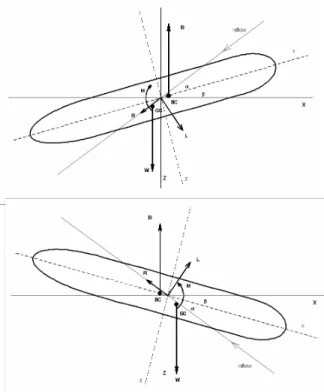
Figure 2(a) shows the hydrodynamic loads which act on a glider during a steady upward glide to the right. Figure 2(b) shows these loads during a steady downward glide to the right.

Figure 2. Definition of Forces and Moments On the Glider Hull (a upper, b lower)

Assume the vehicle is in a steady upward glide with a vehicle pitch angle of beta (β) relative to the horizontal, and, the glide path (trajectory of the GC of the vehicle) is at an angle of gamma (γ) relative to the horizontal. For simplicity, by assuming there is no ocean current affecting the glider then the inflow angle of attack AOA (α) can be easily obtained by subtraction

β γ

(5)

and the vehicle vertical component of speed

w

and horizontal component of speed

u

will satisfy the following relationship.

u/w=tan(α +β) (5) The force and moment equilibrium relations for the vehicle in the XZ plane are

−Rcos(α+β)+Lsin(α+β)=0 (6) −Rsin(α+β)−Lcos(α+β)+B−W =0 (7) 0 ) sin cos ( ) sin cos ( = − + − + M z x W z x B G G B B β β β β (8)

where R, L and M are defined in equations 1 to 3. As the piston of the BE moves, the BC should slide back and forth along the longitudinal centreline of the vehicle. Coordinates (

x

_B,0) and (

x

_G

,

z

_G) indicate the positions for the BC and GC respectively. The standard SNAME sign convention of x positive forward, y positive to starboard and z positive keelward is used throughout this paper.

To initiate an upward glide, Fig 2a, the piston of the BE moves forward to expel the seawater which is within the nose section, and, at the same time the PCW moves aftward. Thus the centre of mass of the piston moves forward while the centre of mass of the PCW moves aftward, and, since the mass of the PCW is greater than the mass of the piston, the effective GC for the vehicle moves aftward, thus during a steady upward glide the GC will be aft of (and below) the origin at (

x

_G

,

z

_G) where

z

_G) where

x

_G and

z

_G will now both be positive quantities. Once the piston of the BE has ingested the maximum volume of seawater into the nose, the volume of

seawater which is displaced by the hull has now decreased so the BC moves aftward of the origin so during a steady downward glide the coordinates of the BC should be (

x

_B,0) where

x

_B is now a negative quantity. During a steady downward glide, the hydrostatic moment (about an axis through the origin) due to the BC being aft of the origin means that the nose will fall. However, at the same time, the de-stabilizing hydrodynamic moment (about an axis through the origin) will cause the nose to rise. Thus during a steady downward glide there must be some pitch attitude of the vehicle where these two counteracting moments are in equilibrium. It is from this equilibrium condition that we can find the value for the hydrodynamic parameter 'd'.

Here W is the dry weight of the glider (in air) and B is the buoyant force which acts on the glider when it is completely submerged.

Both W and B are split into two and three components, (B_h,B_e) and (G_h,G_p,G_e), which are described in the following section.

3 IDENTIFICATION OF PARAMETER d

The method and procedures to estimate the parameters a ,

b and c have been described in the previous article [9]. This paper hereafter will continue todescribe the approach to identify the parameter, d .

z

_Ge) are the gravity centres for the hull, movable battery pack (PCW)and BE respectively.

Substituting Eq. (1, 2, and 3) into Eq. (6, 7, and 8) we obtain

tan(α+β)=CR/CL ε(α) (13) with the definition of ε the ratio of the resistance coefficient over the coefficient of the lift we can find the

(6)

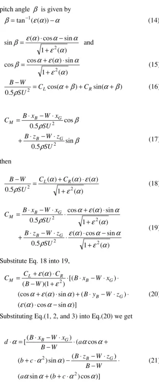
pitch angle β is givenby β=tan−1(ε(α))−α (14) ) ( 1 sin cos ) ( sin 2_α ε α α α ε β + − ⋅ = and ) ( 1 sin ) ( cos cos 2_α ε α α ε α β + ⋅ + = (15) cos( ) sin( ) 5 . 0 ρ 2 = α+β + α+β − R L C C SU W B (16) β ρ β ρ sin 5 . 0 cos 5 . 0 2 2 SU z W z B SU x W x B C G B G B M ⋅ − ⋅ + ⋅ − ⋅ = (17) then ) ( 1 ) ( ) ( ) ( 5 . 0 2 _ε2 _α α ε α α ρ ₊ ⋅ + = − CL CR SU W B (18) ) ( 1 sin cos ) ( 5 . 0 ) ( 1 sin ) ( cos 5 . 0 2 2 2 2 α ε α α α ε ρ α ε α α ε α ρ + − ⋅ ⋅ ⋅ − ⋅ + + ⋅ + ⋅ ⋅ − ⋅ = SU z W z B SU x W x B C G B G B M (19)

Substitute Eq. 18 into 19,

)] sin cos ) ( ( ) ( ) sin ) ( (cos ) [( ) 1 )( ( ) ( 2 α α α ε α α ε α ε α ε − ⋅ ⋅ ⋅ − ⋅ + ⋅ + ⋅ ⋅ − ⋅ ⋅ + − ⋅ + = G B G B R L M z W y B x W x B W B C C C (20)

Substituting Eq.(1, 2, and 3) into Eq.(20) we get

)] cos ) ( sin ( ) ( ) sin ) ( cos ( ) ( [ 2 2 α α α α α α α α α ⋅ + + ⋅ − ⋅ − ⋅ − ⋅ + + ⋅ − ⋅ − ⋅ = ⋅ c b a W B z W z B c b a W B x W x B d G B G B (21)

Using the previously identified parameters a , b and c , and the estimatedpositions of the BC and GC, values for the parameter d were estimated by using equation 21. The positions of the BC and GC were calculated from equations 9 to 12.

The values of Gh , G and b G are determined by e

weighing the individual components; the values of Bh

and Be are determined by suspending the

fully-submerged glider from a single load cell at a point above the BC and GC.

4 DATA FROM AT-SEA EXPERIMENTS

Data collected on-board during experiments at-sea are continuous records or time histories. Only those recorded during steady-state straight-ahead gliding (without rudder deflection) are first selected for further processing. For the present analysis these are the two independently-controlled variables (i) position of the piston for the BE, (ii) position of the PCW, and, the two dependent variables (iii) glider pitch angle 'beta', (iv) depth-sensor reading 'z'. Some of these signals must be pre-processed into intermediate quantities, prior to the parameter identification process. For example, the position of the piston for the BE is used to determine the mass of ballast water which is ingested or expelled by the BE. Another example is the depth-sensor reading since it can be differentiated to give the vertical velocity of the glider. Finally, the net weight (W-B) of the glider when submerged is calculated from the measurement of the piston position relative to its initial position since the initial position corresponds to the level-trim neutrally-buoyant condition.

Voyage 193, from July 2006, provides measured values from 52 descents and ascents to a maximum depth of 190 m. This voyage represents a total of 38 hours in the water. The values used in this analysis are average values computed for each descent and ascent; each ascent and descent was assumed to be in a straight line and to be free of any effects of ocean currents. Typical descents take about 8.9 minutes and typical ascents take about 7.2 minutes. We used an iterative scheme, described in [9], to obtain estimates for the three hydrodynamic parameters (a, b, c) and used the approach presented in section II to estimated the parameter (d). The identified values of these four parameters therefore categorize the gliding behavior in the XZ plane for small angles of attack, −10 < AOA < +10 .

5 RESULTS AND DISCUSSIONS

Figure 3 shows one set of results using the iterative method, as applied to the data from voyage 193. Here the calculated glide path angle is plotted versus the mean of the measured glider pitch angle, for each of the 50 descents and 51 ascents. The data are shown for six categories of glide angle: steep, medium and shallow descents, and, shallow, medium and steep ascents. The 50 dives show glide path angles in the range from 29 to 35 which correspond to glider mean pitch angles of from about −30 to −20 , respectively. Since from (4) the AOA is the difference between the glide path angle and the glider pitch angle, the AOA during descent ranges from about 5 to 9 . Similarly, the 51 ascents show calculated glide path angles in the range from 29 to 35 which correspond to glider mean pitch angles of from about +20 to +30 , respectively, again with the AOA between 5 and 9 .

(7)

Figure 3. Glide path angle vs glider pitch angle Figure 4 shows the corresponding values of the calculated glider speed along the glide path plotted versus the mean measured glider pitch angle. Again the six categories of glides are shown. Here the glide speeds during descent vary from about 39 to 52 cm/s while those during ascents vary from about 42 to 56 cm/s. Clearly the glider was ballasted "light" relative to the surrounding seawater thus the seawater was more dense than the target density used during the pre-voyage ballasting process [8]; this is also corroborated by typical descent and ascent times of 8.9 and 7.2 minutes, respectively.

Figure 4. Glide speed vs glider pitch angle

Figure 5 shows the corresponding values of the estimated AOA plotted versus the estimated glide path angle. Again the six categories of glides are shown. Here it is confirmed that the smallest values of the AOA (approx 5º) occurs with the steepest glide path angles (near 35º), and, from Figure 4 we see that the velocity 'Vo' along the glide path then exceeds 50 cm/s.

Figure 6 shows the corresponding values of the drag coefficient, CD, based on the frontal area, plotted versus

the estimated AOA, for the six categories of glides used

Figure 5. Angle of attack vs glide path angle

in the three previous figures. The data points for the 50 descents form the basis for the upper curve while those for the 51 ascents form the lower curve. Curves of the form given in equation (1) were fitted in order to extract values for the parameters ‘b’ and ‘c’. For glider 049 in the configuration tested, the minimum drag coefficient ‘b’ during descents is expected to be about 0.25 while that for ascents is about 0.19. The curvature parameter ‘c’ is about 6.2 for descents and 6.5 during ascents.

Figure 6. Fitted relations for drag coefficient

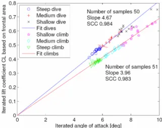
Figure 7 shows the corresponding values of the lift coefficient, CL, based on the frontal area, plotted versus

the estimated AOA, for the six categories of glides used in the previous figures. Again the data points for the 50 descents form the basis for the upper curve while those for the 51 ascents form the lower curve. Straight lines of the form given by equation (2) were fitted. For glider 049 in the configuration tested, the lift curve slope ‘a’ was about 4.7 per degree during descents and was about 4.0 per degree during ascents. The sample correlation coefficient for both cases was about 0.98. Figures 6 and 7 show that

(8)

the calculated angles of attack range from about 5 to 10 during these 101 separate glides of duration from 7 to 9 minutes.

Figure 7. Fitted relations for lift coefficient Figure 8 shows the corresponding values of the parameter 'd' for the pitching moment coefficient, CM, based on the

frontal area and vehicle length, plotted versus the AOA. It appears that there is no single value of 'd' which can be used to represent the hydrodynamic pitching moment variation with AOA, for both dives and climbs. If one calculates a mean value over the range of AOA (-9,-5) for

Figure 8. Identified model parameter d

steady gliding descents and over the range (+5,+9) for ascents, one obtains a mean value for 'd' of 0.57 for dives and 0.49 for climbs. All identified parameters (a, b, c and

d) are summarized in Table 1.

Table 1. Summary of Identified Parameters Parameter Dive Climb

a 4.67 3.96

b 0.25 0.19

c 6.18 6.54

d 0.57 0.49

6 CONCLUSIONS

Our focus at NRC-IOT is on extending theapplications of underwater vehicles with various payload sensors. In this role we add new sensors to ocean gliders. Once a new sensor has been integrated into an existing glider, there is one final step we need to complete before sending the glider on a long-duration mission. We need to categorize the new hydrodynamic behavior of the glider using new data obtained from a set of short-term missions in order to predict the likely duration of a long-term voyage with a new (or fully-charged) battery pack. It is for that purpose that we have completed the development of a new procedure for identifying the four lift, drag and pitching moment parameters (a, b, c, d) as detailed initially in [9] and subsequently in this paper. The fact that each of these four parameters has different values during dives and climbs suggests that there is some geometrical asymmetry in the vertical plane of the glider. For example, the CTD sensor is located below the port wing and the rudder assembly projects well above the hull; these influences required further investigation.

ACKNOWLEDGEMENTS

The authors thank the staff and students at NRC-IOT and Memorial University who have assisted in the preparation of the gliders for the various voyages, and, the various funding agencies which have contributed to the success of this research program. Without their continuing support these measurements, analysis and conclusions would not have been possible.

REFERENCES

[1] Henry Stommel, “The Slocum Mission”,

Oceanography, pp. 22-25, 1989.

[2] Clayton Jones and Doug Webb, “Slocum Gliders, Advancing Oceanography”, in Proceedings of the 15th

International Symposium on Unmanned Untethered Submersible Technology conference (UUST’07), Durham, NH, USA, 19 to 20 Aug 2007. AUSI.

[3] C.C.Eriksen, T.J.Osse, R.D.Light, T.Wen and T.W.Lehman, “Seaglider: A long-range autonomous underwater vehicle for oceanographic research”, IEEE

Journal of Oceanic Engineering, 26:424–436, Oct 2001. [4] J.Sherman, R.E.Davis, W.B.Owens and J.Valdes, “The autonomous underwater glider Spray”, IEEE

Journal of Oceanic Engineering, 26:437–446, Oct 2001. [5] Chunzhao Guo and Naomi Kato,

“

Mini Underwater Glider (MUG) for Education”, in Proceedings of

Workshop for Asian and Pacific Universities' Underwater Roboticians–ApuuRobo, Tokyo, Japan, 13 to 14 Jan 2008. [6] D'Spain, G.L., R. Zimmerman, S.A. Jenkins, J.C. Luby, and P. Brodsky, "Underwater acoustic measurements with a flying wing glider", J. Acoust. Soc.

Am., 121, 3107, 2007.

[7] T. James Osse and Charles C. Eriksen, “The Deepglider: A full ocean depth glider for oceanographic

(9)

research”, in Proceedings of the OCEANS 2007

conference, Vancouver BC, Canada, 01 to 04 Oct 2007. MTS/IEEE.

[8] Ralf Bachmayer, Brad deYoung, Christopher D. Williams, Charlie Bishop, Christian Knapp and Jack Foley, “Development and deployment of ocean gliders on the Newfoundland Shelf”, in Proceedings of the

Unmanned Vehicle Systems Canada Conference 2006, Montebello, Quebec, Canada, 07 to 10 Nov 2006. UVS Canada.

[9] C.D. Williams, R. Bachmayer, and B. deYoung, “Progress in Predicting the Performance of Ocean Gliders from At-Sea Measurements”, in Proceedings of the

OCEANS 2008 Conference, Quebec City, Quebec,

Canada, 15 to 18 Sept 2008. MTS/IEEE.

[10] J.G. Graver, R. Bachmayer, N.E. Leonard, and D.M. Fratantoni, “Underwater glider model parameter identification”, in Proceedings of the 13th International

Symposium on Unmanned Untethered Submersible Technology Conference (UUST’03), Durham, NH, USA, Aug 2003.