Publisher’s version / Version de l'éditeur:
Vous avez des questions? Nous pouvons vous aider. Pour communiquer directement avec un auteur, consultez la Questions? Contact the NRC Publications Archive team at
[email protected]. If you wish to email the authors directly, please see the first page of the publication for their contact information.
https://publications-cnrc.canada.ca/fra/droits
L’accès à ce site Web et l’utilisation de son contenu sont assujettis aux conditions présentées dans le site LISEZ CES CONDITIONS ATTENTIVEMENT AVANT D’UTILISER CE SITE WEB.
International Journal of Hydrogen Energy, 45, 56, pp. 32743-32752, 2020-09-25
READ THESE TERMS AND CONDITIONS CAREFULLY BEFORE USING THIS WEBSITE. https://nrc-publications.canada.ca/eng/copyright
NRC Publications Archive Record / Notice des Archives des publications du CNRC : https://nrc-publications.canada.ca/eng/view/object/?id=fb5f533f-5158-424f-8c22-432e6d85cec3 https://publications-cnrc.canada.ca/fra/voir/objet/?id=fb5f533f-5158-424f-8c22-432e6d85cec3
NRC Publications Archive
Archives des publications du CNRC
This publication could be one of several versions: author’s original, accepted manuscript or the publisher’s version. / La version de cette publication peut être l’une des suivantes : la version prépublication de l’auteur, la version acceptée du manuscrit ou la version de l’éditeur.
For the publisher’s version, please access the DOI link below./ Pour consulter la version de l’éditeur, utilisez le lien DOI ci-dessous.
https://doi.org/10.1016/j.ijhydene.2020.08.281
Access and use of this website and the material on it are subject to the Terms and Conditions set forth at
Predicting fueling process on hydrogen refueling stations using
multi-task machine learning
Graphical Abstract
Predicting Fueling Process on Hydrogen Refueling Stations using Multi-Task Machine Learning
Highlights
Predicting Fueling Process on Hydrogen Refueling Stations using Multi-Task Machine Learning
Yunli Wang1, Cyrille Dec`es-Petit2
• Machine learning methods for classification and prediction of the fueling process.
• Classifying fueling events reached over 85% accuracy on three stations. • Multi-task machine learning models predicted state of charge
accu-rately.
• Models from rich stations improved the prediction on the data-poor station.
Predicting Fueling Process on Hydrogen Refueling
Stations using Multi-Task Machine Learning
Yunli Wang1∗, Cyrille Dec`es-Petit2 1 Digital Technologies Research Centre
National Research Council Canada 1200 Montreal Road Ottawa, ON, Canada K1A 0R6
2 Energy, Mining and Environment Research Centre National Research Council Canada
4250 Wesbrook Mall Vancouver, BC, Canada V6T 1W5
Abstract
Monitoring hydrogen refueling stations (HRS) ensures the safety of their op-erations as well as meeting the required performance standard for refueling. Traditionally, table-based or dynamic control of fueling process methods were used to guide the fueling process. We propose to use machine learning meth-ods to predict the main performance target of the fueling process; the state of charge (SOC). Based on initial operating conditions in start-up fueling time, least absolute shrinkage and selection operator (LASSO) is used to predict non-dispensing fueling events, normal, and undershot dispensing events. The computational experiments were conducted on three hydrogen refueling sta-tions with up to two-years of operational data. The classification accuracy reached over 85% on three stations. The SOC in future time steps were pre-dicted using a multi-task regression model. The prepre-dicted future SOC within one minute is accurate on two data-rich stations. In both classification and regression tasks, the training models built on data-rich stations greatly im-proved the performance of a station with much less training data. These results show using machine learning methods on predicting the performance of fueling events is feasible and satisfactory on HRS. To optimize operation
∗Corresponding author
Email addresses: [email protected] (Yunli Wang1), [email protected] (Cyrille Dec`es-Petit2)
strategies, machine learning models can be integrated into the controller of HRS as an alternative way of controlling the fueling process.
Keywords: Hydrogen Refueling Station, Machine Learning, Multi-task Learning
1. Introduction
The electrification of transportation has been widely accepted as an effi-cient means of reducing carbon emission. In the past 20 years, advances in hydrogen fuel cells have enabled the electrification of transportation thanks to a significant increase in energy density by weight and volume. Networks of hydrogen refueling stations (HRS) are being developed across Canada and in many other countries. With the increase of hydrogen refueling infrastruc-ture, monitoring these hydrogen refueling stations ensures the safety of their operations.
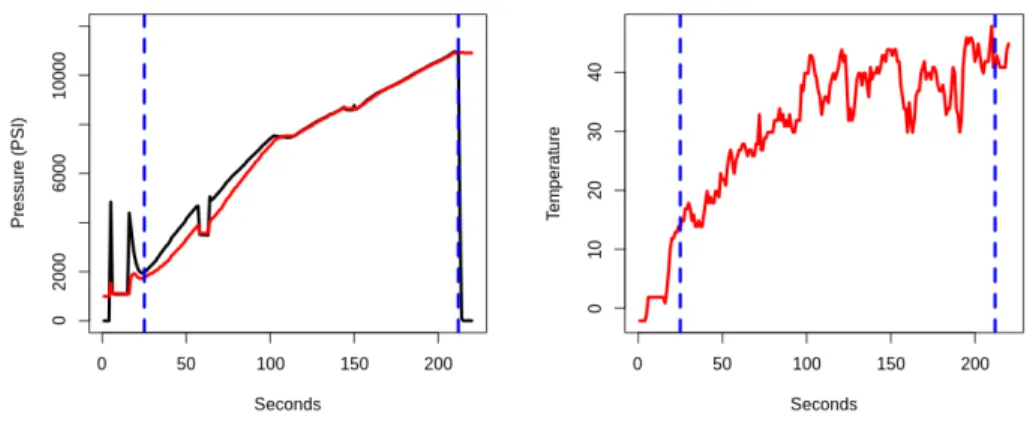
A hydrogen refueling station is typically composed of a compressor, stor-age banks, controller, chiller, and dispenser. As defined in the Fueling Pro-tocols for Light Duty Gaseous Hydrogen Surface Vehicles SAE J2601, the fueling process consists of a start-up time, main fueling time, and shutdown time [1]. A representative fueling profile is shown in Figure 1. During start-up time (left of the first vertical blue line), the nozzle is connected to the vehicle, and a connection pulse is initiated consisting of a brief increase and hold of pressure. The station measures the initial pressure and the capacity category of the compressed hydrogen storage system (CHSS) of the vehicle in this start-up time. The initial leak check is performed after the nozzle is connected and prior to the main fueling time. If the dispenser is properly connected to the vehicle and there is no pressure decay indicating a leak, the main fueling begins with the hydrogen flowing into the vehicle tank. During the main fueling time (between two vertical blue lines), the pressure rises and the temperature of CHSS increases. At most two leak checks are performed during the main fueling time to determine if there are any leaks in the system. The CHSS capacity determined during the start-up time is used to determine the State of Charge (SOC). SOC is the ratio of CHSS hydrogen density to the density at Normal Working Pressure (NWP) rated at the standard tem-perature 15oC [1]. When SOC is above 95% (it can be either the station or
the CHSS SOC, whichever is greater), the hydrogen stops being dispensed to the vehicle. In this shutdown phase (right of the second vertical blue line),
the hydrogen in the dispenser hose is vented to release the pressure in the line.
Figure 1: A representative fueling profile, left panel: station pressure (black) and vehicle pressure (red); right panel: vehicle temperature.
In this study, the following terms are used and defined to analyse the HRS dispensing operation:
Fueling event: a fueling process including at least start-up time after the nozzle is connected to the vehicle, and also main fueling time and shutdown time if fueling continues.
Dispensing event: a fueling event includes the period when the hydrogen is dispensed to the vehicle.
Normal dispensing event: a dispensing event in which the SOC reaches 95% and less than 100% at the end of fueling.
Overshot dispensing event: when the vehicle SOC or the station SOC is over 100% at any time during a dispensing event.
Undershot dispensing event: the vehicle SOC or the station SOC is under 95% at the end of the dispensing event.
The fueling process in hydrogen refueling stations is a complex process. Both experimental and analytical studies using simulation models or ther-modynamic models have been conducted to inspect key parameters of the
fueling process. The effect of the initial tank temperature, tank properties, inlet temperature, ambient temperature on the fueling process parameters in-cluding the SOC, final temperature, final pressure and cooling demand have been examined. Earlier experimental studies focus on temperature rise dur-ing the refueldur-ing process [2, 3, 4, 5]. Computational fluid dynamics models [6, 7, 8], and analytical thermodynamics models have been used to study the evolution of the hydrogen temperature and pressure during fast filling [9, 10]. Simulation models of refueling station components have also been devel-oped to optimize station compression and storage. Some studies target the refueling station configurations [11, 12] to improve the fueling and reduce en-ergy consumption [13, 14]. Other studies focus on fast fueling since shorter fueling time reduces the amount of energy consumption [9, 15], but fast fuel-ing leads to a temperature rise [3]. The safe and fast fillfuel-ing strategies based on the analytical models in numerical studies were summarized [15].
Several studies used the analytical solution of thermodynamic models to predict the temperature change and final temperature in the hydrogen refueling process [16, 17, 18, 19, 20, 21]. Although the parameter estimated from thermodynamic models matched with the simulated models, only a limited number of factors can be considered in those models.
Many studies have investigated the optimization of the hydrogen filling process. Zeng et al. proposed a multi-objective iterative optimization model for a three-stage refueling process and an optimization algorithm for the filling process [22]. Since the release of SAE J2601, methods using table-based or formula table-based on total heat capacity (MC formula) are often used to optimize the operation strategies and control the fueling process [1]. These two methods were compared, and the MC formula method greatly reduces the fueling time since it takes advantage of the active measurement of the precooling temperature to dynamically control the fueling process [9]. Kuroki et al. utilized a dynamic simulation model to estimate the key parameters during the refueling process [23]. On top of the dynamic simulation, Chae et al. developed a thermodynamic model for real-time responding hydrogen fueling protocol using real-time simulation and real-time data [24].
We propose to use machine learning methods for monitoring the fueling process and predicting the SOC value by measuring the temperature and pressure of all components. Machine learning models have been used to monitor the health of equipment, diagnosis, prognosis, and fault detection in many applications [25, 26, 27, 28, 29]. To our knowledge, machine learning methods have not been used to predict the outcomes of the fueling process to
optimize operation strategies. SOC is directly related to temperatures and pressures in the CHSS of the vehicle as well as in the HRS. Many other factors also affect the SOC and the completion of the fueling process, such as the communication between car and station, the operation of the high pressure storage, and the operation of the compressor etc. In other studies using simulation models or analytical thermodynamic models, only a few factors that influence SOC or other key performance parameters can be considered. The machine learning model we propose can include all available sensor values from HRS, and automatically choose important attributes that contribute to SOC and also capture the dynamic change of temperature and pressure during the filling process.
In this study, we collected large amounts of sensor data from three hy-drogen refueling stations of type H70-T40 with different time spans and built prediction models to predict the outcomes of the fueling events. We applied a classification model to classify the categories of the fueling process using the initial operating conditions. Moreover, we formulated predicting SOC in several future time slots as a multi-task learning problem. The prediction model can be used to guide the fueling process, for example, terminating non-dispensing events early to save energy or adopting top-off fueling to improve the normal dispensing rate.
2. Methods
In this section, we introduce least absolute shrinkage and selection opera-tor (LASSO) and multi-response LASSO, and then apply LASSO for variable selection, classification and regression tasks. Many factors are associated with SOC, and the main attributes associated with SOC can be identified from variable selection using LASSO. LASSO is used for classifying the cate-gories of fueling events based on all attributes. Also, multi-response LASSO is utilized as a multi-task regression model to predict SOC in the future time steps.
2.1. Least Absolute Shrinkage and Selection Operator
Given data (X, y), X = (X1, X2, X3, ..., Xm) and y are the predictors and
response with N samples and M attributes. For a typical linear regression problem y = β0+ Xβ, the ordinary least squares estimates are obtained by
minimized squared error. argmin N X i=1 (yi− β0 − X j βjxij)2 (1)
LASSO shrinks some coefficients and sets others to 0, and retains the good features of both subset selection [30]. The objective function of LASSO is: min(β0, β) 1 2N N X i=1 kyi − β0− xiβk2F + m X j=1 kβjk1 (2)
The prior knowledge can be incorporated into LASSO using penalty factor p for each attribute Xj. Let pj ∈ [0, 1] be the penalty factor for Xj. If there
is strong evidence a Xj is related to Y , a small penalty or no penalty pj = 0
can be set for Xj. Otherwise, we can set pj = 0.5 if some evidence is derived
from prior knowledge. The generalized objective function of LASSO with penalty factor is represented as:
min(β0, β) 1 2N N X i=1 ky − β0− xiβk2F + m X j=1 pj[(1 − α)kβjk22+ αkβjk1] (3)
α is the elastic-net penalty, which is set to get a linear combination of kβjk1 and kβjk2. From this equation 3, we can derive three models: LASSO
(α = 1), ridge (α = 0) and elastic net(α = 0.5). Since we are interested in a small set of predictors in the regression model, LASSO (α = 1) is exclusively used in this paper.
2.2. Multi-response LASSO
As an extension of LASSO to multiple responses, LASSOm [31] is used as the multiple-response linear regression model. Consider K response Y = (Y1, Y2, ..., Yk) ∈ RN ×K for N samples, a linear regression model from X ∈
RN ×M to Y is given as: Y = β
0+ Xβ, Where β0 is a vector, β ∈ RM ×K is a
coefficient matrix.
The objective function of LASSOm is:
min(β0, β) 1 2N N X i=1 kY − β0− xiβk2F + m X j=1 kβjk1 (4)
2.3. Variable selection using LASSO
A fueling event can be represented as a multivariate time series data with X in N time steps and M attributes, and SOC as y. LASSO is used to identify major attributes that are associated with SOC since it sets the coefficient of many attributes to 0 (Equation 2). By fitting a regression model, a group of attributes with minimized error can be identified from Equation 2.
To illustrate the model selection in LASSO, we use HRS fueling data for demonstration. All attributes are analyzed using LASSO and the factors that associated with SOC are identified based on predictors in the regression model with minimized prediction errors (Figure 2). With the increase in the number of predictors (labels on the top) in the model, mean-squared error (MSE) decreases until it flattens. In Figure 2, the left vertical line locates the model (Mmin) with minimized MSE including around 107 predictors, while
the right vertical line pinpoints to another model (M1se) of which the error
is within one standard error of Mmin. M1se model corresponds to only more
than 60 predictors. In our study, M1se is used to reduce the number of main
attributes identified.
2.4. Classifying fueling events
As described in Introduction, fueling event is a categorical variable. Pre-dicting the categories of fueling events is formulated as binary classification or multi-class classification. In binary classification, fueling events is catego-rized into dispensing 1 or non-dispensing 0. Dispensing events fall into three categories: normal, undershot or overshot. Since the overshot fueling events are rare, dispensing events are classified into normal 1 or undershot 0. For all fueling events, multi-class classification is performed based on the categories of non-dispensing, normal and undershot.
LASSO fits a generalized linear regression model, and the distribution of response variable can be Gaussian, multi-Gaussian, binomial, or multino-mial. In the logistic regression model, response variable follows a binomial or multinomial distribution. For binary classification, y is a Bernoulli dis-tribution, which is a special case of the binomial distribution. Supposing the response variable y takes values in g ∈ 0, 1, the logistic model is repre-sented as logP r(g=1|X=x)P r(g=0|X=x) = β0+ βTX. The objective function for the logistic
regression uses the negative binomial log-likelihood:
min(β0, β) − [ 1 N N X i=1 yi˙(β0+ XiTβ) − log(1 + e β0+XiTβ)] + m X j=1 pjkβjk1 (5)
In multi-class classification, y is a categorical distribution with g out-comes. The probability mass function of y is f (y = i|p) = pri, where
p = (pr1, .., prg). pri is the probability of i,
Pg
i=1pri = 1.
For either binary or multi-class classification, multiple time steps sensor values during start-up fueling time are used to predict the categories of final SOC. It is expected that the prediction becomes more accurate with the increase in number of time steps T .
2.5. Forecasting SOC using multi-task learning
We aim to forecast SOC in future time steps to guide the fueling process. The SOC values in future time steps are correlated, so we formulate predict-ing SOC in several time steps as a multi-task learnpredict-ing problem. Multi-task learning aims to improve the learning of a model by using the information in multiple related tasks [32]. In variable selection, SOC is considered as a Gaussian distribution in the LASSO regression model. In multi-task learn-ing, multiple SOC values follows a multi-Gaussian distribution. Specifically,
we predict multiple SOC values in the future as Y in the multi-response LASSO regression model. Y is k dimensional multi-Gaussian distribution Y = (Y1, ..., Yk), Y ∼ N (µ, σ). LASSOm fits the multi-response model to
select a group of attributes that minimize multiple predicted SOC (Equation 4).
3. Results 3.1. Datasets
Fueling datasets from S1, S2 and S3 were collected from three stations (Table 1). Fueling data records analogic, digital and computed values at about every second during fueling events. The amount of data available for three stations varies. S1 had infrequent fueling events and a small amount of data. S2 provided over one and a half years of data with the largest number of fueling events. Although S3 only had six months of data, the fueling events on it were more frequent. S2 and S3 are considered data-rich stations.
Table 1: Description of fueling datasets collected from S1, S2 and S3.
Station Start End Items Attributes
S1 June 2017 December 2017 1108 154
S2 August 2018 February 2020 99437 166
S3 January 2019 June 2019 28776 186
3.2. Evaluation
In this study, LASSO is used as a regression or a classification model. All experiments were performed on five-fold cross validation. In the regression model for predicting SOC, Root Mean Squared Error (RMSE) is used to measure the difference between predicted SOC and true SOC. Accuracy is used to measure the performance of binary and multi-class classification. In binary classification between dispensing and non-dispensing events, the ac-curacy shows the percentage of true predicted dispensing and non-dispensing events among all fueling events. For classification between normal and un-dershot dispensing, the accuracy describes the predicted true normal and undershot among all dispensing events. In multi-class classification, the ac-curacy indicates the overall performance of classifying fueling events into non-dispensing, normal, or undershot dispensing.
3.3. Variable selection
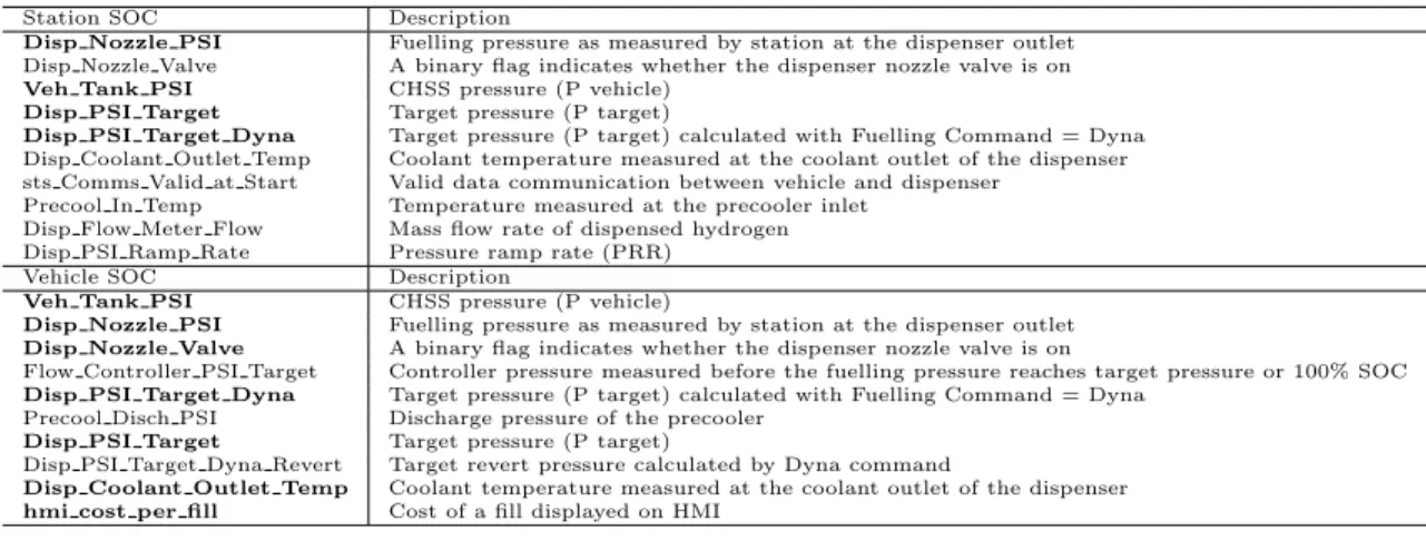
We fit regression models on all fueling events and selected major at-tributes associated with SOC on S2. The top 10 most frequent atat-tributes associated with station SOC or vehicle SOC respectively on S2 are shown in Table 2. As expected, the fueling pressure measured at the dispenser outlet and CHSS pressure are main factors associated with SOC. Other pressure related attributes such as target dispenser pressure and temperature related attributes such as coolant temperature are identified as well. At the same time, sensors indicating valid communication between the vehicle and the station appear as major factors. The results of variable selection on S1 and S3 are similar to that of S2 (data not shown).
Table 2: Major factors associated with station and vehicle SOC on S2.
Station SOC Description
Disp Nozzle PSI Fuelling pressure as measured by station at the dispenser outlet Disp Nozzle Valve A binary flag indicates whether the dispenser nozzle valve is on Veh Tank PSI CHSS pressure (P vehicle)
Disp PSI Target Target pressure (P target)
Disp PSI Target Dyna Target pressure (P target) calculated with Fuelling Command = Dyna Disp Coolant Outlet Temp Coolant temperature measured at the coolant outlet of the dispenser sts Comms Valid at Start Valid data communication between vehicle and dispenser
Precool In Temp Temperature measured at the precooler inlet Disp Flow Meter Flow Mass flow rate of dispensed hydrogen Disp PSI Ramp Rate Pressure ramp rate (PRR)
Vehicle SOC Description
Veh Tank PSI CHSS pressure (P vehicle)
Disp Nozzle PSI Fuelling pressure as measured by station at the dispenser outlet Disp Nozzle Valve A binary flag indicates whether the dispenser nozzle valve is on
Flow Controller PSI Target Controller pressure measured before the fuelling pressure reaches target pressure or 100% SOC Disp PSI Target Dyna Target pressure (P target) calculated with Fuelling Command = Dyna
Precool Disch PSI Discharge pressure of the precooler Disp PSI Target Target pressure (P target)
Disp PSI Target Dyna Revert Target revert pressure calculated by Dyna command
Disp Coolant Outlet Temp Coolant temperature measured at the coolant outlet of the dispenser hmi cost per fill Cost of a fill displayed on HMI
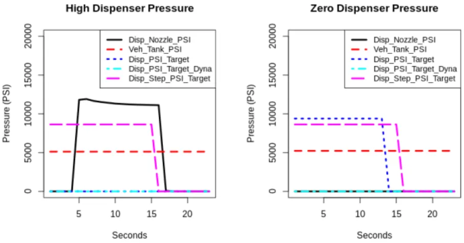
The variable selection is also performed on a subset of fueling data to choose the attributes that are unique to a certain stage of fueling. In the fueling data, each time step is also labeled with a fueling stage, and higher stages represent higher SOC. The start-up fueling time includes stages from 0 to 3, the main fueling time are labeled with stages from 4 to 13, and the shut-down time ends with stage 15. A HRS uses valves to control the open, close, and switch of low, medium, and high storage banks during the fueling process. The valve controlling the flow from one of the storage banks to the dispenser is open during the dispensing process. Six main attributes identified from variable selection in stages 3 and 4 are shown in Figure 3. These two plots show two scenarios of non-dispensing events: one with high
dispenser pressure (left) and another with zero dispenser pressure (right). Zero dispenser pressure indicates the valve did not open and high dispenser pressure was caused by the fact that the station and the vehicle were not properly connected. Variable selection is beneficial for us to understand how the HRS system works, which variables contribute to the performance of HRS, and which variables that can be used to improve the performance.
Figure 3: Factors associated with fueling events in stage 3.
3.4. Classification
Classification models are utilized to predict the outcomes of fueling events based on initial sensor values in start-up and main fueling time. Also, the experiments of using models from data-rich stations to improve the prediction on a data-poor HRS are conducted.
3.4.1. Classification of abnormal fueling events
In the experiments of binary and multi-class classifications, we used all attributes in start-up and main fueling time to predict the categories of final SOC. The attributes of multiple time steps in initial 3, 4, 5, 10, 15, 20 seconds were utilized. The classification accuracy of binary and multi-class classifications are shown in Table 3.
The results of classifying non-dispensing and dispensing fueling events show that accuracy increases with more time steps. It is expected that the classification accuracy is improved by using more information (sensor values) in the initial stage of fueling. On S1, the accuracy obviously jumps with some
fluctuation using 5 or more time steps. The overall performance of S1 is much lower than that of S2 and S3 since it has a small training data. On S2 and S3, the overall performance reaches over 90% using three-second data, and the improvement on more time steps is trivial. It indicates that the classification models can reliably separate non-dispensing and dispensing events based on three seconds of sensor data on S2 and S3.
Classifying normal and undershot dispensing events presents similar re-sults. The performance of S1 is very low, S2 reaches close to 80%, and S3 achieves 88%. The accuracy on S1 drops with more time steps. Conversely, the performance on S2 and S3 improves slightly with more time steps. The accuracy of using three-second time steps is comparable to more time steps on S2 and S3, so using a small amount of sensor data is sufficient to iden-tify undershot on these two stations. The accuracy of splitting normal and undershot on three HRS is lower than that of classifying non-dispensing and dispensing. It shows this task is more challenging since it used the initial sensor values to predict the final SOC. The profiles of normal and undershot dispensing events are similar especially at the initial start-up time, and they differ more at the later stage of fueling.
Multi-class classification aims to determine non-dispensing, normal, and undershot using sensor data at the beginning of the fueling process. The performance on three stations improves with more time steps. It reaches over 80% on S2 and S3, but still performs poorly on S1. Using more than five-second time steps on S2 is effective, but seems unnecessary on S3.
Table 3: Classification accuracy on three stations. Classification Time Steps(s) S1 S2 S3
3 0.640 0.957 0.908 Dispensing 4 0.640 0.957 0.917 vs 5 0.773 0.959 0.920 Non-dispensing 10 0.733 0.961 0.957 15 0.675 0.957 0.950 20 0.861 0.965 0.937 3 0.448 0.783 0.857 Normal 4 0.447 0.799 0.882 vs 5 0.139 0.788 0.862 Undershot 10 0.338 0.785 0.861 15 0.338 0.793 0.861 20 0.139 0.790 0.870 3 0.501 0.676 0.825 4 0.360 0.676 0.794 Multi-class 5 0.440 0.808 0.844 10 0.670 0.801 0.840 15 0.473 0.811 0.847 20 0.697 0.798 0.852
3.4.2. Cold-start classification of abnormal fueling events
Although classification models reach adequate results on S2 and S3, the performance on S1 is low since its training data is limited. The dispenser category of S1, S2, and S3 is the same type of H70-T40. Therefore, a clas-sification model can be trained on S2 and/or S3, and tested on S1. At first, a new dataset with common attributes is extracted on each station, so the number of common attributes is reduced to 229. Then, a baseline classifica-tion model is trained using S1 data and tested on S1. The baseline model shows the performance of using training data on the local station. Lastly, new models are trained on S2 and/or S3 data, but tested on S1. These new models show whether using training data from data-rich stations will improve the prediction on the local station. The classification results are shown in Table 4.
On two binary classification tasks, new models (trained on S2 and/or S3 and tested on S1) outperform the baseline models, while the new models only
perform better on more than four-second time steps in the multi-class classi-fication. New models do not use any S1 training data, and the performance of these models is superior. It demonstrates that without any training data from a new HRS, a prediction model built on other stations can be exploited. Another interesting discovery is the prediction accuracy of new models using three or four second sensor data is higher than using more time steps on two binary classification tasks. This indicates that the initial operating condition represented by three or four second sensor data is sufficient to capture the factors that separate dispensing and non-dispensing events or normal and undershot dispensing events.
Table 4: Classification accuracy using data from other stations. Train Time Steps S1 S2 S3 S2 & S3
Test (s) S1 S1 S1 S1 3 0.653 0.467 0.600 0.680 Dispensing 4 0.693 0.227 0.760 0.827 vs 5 0.640 0.333 0.800 0.840 Non-dispensing 10 0.773 0.787 0.880 0.827 15 0.817 0.750 0.889 0.847 20 0.601 0.819 0.861 0.847 3 0.417 0.140 0.386 0.772 Normal 4 0.274 0.825 0.281 0.702 vs 5 0.285 0.825 0.281 0.719 Undershot 10 0.286 0.754 0.596 0.702 15 0.338 0.789 0.491 0.702 20 0.141 0.596 0.509 0.754 3 0.585 0.333 0.387 0.453 4 0.659 0.400 0.427 0.533 Multi-class 5 0.599 0.493 0.520 0.653 10 0.581 0.533 0.560 0.587 15 0.589 0.556 0.625 0.625 20 0.576 0.569 0.625 0.542 3.5. Regression
In experiments of predicting SOC, the results of using the regression model on sensor values in the current single time step are presented first.
This is followed by forecasting SOC in several future time steps as multi-task leaning. Lastly, improvement of a data-poor station using the regression models trained on data-rich stations is described.
3.5.1. Predicting SOC using LASSO
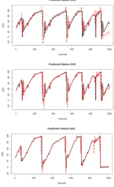
In Section 3.3, a regression model is fit using LASSO to identify major attributes associated with SOC, and this model can also be used to predict SOC using the station SOC or vehicle SOC as the target response variables. All attributes in current time step T 0 or merged with previous time steps in P T 1 ∼ P T 5 are used to predict SOC. The results on S2 show that the performance of just using the current time step is low, and is much improved when combined with previous time steps (Table 5). Figure 4 shows a segment of the predicted SOC (red) and true SOC (black). The gap between the predicted SOC and station SOC is larger using the current time step than the merged time steps. The prediction is more accurate on vehicle SOC; however, using attributes from more than one time steps only slightly reduced the prediction error (Table 5).
Table 5: RMSE of predicted station and vehicle SOC on S2. Knowledge Time Steps Station SOC Vehicle SOC
T0 12.20 9.63 PT1∼T0 6.47 4.82 PT2∼T0 6.25 4.81 No PT3∼T0 6.23 4.78 PT4∼T0 6.19 4.76 PT5∼T0 6.19 4.74 Yes T0 12.16 9.61
In addition, the experiment of using prior knowledge to predict SOC was also performed. SOC is directly related to dispenser pressure and vehicle tank pressure, so these two attributes are used as prior knowledge. The penalty factors for these two attributes are set as 0 in the linear regression model of LASSO (Equation 3). RMSE of predicted station SOC and vehicle SOC using the current time step (the last row in Table 5) are very close to the model without prior knowledge (the first row in Table 5). Using prior knowledge does not have a big impact on predicting SOC due to its
Figure 4: A segment of predicted SOC (red) and true SOC (black), top: predicted station SOC using the current time step; middle: predicted station SOC using the current and one previous time steps; bottom: predicted vehicle SOC using the current and one previous time steps.
association with many other attributes. As shown in Figure 2, more than 60 attributes exist in the regression model M1se.
3.5.2. Multi-task learning for predicting SOC
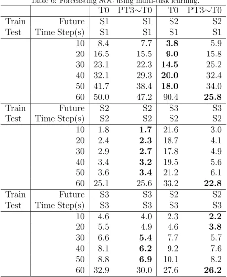
Predicting SOC in future time steps is considered a multi-task learning problem. SOC at the following 10, 20, 30, 40, 50 and 60 seconds were pre-dicted using LASSOm on the sensor values in current time step T 0 as well as the previous three time steps P T 3 ∼ P T 1. The results of multi-task learning for predicting SOC are described in the third column in Table 6. As expected, the RMSE of predicted SOC gradually gets worse with the increase of gap between the current and future time steps. RMSE on S2 and on S3 are quite low, while the prediction error is high on S1. On all three stations, the prediction is worst when predicting SOC at 60 seconds. Using multiple time steps, the prediction error is slightly reduced.
The performance of regression models depends upon the amount of avail-able training data. Since predicting future SOC is a difficult task on three stations, the performance of using models from other stations is tested. The results are shown in the fourth column in Table 6. The baseline models were built on one station and tested on that station (Third Column); while new models were built on another station, but tested on the current station (Fourth Column). On S1, the model trained on S2 outperforms the base-line model trained on S1. The performance of predicting SOC on S2 already reached low RMSE, so the model trained on S3 does not surpass the baseline. On S3, models trained on S2 boosted the performance of SOC prediction at 10, 20 and 60 seconds. Using new models on multiple time steps had limited success to predict SOC at the 10, 20, and 60 seconds compared with a single time step.
Table 6: Forecasting SOC using multi-task learning. T0 PT3∼T0 T0 PT3∼T0
Train Future S1 S1 S2 S2
Test Time Step(s) S1 S1 S1 S1
10 8.4 7.7 3.8 5.9 20 16.5 15.5 9.0 15.8 30 23.1 22.3 14.5 25.2 40 32.1 29.3 20.0 32.4 50 41.7 38.4 18.0 34.0 60 50.0 47.2 90.4 25.8 Train Future S2 S2 S3 S3
Test Time Step(s) S2 S2 S2 S2
10 1.8 1.7 21.6 3.0 20 2.4 2.3 18.7 4.1 30 2.9 2.7 17.8 4.9 40 3.4 3.2 19.5 5.6 50 3.6 3.4 21.2 6.1 60 25.1 25.6 33.2 22.8 Train Future S3 S3 S2 S2
Test Time Step(s) S3 S3 S3 S3
10 4.6 4.0 2.3 2.2 20 5.5 4.9 4.6 3.8 30 6.6 5.4 7.7 5.7 40 8.1 6.2 9.2 7.6 50 8.8 6.9 10.1 8.2 60 32.9 30.0 27.6 26.2 4. Discussion
This paper proposes to predict the performance of fueling events using the machine learning model LASSO. It is used for variable selection, classi-fication, and regression. LASSO has been widely used in many applications for its effectiveness and efficiency in identifying major factors [27, 28, 29]. LASSO was one of the main methods used for variable selection in many process control applications reviewed in [27]. We also tested other machine learning models such as XGBoost [33] in classification and regression tasks.
The performance of XGBoost is comparable to LASSO. The main purpose of this study is not to compare the performance of different machine learning approaches, but to promote applying machine learning methods in predict-ing the performance of fuelpredict-ing processes and incorporatpredict-ing machine learnpredict-ing models into control systems of HRS in the future.
Multi-task learning for SOC forecasting reached reasonable performance within one minute. Usually a normal fueling process lasts over three minutes, so it is desirable to predict the final SOC using the initial sensor values. The performance of predicting SOC has deteriorated at 60 seconds, so predicting the final SOC will be much more challenging.
5. Conclusions
This study proposes using the machine learning model LASSO for classi-fying non-dispensing, normal or undershot dispensing events based on initial operating conditions, and forecasting SOC in future time steps in on-line monitoring scenarios.
Fueling data was collected from three stations: S1, S2 and S3, but only small amounts of data were available on S1. LASSO was able to identify vari-ables associated with SOC on HRS. Fueling events fall into non-dispensing, normal and undershot dispensing categories. In binary classification tasks of between non-dispensing and dispensing, and between normal and undershot dispensing, LASSO reached over 85% accuracy on S2 and S3, and the per-formance of S1 was improved by using the prediction models of S2 and/or S3. The results indicates the machine learning method can reliably predict fueling events even on a new HRS.
Multi-task regression models are proposed for SOC forecasting. The mul-tiple co-related future SOC are considered in the regression model. Forecast-ing SOC at subsequent 10, 20, 30, 40, and 50 seconds reached satisfactory results on S2 and S3, but performed poorly on S1. Using training data from other stations greatly improved the performance on S1. Using prediction models from other stations it is possible to transfer the knowledge from oth-ers to a new HRS. This mechanism enables the experience gained over the operation of the first several stations to benefit the operation of new stations. If the machine learning method is integrated in the controller of HRS, the prediction models can be used for optimizing operation strategies. Ad-ditionally, the models can be incrementally updated with new data, and the performance would improved overtime with more training data. Predicting
the outcomes of fueling event based on the first several seconds of sensor data using classification models can be used to activate some fueling procedures such as top-off fueling. Forecasting SOC in future time steps using regres-sion models is suitable for real-time monitoring fueling processes to ensure the safe operation of HRS.
This work focused on predicting SOC in the fueling process. Predicting the final SOC in the subsequent three minutes is a realistic but challenging problem. More studies are needed to examine the effect of dynamic opera-tional conditions on other parameters such as the final temperature and final pressure using prediction models. Other prediction models besides LASSO estimating the non-linear relationship between the evolution of temperature and pressure in fueling process and filling time, or ultimately, energy con-sumption, will be explored in the future. We advocate adopting machine learning methods to improve the performance of HRS. With the increase in commercial operation of HRS and growth of hydrogen refuelling infrastruc-ture, highly efficient and reliable HRS are needed to promote more clean energy.
Acknowledgements
This project was supported by Transport Canada. The authors would like to thank Kathy Kneale and Aaron Conde for their help to improve the manuscript.
References
[1] J. Schneider, SAE J2601-worldwide hydrogen fueling protocol: Status, standardization & implementation, SAE Fuel Cell Interface. nd Accessed 12 (2014).
[2] C. Dicken, W. M´erida, Temperature distribution within a compressed gas cylinder during fast filling, in: Advanced materials research, Vol. 15, Trans Tech Publ, 2007, pp. 281–286.
[3] C. Dicken, W. Merida, Measured effects of filling time and initial mass on the temperature distribution within a hydrogen cylinder during re-fuelling, Journal of Power Sources 165 (1) (2007) 324–336.
[4] Y.-L. Liu, Y.-Z. Zhao, L. Zhao, X. Li, H.-g. Chen, L.-F. Zhang, H. Zhao, R.-H. Sheng, T. Xie, D.-H. Hu, et al., Experimental studies on tem-perature rise within a hydrogen cylinder during refueling, International Journal of Hydrogen Energy 35 (7) (2010) 2627–2632.
[5] R. O. Cebolla, B. Acosta, P. Moretto, N. Frischauf, F. Harskamp, C. Bonato, D. Baraldi, Hydrogen tank first filling experiments at the JRC-IET GasTeF facility, International Journal of Hydrogen Energy 39 (11) (2014) 6261–6267.
[6] M. C. Galassi, D. Baraldi, B. A. Iborra, P. Moretto, CFD analysis of fast filling scenarios for 70 MPa hydrogen type IV tanks, International Journal of Hydrogen Energy 37 (8) (2012) 6886–6892.
[7] M. C. Galassi, E. Papanikolaou, M. Heitsch, D. Baraldi, B. A. Iborra, P. Moretto, Assessment of CFD models for hydrogen fast filling simu-lations, International Journal of Hydrogen Energy 39 (11) (2014) 6252– 6260.
[8] D. Melideo, D. Baraldi, CFD analysis of fast filling strategies for hydro-gen tanks and their effects on key-parameters, International Journal of Hydrogen Energy 40 (1) (2015) 735–745.
[9] K. Reddi, A. Elgowainy, N. Rustagi, E. Gupta, Impact of hydrogen SAE J2601 fueling methods on fueling time of light-duty fuel cell elec-tric vehicles, International Journal of Hydrogen Energy 42 (26) (2017) 16675–16685.
[10] E. Rothuizen, B. Elmegaard, M. Rokni, Dynamic simulation of the effect of vehicle-side pressure loss of hydrogen fueling process, International Journal of Hydrogen Energy 45 (15) (2020) 9025–9038.
[11] J. Zheng, X. Liu, P. Xu, P. Liu, Y. Zhao, J. Yang, Development of high pressure gaseous hydrogen storage technologies, International Journal of Hydrogen Energy 37 (1) (2012) 1048–1057.
[12] K. Reddi, A. Elgowainy, E. Sutherland, Hydrogen refueling station com-pression and storage optimization with tube-trailer deliveries, Interna-tional Journal of Hydrogen Energy 39 (33) (2014) 19169–19181.
[13] J. Guo, L. Xing, Z. Hua, C. Gu, J. Zheng, Optimization of compressed hydrogen gas cycling test system based on multi-stage storage and self-pressurized method, International Journal of Hydrogen Energy 41 (36) (2016) 16306–16315.
[14] A. Bauer, T. Mayer, M. Semmel, M. A. G. Morales, J. Wind, Energetic evaluation of hydrogen refueling stations with liquid or gaseous stored hydrogen, International Journal of Hydrogen Energy 44 (13) (2019) 6795 – 6812.
[15] M. Li, Y. Bai, C. Zhang, Y. Song, S. Jiang, D. Grouset, M. Zhang, Review on the research of hydrogen storage system fast refueling in fuel cell vehicle, International Journal of Hydrogen Energy 44 (21) (2019) 10677–10693.
[16] M. Monde, P. Woodfield, T. Takano, M. Kosaka, Estimation of temper-ature change in practical hydrogen pressure tanks being filled at high pressures of 35 and 70 MPa, International Journal of Hydrogen Energy 37 (7) (2012) 5723–5734.
[17] J. Xiao, X. Wang, P. B´enard, R. Chahine, Determining hydrogen pre-cooling temperature from refueling parameters, International Journal of Hydrogen Energy 41 (36) (2016) 16316–16321.
[18] J. Xiao, J. Cheng, X. Wang, P. B´enard, R. Chahine, Final hydrogen tem-perature and mass estimated from refueling parameters, International Journal of Hydrogen Energy 43 (49) (2018) 22409–22418.
[19] J. Xiao, S. Ma, X. Wang, S. Deng, T. Yang, P. B´enard, Effect of hydro-gen refueling parameters on final state of charge, Energies 12 (4) (2019) 645.
[20] J. Xiao, X. Wang, X. Zhou, P. B´enard, R. Chahine, A dual zone ther-modynamic model for refueling hydrogen vehicles, International Journal of Hydrogen Energy 44 (17) (2019) 8780–8790.
[21] S. Deng, J. Xiao, P. B´enard, R. Chahine, Determining correlations be-tween final hydrogen temperature and refueling parameters from exper-imental and numerical data, International Journal of Hydrogen Energy 45 (39) (2020) 20525–20534.
[22] J. Zheng, J. Ye, J. Yang, P. Tang, L. Zhao, M. Kern, An optimized con-trol method for a high utilization ratio and fast filling speed in hydro-gen refueling stations, International Journal of Hydrohydro-gen Energy 35 (7) (2010) 3011–3017.
[23] T. Kuroki, N. Sakoda, K. Shinzato, M. Monde, Y. Takata, Dynamic simulation for optimal hydrogen refueling method to fuel cell vehicle tanks, International Journal of Hydrogen Energy 43 (11) (2018) 5714– 5721.
[24] C. K. Chae, B. H. Park, Y. S. Huh, S. K. Kang, S. Y. Kang, H. N. Kim, Development of a new real time responding hydrogen fueling protocol, International Journal of Hydrogen Energy 45 (30) (2020) 15390–15401. [25] G. Li, S. J. Qin, Y. Ji, D. Zhou, Reconstruction based fault prognosis for continuous processes, Control Engineering Practice 18 (10) (2010) 1211–1219.
[26] H. Xiao, D. Huang, Y. Pan, Y. Liu, K. Song, Fault diagnosis and progno-sis of wastewater processes with incomplete data by the auto-associative neural networks and ARMA model, Chemometrics and Intelligent Lab-oratory Systems 161 (2017) 96–107.
[27] F. A. P. Peres, F. S. Fogliatto, Variable selection methods in multivariate statistical process control: A systematic literature review, Computers & Industrial Engineering 115 (2018) 603–619.
[28] G. Michau, M. A. Chao, O. Fink, Feature selecting hierarchical neural network for industrial system health monitoring: Catching informative features with LASSO, in: Proceedings of the Annual Conference of the PHM Society, Vol. 10, PHM Society, 2018, p. 494.
[29] Y. Wang, C. Yang, W. Shen, A deep learning approach for heating and cooling equipment monitoring, in: 2019 IEEE 15th International Con-ference on Automation Science and Engineering (CASE), IEEE, 2019, pp. 228–234.
[30] R. Tibshirani, Regression shrinkage and selection via the lasso, Journal of the Royal Statistical Society: Series B (Methodological) 58 (1) (1996) 267–288.
[31] N. Simon, J. Friedman, T. Hastie, A blockwise descent algorithm for group-penalized multiresponse and multinomial regression, arXiv preprint arXiv:1311.6529 (2013).
[32] Y. Zhang, Q. Yang, A survey on multi-task learning, arXiv preprint arXiv:1707.08114 (2017).
[33] T. Chen, C. Guestrin, XGBoost: reliable large-scale tree boosting sys-tem, in: Proceedings of the 22nd SIGKDD Conference on Knowledge Discovery and Data Mining, San Francisco, CA, USA, 2015, pp. 13–17.