Aggregate calibration of microscopic traffic simulation models

Aggregate Calibration of Microscopic Traffic

Simulation Models

by

Bhanu Prasad Mahanti

Submitted to the Department of Civil and Environmental Engineering in partial fulfillment of the requirements for the degree of

Master of Science in Transportation at the

MASSACHUSETTS INSTITUTE OF TECHNOLOGY September 2004

@2004,

Author...

Department of Civil and Environmental Engineering August 13, 2004

C ertified by ... ...

Moshe E. Ben-Akiva Edmund K. Turner Professor Department of Civil and Environmental Engineering Thesis Supervisor Certified by...

Tomer Toledo Research Associate Department of Civil and Environmental Engineering /lThesis Sfpervisor Accepted by ...

H idi Nepf

hairman Department Committee on Graduate Students MASSACHUSETTS _{INS E}

OF TECHNOLOGY

Aggregate Calibration of Microscopic Traffic Simulation

Models

by

Bhanu Prasad Mahanti

Submitted to the Department of Civil and Environmental Engineering on August 13, 2004, in partial fulfillment of the

requirements for the degree of Master of Science in Transportation

Abstract

The problem of calibration of microscopic simulation models with aggregate data has received significant attention in recent years. But day-to-day variability in inputs such as travel demand has not been considered. In this thesis, a general formulation has been proposed for the problem in the presence of multiple days of data. The formulation considers the day-to-day variability in all the inputs to the simulation model. It has then been formulated using Generalized least squares (GLS) approach. The solution methodology for this problem has been proposed and the feasibility of this methodology has been shown with the help of two case studies. One of them is with an experimental network and the other is with network from Southampton,

UK. The results indicate that estimation of day-to-day OD flows is feasible. They

also reinforce the importance of having good apriori information on the OD flows and locating the sensors so as to obtain maximum information.

Thesis Supervisor: Moshe E. Ben-Akiva Title: Edmund K. Turner Professor

Department of Civil and Environmental Engineering Thesis Supervisor: Tomer Toledo

Title: Research Associate

Acknowledgments

Firstly, I would like to thank my advisor Moshe Ben-Akiva for giving me an oppor-tunity to work with him. His objective way of thinking has influenced me a lot. I would also like to thank Tomer for being of immense help whenever I was in need. His suggestions have always been from the practical point of view and hence have been extremely useful.

Other seniors whom I am indebted to are Rama and Costas. I thank them for answering all my questions patiently, though I had a lot of them. They were also helpful in me getting used to Linux, about which I had no idea before coming here.

I am grateful to Tomer, Rama, Costas and Akhil for helping me get over the anxiety

of having no prior research experience before coming to MIT. They have also helped me make up my mind as to what I want to do in my career.

Other labmates of mine Ashish, Charisma, Dan, Emily, Joe and Nikolas have made the lab a pleasant place to work. I would also like to thank other friends of

mine - Sreekar, Phani, Vikram, Rags, Harish, Pranava, Khade, Sivaram, Siddharth,

Vikrant - for making my stay at MIT very enjoyable. I am also thankful to all my

friends with whom I play cricket on weekends. For their valuable advice regarding my career, I am thankful to Darda and Srini. They were very friendly in spite of not knowing me for a long time.

I also express my special thanks to the Department of Civil and Environmental Engineering, Center of Transportation Logistics and the staff Leanne, Sara and Cyn-thia for taking care of all the administrative stuff. Finally, I express my heartfelt gratitude to my parents and my brothers for their affection and support.

Contents

1 Introduction 15

1.1 Intelligent Transportation Systems . . . . 16

1.2 Microscopic simulation models . . . . 17

1.3 Calibration of microscopic simulation models . . . . 18

1.3.1 OD flows . . . . 18

1.3.2 Behavior model parameters . . . . 19

1.3.3 Habitual travel times . . . . 19

1.4 Calibration methodology . . . . 20 1.5 Thesis focus . . . . 20 1.6 Thesis outline . . . . 20 2 Literature Review 23 2.1 OD estimation . . . . 23 2.1.1 Static OD estimation . . . . 24 2.1.2 Dynamic OD estimation . . . . 27 2.2 Parameter calibration . . . . 30

2.3 Equilibrium travel times . . . . 31

2.4 Summary and Motivation . . . . 32

3 Problem formulation 33 3.1 A general formulation . . . . 33

3.1.1 Notation . . . . 34

3.1.3 Objective function . . . .

3.1.4 Constraints . . . .

3.1.5 Complete formulation . . . .

3.1.6 Possible assumptions . . . .

3.1.7 Stationary state formulation . . . 3.1.8 Non-stationary state formulation

3.2 Generalized least squares formulation . . 3.2.1 Objective function . . . .

3.3 Solution approach . . . .

3.4 Estimating variance-covariance matrices 4 Case studies 4.1 Overview of MITSIM 4.1.1 Components . . . . 4.1.2 Behavior models . 4.2 Case study 1 . . . . 4.2.1 Objective . . . . . 4.2.2 Generation of data 4.2.3 Experimental design 4.2.4 Assumptions . . . . 4.2.5 Solution approach . 4.2.6 Results . . . . 4.2.7 Conclusions . . . . 4.3 Case study 2. . . . . 4.3.1 Objective . . . . . 4.3.2 Description of data 4.3.3 Assumptions . . . . 4.3.4 Solution approach . 4.3.5 Results . . . . 4.3.6 Conclusions . . . . 35 36 36 37 38 39 39 40 41 41 45 . . . . 4 5 46 49 52 52 52 56 58 58 59 66 67 67 67 68 68 71 74

5 Conclusion

5.1 Sum m ary . . . .

5.2 Scope of future research . . . .

A Case Study 1: OD estimates

B Case Study 2: Variation in ODs

C Box algorithm 77 77 78 79 89 95

List of Figures

1-1 Calibration Framework . . . .

2-1 Overview of OD estimation inputs and outputs .

3-1 Iterative method of optimization . . . .

4-1 4-2 4-3 4-4 4-5 4-6 4-7 4-8 4-9 4-10 4-11

Components of MITSIM and their interactions . . . .

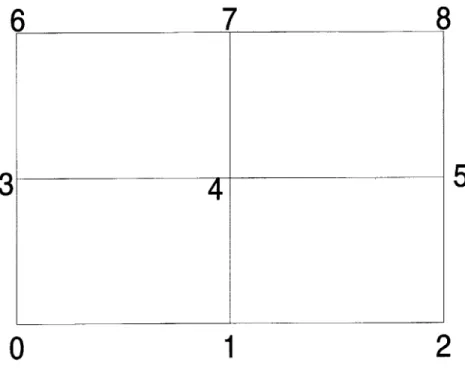
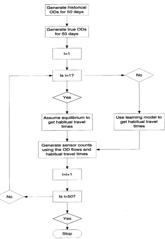
Grid network . . . . Flow chart for data generation . . . .

Sensor locations not capturing full information . . . .

Sensor locations capturing full information . . . .

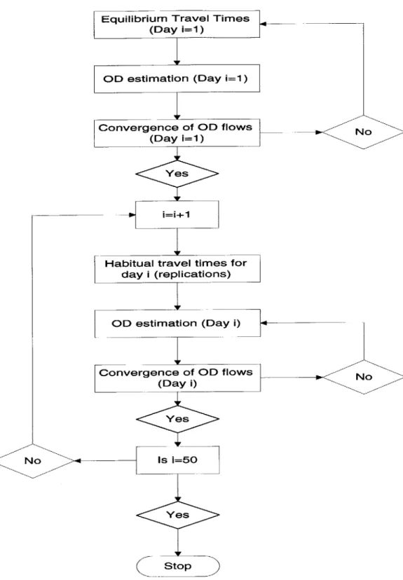
Sequential estimation of day-to-day OD flows . . . .

RMSE: True ODs vs Estimated ODs (All 50 days) . . RMSPE: True ODs vs Estimated ODs (All 50 days) RMSE: True ODs vs Estimated ODs (Last 10 days) RMSPE: True ODs vs Estimated ODs (Last 50 days)

M 27 network . . . .

4-12 Day-to-day variation of counts from 6:15AM to 7:30AM at 15min in-tervals . . . . 4-13 Day-to-day variation of counts from 7:45AM to 8:45AM at 15min in-tervals . . . . 4-14 Count comparison when OD flows are not assumed to vary . . . . 4-15 Count comparison when OD flows are assumed to vary . . . .

A-1 OD estimates for L-NF case (a) . . . . . . . . 2 1 . . . . 24 42 47 . . . . 53 . . . . 55 . . . . 57 . . . . 57 . . . . 60 . . . . 64 . . . . 64 . . . . 65 . . . . 65 . . . . 68 69 70 72 73 80 . . .

A-2 OD estimates for L-NF case (b) A-3 OD estimates for L-F case (a)

A-4 OD estimates for L-F case (b)

A-5 OD estimates for H-NF case (a) A-6 OD estimates for H-NF case (b) A-7 OD estimates for H-F case (a) A-8 OD estimates for H-F case (b)

B-1 Variation of OD flows from 1 -+ 3

B-2 Variation of OD flows from 1 -+ 5

B-3 Variation of OD flows from 2 - 5

B-4 Variation of OD flows from 4 -+ 5

. . . . 8 1 . . . . 8 2 . . . . 8 3 . . . . 8 4 . . . . 8 5 . . . . 8 6 . . . . 8 7 . . . . 9 0 . . . . 9 1 . . . . 9 2 . . . . 9 3

List of Tables

3.1 Possible assumptions on sources of variability in observed measurements . 37

4.1 Factors and their levels considered . . . . 58

4.2 RMSE: Observed counts Vs Simulated counts . . . . 62

4.3 RMSPE: Observed counts Vs Simulated counts . . . . 62

4.4 RMSE: True ODs Vs Estimated ODs (All 50 days) . . . . 62

4.5 RMSPE: True ODs Vs Estimated ODs (All 50 days) . . . . 63

4.6 RMSE: True ODs Vs Estimated ODs (Last 10 days) . . . . 63

4.7 RMSPE: True ODs Vs Estimated ODs (Last 10 days) . . . . 63

4.8 Estimated values of model parameters . . . . 71

4.9 Comparison of counts in both approaches . . . . 72

Chapter 1

Introduction

With the ever increasing travel needs of people, it is not surprising in the least to say that traffic congestion is among the foremost problems being faced by cities in developed as well as developing countries. As per the 2003 Urban Mobility Study re-port published by Texas Transre-portation Institute [29], the largest university-affiliated transportation research agency in the US, traffic congestion in 2001 resulted in the loss of 3.5 billion hours of productivity valued at $69.5 billion. A similar study by the

UK government estimates that 1.6 billion hours were lost by drivers and passengers

in 1996 due to congestion. The situation is not very different in the developing coun-tries, where the growth rate of fleet size is 10-30 per cent per year as against below 5

per cent in developed countries [16].

While congestion cannot be eliminated completely, measures can be adopted to alleviate the traffic conditions. Transportation agencies generally use three types of strategies to manage congestion:

" construction

" managing travel demand

" improving operations

Construction Traditionally, construction of more roads has been the strategy adopted

having to face a variety of physical, economic, social and environmental con-straints. Furthermore, it provides only temporary relief for congestion because it tends to encourage further development and therefore traffic growth. Most importantly, it is not possible to catch up with the growth rate in traffic. In-crease in route miles of highways in the US by about 1.5 per cent as against 76 per cent increase in vehicle miles between 1980 and 1999 illustrates this clearly.

Managing travel demand This strategy aims at altering driver behavior so that

vehicle trips during congested periods and at congested locations are reduced. Some of the programs which belong to this category are flexible work schedules that allow employees to travel off-peak, amenities to improve safety and effi-ciency of biking and walking, ridematching services for vanpools and carpools, community-based carsharing, employer-subsidized transit passes, guaranteed emergency rides home for transit users, incentives to decrease employer-paid parking and transit-oriented regional development.

Improving operations This method essentially tries to make use of the

transporta-tion system to the best extent possible through some strategies and thus tries to increase the efficiency and reliability of the system. Some of these strategies are: Advanced Traffic Management Systems (ATMS), Advanced Traveler In-formation Systems (ATIS), Incident Management Systems and Managed lanes (HOV lanes, truck-only facilities, congestion pricing, reversible and contra-flow roadways). These also involve altering the driver behavior.

1.1

Intelligent Transportation Systems

Intelligent Transportation Systems (ITS) is nothing but a composition of a number of technologies including information processing, communications, control and electron-ics applied to improve operations of the transportation systems. It was introduced as Intelligent Vehicle Highway Systems (IVHS) in late 80s with the multiple objectives of improving safety, reducing congestion, enhancing mobility, reducing environmental

impact, saving energy and increasing economic productivity. The five functional areas that have been identified for implementation of advanced technologies are Advanced

Traffic Management Systems, Advanced Traveler Information Systems, Advanced Ve-hicle Control Systems, Commercial VeVe-hicle Operations and Advanced Public Trans-portation Systems [22].

1.2

Microscopic simulation models

Traffic management strategies using the aforementioned advanced technologies may be counter productive if not implemented correctly, as shown by some studies (Gartner et al. [21]). Additionally, often there would be many feasible alternatives that could be adopted to deal with congestion problem in a particular region. While coming up with the feasible alternatives is not very difficult, identifying the best alternative is a hard task. Therefore, evaluation of the alternatives is a critical component in the development of an efficient strategy. These evaluations can be performed with the help of either field tests or simulation models.

Field tests involve implementing all the identified alternatives and choosing the

best among them based on certain measures of performance. Disadvantages of these tests are that they are time consuming and are not economical. Further, the test results are affected by uncontrollable parameters. In the case of ATIS, if some of the implemented alternatives do not improve the situation, it might affect the travelers' compliance with guidance provided in the future.

Simulation models , on the other hand, provide a very economical way of analyzing

the alternatives. Obviously, credibility of the results obtained from such a model is dependent on its ability to replicate reality to the best extent possible. Some of the microscopic simulation models which have been developed are MITSIMLab

[8], PARAMICS [30], FLEXSYT-II [34], etc. More detailed information on various

1.3

Calibration of microscopic simulation models

All the microscopic simulation models require demand for the use of the road network,

in the form of Origin - Destination (OD) flow matrix, as a necessary input. Each

element in this matrix represents the number of trips from a specific origin to a specific destination. Another important set of inputs to the microscopic simulation models is the underlying behavior model parameters. However, many of these parameters are network dependent. Therefore, before applying the simulation model to a network, it should be calibrated and validated for that particular network. In addition to OD flows and model parameters, habitual travel times form another set of inputs to the

simulation model.

Calibration is the process of determining the OD flow matrix and the behavior

model parameters so that the simulator reflects the local traffic conditions being modeled. Validation is the process of determining the extent to which the calibrated model can accurately replicate traffic behavior.

1.3.1

OD

flows

In practice, OD flows are not available and so need to be estimated. Cascetta [10], classifies the various methods of estimation of OD flows into three groups.

" direct sample estimation

" model estimation

" estimation from traffic flows

Direct sample estimation methods involve conducting surveys, such as home or

destination interviews, roadside interviews, flagging techniques or combination of them and estimating the OD flow matrix with these survey results using sampling theory classical estimators. Model estimation methods, which are commonly used, estimate OD flow matrix by applying a system of models that give the number of journeys made as a function of several socio-economic variables. The third method

of estimating OD flow matrix from traffic flows is a more recent one. This problem

can be understood as the opposite of traffic assignment problem. This method has received a lot of attention owing to its cost effectiveness as compared to conducting surveys. Furthermore, these flows can be measured repeatedly so that evolution of the phenomenon can be followed.

Since this thesis deals with only the third method of estimation, it should be understood that henceforth the terms "OD estimation" and "Estimating OD flows from traffic flows" are used interchangeably.

1.3.2

Behavior model parameters

Behavior model parameters are the other set of inputs to a microscopic simulation model which need to be estimated. These parameters can be classified into two groups, namely, travel behavior and driving behavior parameters. Travel behavior relates to decisions taken by drivers at a higher level and is represented by a route choice model. Driving behavior models, on the other hand, represent the decisions taken by drivers at micro level as a reaction to other vehicles in the vicinity. Some of these models include lane-changing, car-following and intersection models. These models will be discussed briefly in chapter 4.

1.3.3

Habitual travel times

Habitual travel times represent the drivers' perceptions of travel times based on which they make the route choice decisions. They cannot be measured since they represent perceptions of the travelers. Usually, the network is assumed to be in equilibrium (i.e, the travel times which the drivers expect on the network are consistent with what they experience) in order to estimate these habitual travel times.

1.4

Calibration methodology

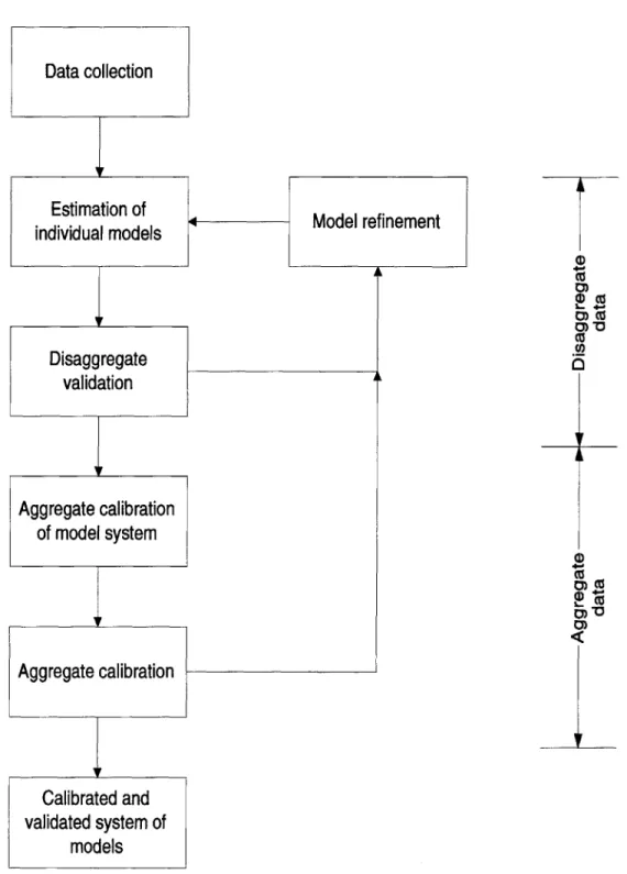
The typical methodology followed for calibration of microscopic simulation models is based on the framework shown in Figure 1-1 (which is reproduced from Ben-Akiva et al [7]). According to this framework, calibration involves two steps. In the first step, individual models (driving behavior and travel behavior models) that make up the simulation model are statistically estimated using disaggregate data such as trajectory data. In the second step, aggregate data (flows, speeds etc) is used to fine tune these parameters and estimate the OD flows. Using aggregate data to fine tune parameters helps in capturing the inter-dependencies among the parameters. But in most cases disaggregate data, being very expensive to collect, is not available. Therefore, calibration of the model parameters also has to be done using aggregate data only.

This problem of (i) estimating the OD flows and (ii) calibrating the model param-eters using aggregate data is called aggregate calibration .

1.5

Thesis focus

In this thesis, a general formulation for calibration of microscopic simulation models in the presence of multiple days of aggregate data will be proposed. Further, various assumptions one could make to simplify the formulation will be presented. Finally, the application of this general formulation is demonstrated through some case studies with focus being more on OD estimation.

1.6

Thesis outline

This thesis is organized as follows. In chapter 2, a brief review of the different methods

adopted for both components of aggregate calibration -OD estimation and parameter

calibration - is presented. In chapter 3, aggregate calibration in the presence of

mul-tiple days of data is formulated as an optimization problem and various assumptions that could be made to be able to solve the problem are outlined. In chapter 4

MIT-Data collection

Estimation of

individual models Model refinement

CO O)CU O)V CO a,) 0)"

Figure 1-1: Calibration Framework

Disaggregate validation Aggregate calibration of model system Aggregate calibration Calibrated and validated system of models i k

SIMLab, the microscopic simulation model which has been used in the following study is introduced. Case studies demonstrating the feasibility of the proposed calibration methodology are also discussed. Finally, conclusions drawn from the implementation of this methodolody and directions for future research are presented in chapter 5.

Chapter 2

Literature Review

The problem of aggregate calibration, which involves OD estimation and parameter calibration, has received a great deal of attention during the past few years. This chapter reviews literature pertaining to OD estimation, parameter calibration and obtaining user equilibrium travel times. Since the thesis focuses more on OD estima-tion, the other two are not discussed in detail.

2.1

OD

estimation

In this section, various methods proposed for the estimation of OD flows from aggre-gate measurements (traffic counts) are reviewed. Most of the following review can be found in the book by Cascetta [11].

This problem of estimating OD flows by combining traffic counts with other avail-able information is also referred to as origin-destination count based estimation

(OD-CBE) problem. Typically information on OD flows contained in traffic counts is not

sufficient enough to identify a unique set of OD flows. This is because of the relatively high number of OD pairs as compared to the number of links on which sensor mea-surements are available. Therefore additional information, giving apriori knowledge of the OD flows, is needed to estimate a unique set of OD flows. An overview of the inputs and outputs of the OD estimation problem can be seen in figure 2-1. In literature, apriori information on OD flows is also referred to as direct measurements

Sensor

Apriori

Counts

information

-

OD estimation

₄

OD

flow

estimates

Figure 2-1: Overview of OD estimation inputs and outputs

while traffic counts are referred to as indirect measurements (since they represent a function of the true OD flows intended to be estimated).

OD matrices estimated can be either static or dynamic in nature, depending on

the purpose of the study. A static OD matrix represents the average travel demand in a day, while a Dynamic OD matrix captures the temporal variation of travel demand within a day.

2.1.1

Static OD estimation

Methods which have been used for static OD estimation are entropy maximization or information minimization (Van Zuylen and L.G. Willumsen [37]), maximum like-lihood estimation (Spiess [33]), generalized least squares (Cascetta [10]; McNeil et al. [28]; Bell [6]) and bayesian estimation (Maher [27]). Some of these are described briefly below.

Maximum likelihood estimators are obtained by maximizing the probability of

ob-serving the apriori information and the sensor measurements. Making the reasonable assumption that these two probabilities are independent, the maximum likelihood

estimator can be expressed as:

XML = arg max[lnL(xH/x) + lnL(y/x)]

XES (2.1)

where:

x is the travel demand vector to be estimated

xH is the apriori information on the travel demand, which could be

obtained from sampling surveys or earlier planning studies

y is the vector of observed traffic counts

lnL(xH/x) is the log-likelihood function of the apriori information on travel de-mand, i.e. the logarithm of the probability of observing the apriori

travel demand xH is x is the true travel demand

lnL(y/x) is the log-likelihood function of the traffic counts, i.e. the logarithm of the probability of observing the traffic counts y if x is the true travel demand

S is the feasibility set of the true travel demand, usually coincident

with the non-negative orthant, i.e. S = x : x > 0

The log-likelihood functions in the equation (2.1) can be formulated after

assump-tions are made on the probability distribuassump-tions of xH and y, conditional on x.

Generalized Least Squares is another estimator based of classical statistics. This

can be derived from the system of linear stochastic equations (2.2) and (2.3) men-tioned below.

y = Ax

+

XH

(2.2)

(2.3)

with the following additional assumptions

E(c) = 0, Var(e) = V

A is called Assignment matrix . This matrix is nothing but a mapping between the traffic counts and the OD flows. The GLS estimator of the travel demand, which is the best linear unbiased estimator, can be expressed as:

XGLS= argmin[(y - Ax)'V- (y - Ax) + (xH - x)'W-(xH - x)] (2.4) xES

Bayesian estimation methods combine sampling information with prior or

sub-jective information. In this particular problem of OD estimation, bayesian estimation involves updating the OD flows obtained apriori with the additional information from traffic counts. The estimator is obtained from the a posteriori distribution h(x/y, xH), of OD flows conditioned on the apriori information and traffic counts. According to Bayesian theory, this posterior probability is proportional to the product of the apri-ori probability distribution of OD flows g(x/xH) and the probability of observing the traffic counts conditional upon the unknown OD flows L(y/x). Mathematically, this is expressed as:

h(x/y, xH) x L(y/x)g(x/xH) (2.5)

Bayesian estimator of OD flows can be obtained by maximizing the a posteriori probability in equation (2.5) or its natural logarithm (since natural logarithm is a monotonous function).

XB = arg max[lng(x/xH) + lnL(y/x)] (2.6) xES

As in the case of Maximum Likelihood estimator, the specification of the Bayesian estimator depends on the assumptions made for the probability distributions g(x/xH) and L(y/x).

Cascetta and Nguyen [13] examined Maximum Likelihood and Generalized Least Squares estimators and compared them to Bayesian estimator. They also discuss the computational issues for each of the approaches.

2.1.2

Dynamic OD estimation

The disadvantage of a static OD is that they only represent average traffic conditions in a day. They do not capture the temporal variation within a day and hence are not very useful for applications at operational level. Owing to this reason, several researchers have investigated the problem of dynamic OD estimation.

Various methods of dynamic OD estimation have been proposed, some of which (Cremer and Keller [17]; Bell [6]; Chang and Tao [15]) are are restricted to intersec-tions, junctions or small segments of network corridors and hence not applicable to general networks. A brief review of these estimation methods and the contexts in which they are applicable can be found in Ashok [3]. On the other hand,

General-ized Least Squares approach and Kalman Filter approach can be applied to general

networks. Refer to Ashok [3] and Balakrishna [4] for more information on these two approaches.

Generalized least squares

Cascetta et al. [12] have extended the generalized least squares estimation approach

to the dynamic case as well. Let the total period under consideration (H) be divided into T intervals, which can be assumed to be of equal length without loss of generality.

Let n, and nOD be the number of sensors in the network and the number of OD pairs

respectively. Let Xh be the column vector (nOD x 1) of travel demand of all the OD

pairs during interval h; and x' be the column vector of apriori OD flows for interval

h. Similarly, let Yh the corresponding column vector (n, x 1) of traffic counts measured

in interval h by all sensors.

The linear stochastic equations in the dynamic case are similar to equations (2.2) and (2.3):

h

Yh A AhXP +Vh (2.7)

p=h-p'

Xh =xh+Uh (2.8)

journey, A' is the assignment matrix which relates the flows departing in interval

p to counts observed in interval h. Vh and Uh are vectors of random errors. Let

variance-covariance matrices of Vh and Uh be Vh and Wh respectively.

They proposed two estimation procedures - simultaneous estimation and

sequen-tial estimation. In the simultaneous estimation approach, OD flows for all the inter-vals are estimated in a single step using the traffic counts for all the interinter-vals. The

OD flow estimates are given by:

T

(P 1, 2,... ,T) = argmin E[(xh - xh)'Whj(xh - Xh

h=1

T h h

+ [(Yh - E Apxp)'Vh-1(yh - APxP)] (2.9)

h=1 p=h-p' p=h-p'

with non-negativity constraints, xi > 0, Vi 1, 2, ... , T.

On the other hand, in sequential estimation approach the OD flows for all the intervals are estimated one at a time. When estimating the OD flows for interval h, the OD flow estimates of past intervals are kept constant. Hence the counts of period

h are linear functions of the unknown demand of the same period only. The OD flow

estimates of an interval h are given by:

Jh = argmin[(xh - x')'WWT(xh - x

h-1 h-1

+[(yh- E ApiP - A h )hVj 1(yh- A -h, ~ A xh) (2.10)

p=h-p' p=h-p'

Simultaneous estimation gives more consistent results, but it involves solving a very complex optimization problem. Hence, in practical situations where computational considerations are of prime importance, sequential estimation approach can be em-ployed.

Kalman filtering

This approach casts OD estimation problem as a state-space model. A state-space

-measurement equation and transition equation. The -measurement equation (2.11) relates the unknown state of the system to the observable data, and the transition equation (2.12) describes the evolution of system over time.

yh = Ahxh + Vh (2.11)

hh+1 hXh + Wh (2.12)

In the context of OD estimation, the set of equations (2.7) and (2.8) together form the measurement equations (2.15). Equation (2.12) represents the transition equation.

h-1

Yh _{ya E} A A _{,P = AJz +X} =Ah vh(.3 _(2.13)

p=h-p'

XH =Xh+Uh (2.14)

Expressing both equations (2.13) and (2.14) using matrix algebra, we have

_

1X.~

1[h

[Yh Ez=hp hP]

[uh

Xh +

Xh InROD U

or

yh = Ahx, + Ch (2.15)

The kalman filter algorithm, which is recursive in nature, is described here. Let

njk and Anik denote the OD flow estimates and their variance covariance matrix of

period n based on observations upto period k respectively. Let wh be white noise with zero mean and variance Qh. Similarly, let the variance of Ch be Ch. Assuming

that the initial system state is known (iolo = po and Ao0 o = Ao), the steps in the

algorithm are:

transi-tion equatransi-tion. Equatransi-tions (2.16) and (2.17) are referred to as predictor equatransi-tions.

Xhlh-1 = Oh-1Xh-1jh-1 (2.16)

AhIh-1 = Oh-1Ah-1Jh-1Oh-1 + Qh-1 (2.17)

2. Compute the kalman gain matrix

Kh = Ahh1A' (AhAhh_1A' + Ch)-1 (2.18)

3. Generate the filtered estimate and the corresponding variance covariance matrix

using the measurement equation. Equations (2.19) and (2.20) are referred to as corrector equations.

Xhlh = ihlh-1 + Kh(yh - Ah'hlah1) (2.19)

Ahh = Ahlh_1 - KhAhAhhl-1 (2.20)

4. Increment h and go back to step 1.

Many variations of this basic kalman filter algorithm have also been proposed. This method finds special use in on-line applications where prediction of traffic conditions is needed.

2.2

Parameter calibration

The problem of parameter calibration involves identifying the correct set of param-eters to be used in the underlying behavior models which reproduce the observed sensor measurements. This is very complex because of the absence of a clear analyt-ical formulation for the objective function in terms of the variables to be estimated. Various methods for calibrating parameters that have been used are:

- linear search (Balakrishna [4])

- simplex-based approach (Kim and Rilett [24])

- steepest descent (Kurian [25])

- box algorithm (Darda [19], Toledo et al. [36])

- genetic algorithms (Abdulhai et al. [1], Lee et al. [26])

2.3

Equilibrium travel times

Equilibrium implies that the habitual travel times based on which the drivers make their route choice decisions are consistent with what they experience on the network. These travel times are a property of the true behavioral models. Since the simulation model is used to approximate reality, the same can be used to obtain these equilibrium travel times. If S( is used to denote the simulation model and TT to denote the equilibrium travel times, then TT is a solution to the following equation (2.21).

TT = S(TT) (2.21)

This is nothing but a fixed point problem. Various iterative schemes have been proposed to solve this problem. Refer to Cascetta et al [14], Bottom [9] for a review. The studies mentioned in the above sections concentrate on one of the problems only and not the calibration of all the input parameters jointly. Other studies like Darda et al [19] and Jha et al [23] have captured the interactions between the param-eters by calibrating them jointly. Though aggregate calibration is the focus of this thesis, it has to be referred that validation of the calibrated simulation models is also an important task. In their paper, Toledo et al [36] have described various statistical measures that can be used to perform validation, but they do not take into account the correlations among the measurements. Barcelo et al [5] proposed a method for calibration and validation to account for these correlations between the sensor mea-surements. This method was implemented to calibrate the parameters of route choice

model. But it is not easily scalable because it involves manually looking for good set of parameters. Additionally, some useful guidelines for developing simulation models have been presented in the paper.

2.4

Summary and Motivation

When data is available for many days, it is not surprising if the sensor data is not the same for all the days. While this variation could be partly because of pure noise, there are few other possible reasons for this. Observed data could vary from day-to-day because of changes in

- model parameters

- travel demand (OD flows)

- habitual travel times

- network conditions (which includes weather conditions)

But the earlier approaches assume that the variation in observed data is purely be-cause of randomness and estimate a single OD matrix for all the days. So we might be losing wealth of information that is hidden in the data. Additionally, since the earlier approaches estimate an average OD matrix for the entire duration under study, they are suitable only for planning purposes and not for operational purposes or re-liability studies (where information on distribution of OD flows over days is needed). Hence, the objective in this thesis is to incorporate the variation of the inputs from day-to-day in the calibration methodology.

Chapter 3

Problem formulation

In this chapter, an optimization based general formulation has been proposed for the problem of aggregate calibration in the presence of multiple days of data. The equivalent formulation under the generalized least squares approach has also been presented.

3.1

A general formulation

Before proceeding to the formulation, some of the important variables involved in this problem and the notation used to denote them are mentioned. These variables are:

" Observed aggregate measurements

" Simulated aggregate measurements

* Network conditions

* Travel demand (OD flows)

" Behavior model parameters

" Habitual travel times

3.1.1

Notation

N number of days for which data is available

K 1,2, ... . N

mfobs observed measurements on day i

MiIM simulated measurements on day i and replication w. Simulation

models are stochastic in nature. Hence the simulated measurements are random variables.

Mistm mean simulated measurements on day i

Mim = E[Mim]

Gi network conditions on day i

Gy)j network conditions on days 1, 2, ... , i

Gy)] = {Gi, G2, ... , Gi}

ODj OD flows on day i

OD? apriori information on OD flows on day i

ODg)j OD flows on days 1, 2,...,i OD[] = {OD1, OD2, ... , ODi}

behavior model parameters for day i

,3j apriori information on behavior model parameters for day i

3[i] behavior model parameters on days 1, 2,. .. , i

,3 = {1,02, ... , 1i}

Tjihab habitual travel times for day i

TTjhab habitual travel times for days 1, 2, ... , i

TThab = {TThab, TThab hab

[i] 1TT T2 b,... ITTb

TTiewxp experienced travel times for day i and replication w. Since simula-tion model is stochastic, the simulated experienced travel times are random variables.

TTe"P mean experienced travel times for day i

T T"x = E[TTfewp ]

T rj'p mean experienced travel times for days 1, 2,... , i TijP = {TTXP, TT2"X, ... , TTie'P}

SM function which relates the inputs of a simulation model to the

sim-ulated measurements

STT function which relates the inputs of a simulation model to the

sim-ulated experienced travel times

3.1.2

Model equations

The equations which relate the measurements (both direct and indirect) of OD flows and model parameters to their true values form the basis of the optimization based methodology.

Mfbs = Mis8m + E, Vi EA (3.1)

OD = ODi + y , Vi E J (3.2)

/o = / + 6i, Vi G A (3.3)

Equation (3.1) represents indirect measurements while equations (3.2) and (3.3) rep-resent the direct measurements of OD flows and model parameters. Ei, 'yi and 6i represent the errors made in these measurements for day i.

3.1.3

Objective function

Let fi(Mobs, Mim) represent the measure of deviation of the observed sensor

mea-surements from the mean sensor meamea-surements produced by the simulation model for

day i. Similarly, let f2(ODi, OD9) and f3(i, Oi3) represent the measures of deviations

of the estimated OD flows from the apriori OD flows on day i and estimated model parameters from the apriori model parameters on day i respectively. The sum of all the three deviations for all days can serve as the objective function to be minimized:

N

f1(Mobs, Mfis) + f2(ODi, ODO) + f3(0i,

ly)

Without the second and third terms, the objective function will typically have multi-ple minima. So, with the inclusion of these two terms also in the objective function,

we aim to match the observed sensor measurements and at the same time we try not to deviate much from the apriori information we have on the OD flows and model parameters.

3.1.4

Constraints

This optimization problem would have two sets of constraints -expressions for

simula-tion outputs and the feasibility condisimula-tions for the OD flows and model parameters to be estimated. Equation (3.4) defines the simulated measurements used in the objec-tive function as a function of model parameters, OD flows, habitual travel times and network characteristics. w is random seed which is used to represent the stochastic nature of the simulator. Equation (3.6) describes how drivers update their habitual travel times day-to-day and is usually referred to as learning model in literature. The equation means that the habitual travel times on a day are a function of the habitual travel times and mean experienced travel times of all the previous days. Equation

(3.5) defines the experienced travel times used in equation (3.6) as a function of the

inputs to the simulation model and random seed.

Mis' = SM(3i, ODi, TT GabG, w) (3.4)

= STT (0, OD,TT habG ,W) (3.5)

T Thab = g(TT jabT Trej ) (3.6)

The other set of conditions are that the OD flows estimated should be non-negative and the estimated model parameters lie within a feasible region.

3.1.5

Complete formulation

The complete formulation would therefore be:

N

[

min E

f,

s.t. M"'7 = SM(/,OD, TIabGh )

T irT7x =ST T

(oi,

TThab = g(TT TTpy)x,

Only OD flows and model parameters are considered to be the decision variables because the the habitual travel times are dependent on the inputs for the previous days and the network conditions on all the days under consideration are assumed to be known.

3.1.6 Possible assumptions

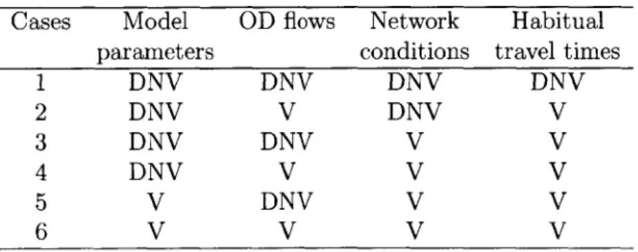
As noted earlier, the observed measurements will vary from day-to-day and the vari-ability in these measurements could be because of stochasticity or changes in OD flows, model parameters, network conditions and habitual travel times. The optimiza-tion problem presented in secoptimiza-tion (3.1.5) is very difficult to solve. Hence, depending on the purpose of the study, assumptions need to be made on the sources of variability in observed measurements. Since there are four possible sources of variability

(ex-cluding randomness which is always supposed to exist), there will be 24 = 16 possible

assumptions one can make.

But it is not logical to assume that the habitual travel times vary (do not vary)

when none of the others vary (at least one of the others varies) . It is also not logical

Cases Model OD flows Network Habitual

parameters conditions travel times

1 DNV DNV DNV DNV 2 DNV V DNV V 3 DNV DNV V V 4 DNV V V V 5 V DNV V V 6 V V V V

to assume that model parameters vary while the network conditions do not vary. Because of these conditions, the number of possible cases comes down to 6. These cases are mentioned in the table (3.1). In the table 'DNV' stands for do not vary and 'V' stands for vary .

Even for each of these cases, additional assumptions need to be made to be able to solve the problem. Cases 1 and 6 are the two alternative assumptions one can make and cases 2 to 5 are special restricted cases of these two cases. Formulations for cases 1 and 6 (referred to as stationary state and non-stationary state respectively) are presented.

3.1.7

Stationary state formulation

As per the assumptions, observed measurements vary from day-to-day purely because of randomness and none of the input parameters vary. Since habitual travel times are assumed not to vary, an additional assumption that the network is in equilibrium needs to be made to keep the problem solvable. As per the definition of equilibrium, the experienced travel times of drivers are consistent with the travel times they ex-pect (i.e., habitual travel times). The final formulation is shown in equation (3.8).

Note that the subscripts for /, OD, TThab, Ms'm and G have been avoided indicating that they do not vary. But since observed measurements vary (because of

random-ness), subscripts for Mobs have been used. This particular formulation for aggregate

calibration has been used by Darda [19].

N

Min :e f(Mi4bs, Msim) + f₂(OD, OD0) +

f3(0, 00)]

OD;>OES 1=

s.t. Mm = SM(03,OD,TThabG)

TTe"P = STT(, OD, TThab, G)

3.1.8

Non-stationary state formulation

The non-stationary state formulation, where we assume that all inputs vary, is nothing but the general formulation in section (3.1.5). It can reasonably be assumed that the

network conditions are finite in number and that the model parameters on any two days are different if and only if the network conditions on both the days are different.

Let ci represent the network conditions on day i. Also, let ci belong to a finite

set K. Since model parameters for a day have been assumed to be dependent only on the network conditions of that day, fi can be replaced by 0c,. In addition, it can also be assumed that the travelers update their habitual travel times based on their experiences on earlier days with similar network condition. The underlying premise is that the travelers are aware of the network conditions before they embark on their journey. With these set of assumptions, the formulation would be:

min

3])

ODi;>O,#ciESc f1(ioiOl

s.t. i = SM(/Ci, ODi, T Tab, G.) T T|' = STT(3c., ODi, TTihab, Gi)

TTnab = g(TrThabT TpxP)

where i* stands for set of days defined as i* =

{j/(j < i),

TTieP are the habitual travel times and experienced travel times respectively of all

days which belong to the set i*.

3.2

Generalized least squares formulation

Let Yih represent the sensor measurements on day i and interval h. Let yi be the

measurements in all intervals on day i and y be the vector of all the measurments. Let T be the number of intervals and N be the number of days. Then,

Similarly, let the OD flows to be estimated and their apriori information be arranged in two column vectors OD and ODO respectively. The model equations corresponding to those in section (3.1.2) would be (3.10) and (3.11). Note that apriori estimates of model parameters are typically not available and hence have not been incorporated in the model equations.

y obs -ysim +6 (3.10)

ODO = OD + (3.11)

Let 6 and -y have means of zero. Let variance covariance matrices of 6 and -y be

V and W respectively. Representing them in a single matrix, the variance covariance

matrix would be

V 0 0 W

Here, e and -y are assumed to be uncorrelated. Since the direct and indirect measure-ments are obtained from two different sources, this assumption is reasonable.

3.2.1

Objective function

As per Gauss-Markov theorem in Econometrics, Generalized least squares is the best linear unbiased estimator. The objective function to be minimized to obtain the GLS estimator of the unknown OD flows and model parameters is given by

Yobs _ ysim _{Y obs _ sim}

(.2

si 1 -y

1(3.12)

ODO-OD J LODO-OD

which upon simplification becomes

(y obs - ysim )'v-1(yobs - ysim) + (ODO - OD)'W-1(ODO - OD) (3.13)

measurements replaced by yfim and yobs respectively.

3.3

Solution approach

The GLS formulation presented is difficult to solve as it is. This is because there are

two sets of variables to estimated - OD flows and model parameters - which are very

different in their characteristics.

" OD flows are typically very large in number compared to model parameters.

" Objective function can be expressed analytically as a function of OD flows, but

not model parameters.

" Computational cost is very high for estimating model parameters as against

estimating OD flows because many efficient methods for OD estimation have been proposed over the years.

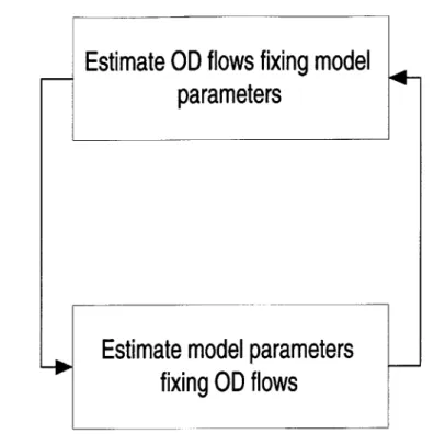
Hence, it would be efficient if these two sets of variables are separated and estimated iteratively as shown in figure (3-1).

The objective function to be minimized in these two sub-problems of OD estima-tion and parameter calibraestima-tion is (3.13). Note that for the sub-problem of parameter calibration, OD flows are held constant. Therefore removing the constant term from the equation (3.13) will not affect the estimates. The alternative objective function for parameter calibration would therefore be:

(yobs - ysim) v-(Yobs - ysim)

3.4

Estimating variance-covariance matrices

The variance covariance matrices V and W are not available. They need to be

estimated directly from the measurement errors c and -y. Let Eih and 'ih be the

measurement errors on day i and interval h. Since both within-day and day-to-day dynamics are being considered, we do not have multiple observations for measurement

Estimate OD flows fixing model

parameters

Estimate model parameters

fixing OD flows

Figure 3-1: Iterative method of optimization

errors to compute the variances and covariances from their definitions. Therefore additional assumptions need to be made to estimate these matrices.

The variance covariance matrices can be expressed as a function of a set of pa-rameters, which can then be estimated using the measurement errors. Alternatively,

weak stationarity can be assumed. Any times series X1, X2, ... , XT is said to be weakly

stationary if

E[xt] = [L, Vt

E[(xm - /)(Xn - A)] = E[(Xt+m - p)(Xt+n - [)], Vt

Essentially, it means that all the variables have the same mean and the covariance between any two of them is dependent only on the time lag between them.

Simi-larly, any two time series X1, x2, ... X, N and Y1, Y2, ... , YN are said to be jointly weak

E[xt] = p, Vt

E[yt] = v, Vt

E[(xm - p)(yn - v)] = E[(xt+m - P)(Yt+n - i)], Vt

Let 6

ih be the measurement error by a particular sensor on day i and interval h.

Then the series formed by these errors would be

611,612,... ,61H ... 6N1,6N2, .. ,6NH

where N is the number of days and H is the number of intervals per day. Assuming that the error terms within a day form a weakly stationary series, we have

1H-t

cov(6ih, 6i(t+h)) = N E th'(t+h') (3.14)

h'=1

Note that the variances of the error terms can be obtained by setting t = 0 in the

above equation. With joint weak stationarity assumptions, the covariance between the measurement error by a particular sensor on two different days can be estimated using the following equation

1H-t

COV(Zih,'(t+h)) = N h'6 i'(t+h') (3.15)

Nh'=1

Covariance between measurement errors of two different sensors can be computed sim-ilarly. Though only the calculation of V has been presented in equations (3.14) and

(3.15), W can be obtained similarly by replacing 6 with the corresponding

measure-ment error terms. Another method of estimating these variance covariance matrices could be assuming stationary processes such as AR(1). This is nothing but

Chapter 4

Case studies

In this chapter, results from two case studies which have been performed to demon-strate the feasibility of the proposed methodology of aggregate calibration are pre-sented. MITSIMLab (Microscopic Traffic Simulator Laboratory) has been chosen as the simulator to show the process of calibration. Before proceeding to the case studies, a brief overview of MITSIM has been presented.

4.1

Overview of MITSIM

MITSIM has been developed at MIT Intelligent Transportation Systems Lab by Yang

[38] to model traffic flow at the microscopic level. Significant contributions to the

de-velopment to MITSIM have also been made by Davol [20], Toledo [35]. It was devel-oped primarily to be able to evaluate the impacts of Advanced Traveler Information Systems (ATIS) and Advanced Traffic Management Systems (ATMS). MITSIMLab is a synthesis of a number of different models and has the following characteristics:

e represents a wide range of traffic management system designs

* models the response of drivers to real-time traffic information and controls * incorporates the dynamic interaction between the traffic management system

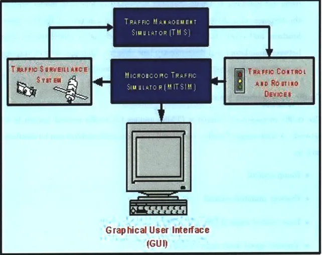
These are the main components of MITSIMLab:

" Traffic flow simulator (MITSIM) " Traffic management simulator (TMS) " Surveillance system

* Control and routing devices

The interaction between these components, which is shown in figure (4-1), is a critical element for a simulator. MITSIM is the traffic flow simulator and it models driver behavior and vehicular flow in the network at the microscopic level, while TMS is the traffic management simulator and it mimics the traffic control and routing functions chosen for evaluation. Traffic flow and route guidance affects the behavior of individual drivers, and hence, traffic flow characteristics as well. The changes in traffic flows are in turn measured by the surveillance system and consequently influence control and route guidance strategies. The simulator has a graphical user interface

(GUI) also that is used for both debugging purposes and visual demonstration of

traffic flow conditions through vehicle animation.

4.1.1 Components

Traffic flow simulator

MITSIM tries to replicate reality as well as possible. The traffic and network elements are represented in detail in order to capture the sensitivity of traffic flows to the control

and route strategies. The main elements in MITSIM are

" Network components: The road network along with the traffic controls and surveillance devices are represented at the microscopic level. The road network consists of nodes, links, segments (segments are parts of links with uniform characteristics) and lanes.

" Travel demand and Route choice: The simulator requires as input time-dependent

I

$

Grap hical User Interface (GUI)

Figure 4-1: Components of MITSIM and their interactions

a .... =75L -- l

as part of a scenario for evaluation. A probabilistic route choice model is used to capture drivers' route choice decisions.

o Driving behavior: The OD flows are translated into individual vehicles wishing to enter the network at a specific time. Behavior parameters (such as desired speed, aggressiveness, etc.) and vehicle characteristics are assigned to each vehicle/driver combination. The movement of these vehicles is then simulated using car-following and lane-changing models. Car-following model captures the response of a driver to conditions ahead as a function of relative speed, headway and other traffic measures. The lane-changing model distinguishes between mandatory and discretionary lane changes. Merging, drivers' response to traffic signals, speed limits, incidents and toll booths are also captured.

Traffic management simulator

The traffic management simulator (TMS) mimics the traffic control system in the network. A wide range of traffic control and route guidance systems can be simulated, such as:

" Ramp control

" Freeway mainline control

" Lane control signs (LCS)

" Variable speed limit signs (VSLS) " Portal signals at tunnel entrances (PS) " Intersection control

" Variable message signs (VMS) " In-vehicle route guidance

TMS has a generic structure that can represent different designs of such systems with logic at varying levels of sophistication (from pre-timed to responsive).

Surveillance system

The surveillance system measures the traffic conditions simulated by MITSIM and communicate them to the TMS. The following types of sensors can be simulated in MITSIMLab: Traffic sensors, Vehicle sensors, Point to point data sensors and Area wide sensors.

Control and routing devices

MITSIMLab supports a wide range of logics, including pre-timed signal controls, traffic adaptive controls, metering controls and control strategies in response to inci-dents. The vehicles respond to these signals or guidance according to some behavioral models.

4.1.2

Behavior models

In MITSIMLab vehicles move according to behavioral models, of which the most important ones are

* General acceleration

* Lane changing and gap acceptance

" Route choice models

General acceleration

A vehicle accelerates/decelerates in order to react vehicles ahead, perform a lane

changing or merging maneuver or to respond to events. Depending on the degree of interaction with the vehicle ahead, the subject can be in free-flowing, car-following or emergency regime. The degree of interaction is determined by the time headway between the two vehicles. The acceleration in the free-flowing regime is a function of the vehicle's desired speed, while in the car-following and emergency regimes, the acceleration is a function of traffic conditions and relative position and speed of the two interacting vehicles.

In the free-flowing regime, the vehicle accelerates if its current speed is different from the driver's desired speed. The acceleration applied by a driver in this regime is assumed to have the following functional form:

alf(t) = Aff [V*(t - Tn) - V(t - rn)] + 6 (t) (4.1)

where

czf(t) acceleration of driver n at time t

Aff parameter

V* (t) desired speed of the driver at time t

V1 (t) speed of subject vehicle at time t

Tn reaction time of driver n

ndt(t) error term

The car-following model is used for calculating a vehicle's acceleration or decel-eration rate in various cases such as: (i) Car-following relationship with the leading vehicle (ii) Competition with other vehicles if two or more lanes merge into a single downstream lane and (iii) Yielding to another vehicle shifting into the same lane It can be expressed mathematically as:

aof(t) = ,V(t - c_ k'[Vn ₁(t - rn) - Vn(t - rn)]' + cf (t) (4.2)

[Ax(t - r)

where

ae/(t) acceleration of driver n at time t

Ax(t) gap between vehicles at time t

k density of traffic in the vicinity of the vehicle

a, f, y, 6 parameters

In the emergency regime, the vehicle uses an appropriate deceleration rate to avoid collision. The deceleration rate depends on the state of the front and subject vehicles.