Buckling and damage resistance of transversely-loaded composite shells

BUCKLING AND DAMAGE RESISTANCE OF

TRANSVERSELY-LOADED COMPOSITE SHELLS

by

Brian L. Wardle

B. S., Aerospace Engineering

The Pennsylvania State University (1992) S. M., Aeronautics and Astronautics Massachusetts Institute of Technology (1995)

Submitted to the Department of Aeronautics and Astronautics in Partial Fulfillment of the Requirements for the Degree of

Doctor of Philosophy in Aeronautics and Astronautics

at the

Massachusetts Institute of Technology June 1998

@ 1998 Massachusetts Institute of Technology All rights reserved

Signature of Author ...

.r

f-...

Department of Aeronautics and Astronautics April 28, 1998 S... ... ... .. ... ...

Paul A. Lagace MacVicar Faculty Fellow, Prfesor of Aeronautics and Astronautics / I II Chairman. Thesis Committee

C ertifi ed by ... ... ...

Certified

John W. Hutchinson Gordon McKay Professor of Applied Mechanics, Harvard University Thesis Committee Certified by ... .... . ...

S. Mark Spearin Boeing Assistant Professor of A ronautics and Astronau I

I 1 rlh1his Committee

Accepted by Peraire

Associate Professor of Alrondutis and Astronautics Chairman, Department Graduate Committee

JULt O8

BUCKLING AND DAMAGE RESISTANCE OF

TRANSVERSELY-LOADED COMPOSITE SHELLS

by

Brian L. Wardle

Submitted to the Department of Aeronautics and Astronautics on April 28, 1998 in Painful Fulfillment of the

Requirements for the Degree of Doctor of Philosophy in Aeronautics and Astronautics

ABSTRACT

Experimental and numerical work was conducted to better understand composite shell response to transverse loadings which simulate damage-causing impact events. The quasi-static, centered, transverse loading response of laminated graphite/epoxy shells in a [±45n/0n]s layup having geometric characteristics of a commercial fuselage are studied. The singly-curved composite shell structures are hinged along the straight circumferential edges and either free or simply

supported along the curved axial edges. Key components of the shell response are response instabilities due to limit-point and/or bifurcation buckling.

Experimentally, deflection-controlled shell response is characterized via load-deflection data, deformation-shape evolutions, and the resulting damage state. Finite element models are used to study the kinematically nonlinear shell

response, including bifurcation, limit-points, and postbuckling. A novel technique is developed for evaluating bifurcation from nonlinear prebuckling states utilizing asymmetric spatial discretization to introduce numerical perturbations.

Advantages of the asymmetric meshing technique (AMT) over traditional

techniques include efficiency, robustness, ease of application, and solution of the actual (not modified) problems. The AMT is validated by comparison to traditional numerical analysis of a benchmark problem and verified by comparison to

experimental data. Applying the technique, bifurcation in a benchmark shell-buckling problem is correctly identified. Excellent agreement between the

numerical and experimental results are obtained for a number of composite shells although predictive capability decreases for stiffer (thicker) specimens which is attributed to compliance of the test fixture. Restraining the axial edge (simple support) has the effect of creating a more complex response which involves

unstable bifurcation, limit-point buckling, and dynamic collapse. Such shells were noted to bifurcate into asymmetric deformation modes but were undamaged during testing. Shells in this study which were damaged were not observed to bifurcate. Thus, a direct link between bifurcation and atypical damage could not be

established although the mechanism (bifurcation) was identified.

Recommendations for further work in these related areas are provided and include extensions of the AMT to other shell geometries and structural problems.

Thesis Supervisor: Paul A. Lagace

Acknowledgment

Many thanks to Paul for his efforts throughout this work. Thanks also to John Hutchinson and Mark Spearing for their comments and guidance. Thanks also to the other Profs. in TELAC and especially to Deb-ster and Ping for their help whenever needed. Thanks to John Kane for helping out in the lab. Of course, my UROPs did the real work: thanks to Doug MacIvor for helping get things started and Kim Murdoch who was there through experiments and STAGS til the bitter(?) end. Huge thanks and a shout out to Allen Waters down at Langley -Folks, that man knows his finite elements. Special thanks to my family and Gram for support over the years. Most of all, thanks to Cecelia for support and understanding -it meant a lot.

I used up all the good quotes in my Master's thesis. Speaking of which, the length of this thesis is 0.49 Wardles -I win.

-4-Foreword

This work was performed in the Technology Laboratory for Advanced Composites (TELAC) in the Department of Aeronautics and Astronautics at the Massachusetts Institute of Technology. This work was sponsored by NASA Langley Research Center under NASA Grant NAG-1-991.

Table of Contents

2.2.3 Finite Element Modeling ... ... 33

3 A P P R O A C H ... 39

3.1 General Overview ... 39

3.2 Numerical (Finite Element) Modeling ... .... 45

3.3 E xperim ents ... ... 48

4 FINITE ELEMENT MODELING ... ... 51

4.1 Modeling Overview ... 51

4.2 Asymmetric Meshing Technique for Bifurcation ... 54

4.3 Benchmark Shell Buckling Problem... 58

4.3.1 Comparison to Previous Work (Limit-point Buckling) ... 58

4.3.2 Bifurcation Buckling ... 61

4.3.3 Mesh Refinement and Convergence ... 73

4.4 Analysis of Previous Experimental Work ... 75

4.4.1 Description of Experiments... ... ... 77

4.4.2 Load-deflection and Mode-shape Comparisons ... 78

4.4.3 Modeling Assumptions and Experimental Realities... 93

5 EX PERIM EN TS ... ... 100

5.1 Manufacturing Procedures ... 100

5.1.1 Graphite/Epoxy Prepreg Layup ... .... 100

5.1.2 C uring ... ... 101

5.1.3 Final Specimen Preparation ... 107

5.2 Curvature and Thickness Mapping... .... 108

5.3 Test Fixture (Boundary Conditions) ... 113

5.4 Testing Procedures... ... 19

5.4.1 Specimen Set-up in Fixture...122

5.4.2 Quasi-static Testing and Mode-shape Measurement...124

5.5 Damage Evaluation... ... 128 6 RESU LTS ... 133 6.1 Experimental Observations ... 133 6.1.1 Loading Response... ... 133 6.1.2 Mode-shape Evolutions ... 143 6.1.3 Damage Development ... 166 6.2 Numerical Analysis ... 171 6.2.1 Loading Response ... 171 6.2.2 Mode-shape Evolutions ... 193 7 D ISCU SSIO N ... ... 207

7.1 Experimental and Numerical Comparisons ... 207

7.2 Boundary Conditions ... ... 228

7.2.1 Modeling Assumption at Circumferential (Hinged) Edge...228

7.2.2 Effect of Axial Edge Restraint... ... 233

7.3 Damage Resistance ... 245

7.4 Asymmetric Meshing Technique (AMT)...246

8 CONCLUSIONS AND RECOMMENDATIONS ... 249

8.1 C onclusions ... ... 249

8.2 Recommendations... 251

R eferences ... ... 254

Appendix A MANUFACTURING DATA...265

Appendix B NUMERICAL COMPARISON TO PREVIOUS ... 267 EXPERIMENTAL LOAD-DEFLECTION DATA

List of Figures

Illustration of typical shell instability [19]. Load-deflection curves showing limit-point and bifurcation buckling behavior (as in [43]).

Illustration of generic composite shell specimen.

Illustration of restrained shell with local coordinate system used to describe boundary condition at shell axial edge. Illustration of a 10 x 10 mesh and curvilinear shell

coordinate system. (The x and y (curvilinear) vectors are in the plane of the shell while z is everywhere perpendicular to the shell surface.)

Illustration of an asymmetrically meshed shell discretized into two shell units in the circumferential (y) direction. Configuration for benchmark shell problem.

Numerical analysis and previously reported results [61, 71] for load-deflection response of benchmark shell problem. Central spanwise deformation modes for benchmark

problem at different values of center deflection, we, using STAGS with a symmetric (10x10) mesh.

Load versus center and edge deflections for benchmark problem using STAGS with a symmetric (10x10) mesh. Load-deflection response for benchmark problem using STAGS with a symmetric (10x10) mesh incorporating scaled eigenmode imperfections into the initial geometry. Central spanwise plot of the linear bifurcation mode for benchmark shell problem.

Load-deflection response for benchmark problem using STAGS with a symmetric (10x10) mesh incorporating scaled eigenmode deformations (equivalence transform) near the bifurcation point.

Central spanwise deformation modes for benchmark problem at different values of center deflection, we, using STAGS with a symmetric (10x10) mesh and the equivalence transform method (2.0% thickness).

26 29 41 44 53 57 59 60 62 63 65 66 67 69

Figure 4.11 Figure 4.12 Figure 4.13 Figure 4.14 Figure 4.15 Figure 4.16 Figure 4.17 Figure 4.18 Figure 4.19 Figure 4.20 Figure 4.21 Figure 4.22 Figure 4.23

Load-deflection response for benchmark problem using STAGS with symmetric (10x10) and asymmetric (10x6 / 10x5) meshes.

Central spanwise deformation modes for benchmark problem at different values of center deflection, we, using

STAGS with an asymmetric (10x6 / 10x5) mesh. Load versus center and edge deflections for benchmark problem using STAGS with an asymmetric

(10x6 / 10x5) mesh.

Numerical analysis of load-deflection response for

benchmark shell problem using various asymmetric meshes. Load-deflection response for benchmark problem using

STAGS with asymmetric (20x12 / 20x9) and (20x12 / 20x5) meshes.

Central load-deflection results from numerical analyses and experiment [21] for the transverse buckling response of composite shell specimen R6S3T1.

Central load-deflection results from numerical analyses and experiment [21] for the transverse buckling response of composite shell specimen R12S3T1.

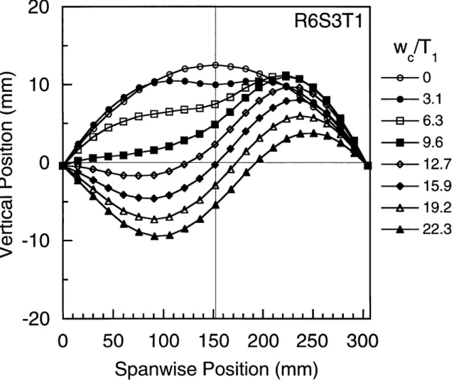
Numerical analysis results of central spanwise deformation modes for specimen R6S3T1 at different values of normalized center deflection.

Measured [21] central spanwise deformation modes for specimen R6S3T at different values of normalized center deflection.

Numerical analysis results of central spanwise deformation modes for specimen R12S3T1 at different values of normalized center deflection.

Measured [21] central spanwise deformation modes for specimen R12S3T1 at different values of normalized center deflection.

Numerical analysis results of central axial deformation modes for specimen R6S3T1 at different values of normalized center deflection.

Measured [21] central axial deformation modes for

specimen R6S3T1 at different values of normalized center deflection. 70 71 72 74 76 80 81 82 83 84 85 87 88

Figure 4.24 Figure 4.25 Figure 4.26 Figure 4.27 Figure 4.28 Figure 4.29 Figure 5.1 Figure 5.2 Figure 5.3 Figure Figure Figure Figure Figure Figure 5.4 5.5 5.6 5.7 5.8 5.9 Figure 5.10 Figure 5.11 Figure 5.12 Figure 5.13 Figure 5.14

Numerical analysis results of central axial deformation modes for specimen R12S3T at different values of normalized center deflection.

Measured [21] central axial deformation modes for specimen R12S3T1 at different values of normalized center deflection.

Numerical analysis results of central spanwise deformation modes for specimen R6S3T1 at different values of normalized

center deflection, we IT1, near the bifurcation point. Numerical analysis results of edge spanwise deformation modes for specimen R6S3T1 at different values of normalized

center deflection, wC / T1, near the bifurcation point. Load versus center and edge deflections from numerical analysis of specimen R12S3T1.

Central load-deflection results from numerical analyses and experiment [21] for the transverse buckling response of composite shell specimen R12S3T2.

Illustration of cylindrical mold. Cure assembly.

Nominal temperature, pressure, and vacuum profiles for cure cycle.

Locations used for mapping shell thickness.

Illustration of overhead view of curvature measuring setup. Measurements and associated locations used in radii and twist calculations.

Side-view illustration of original test fixture. Illustration of rod/cushion assembly.

Illustration of laser operation and grooved insert in the rod-cushion assembly.

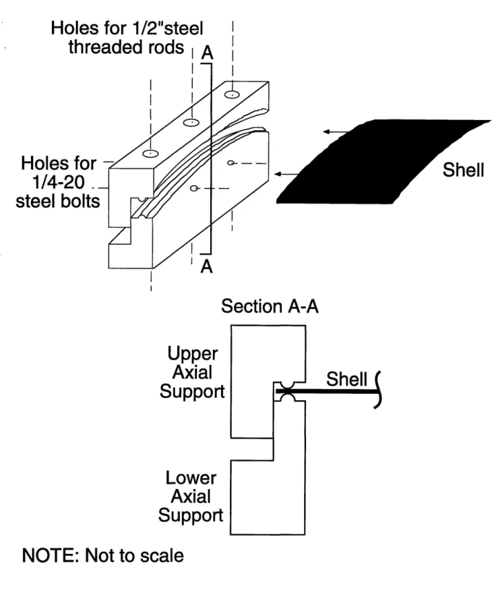
Illustration of test fixture modification used to restrain axial shell edges.

Three-view schematic (to scale) of lower support for axial shell edge. (Note: all dimensions in inches)

Three-view schematic (to scale) of upper support for axial shell edge. (Note: all dimensions in inches)

Illustration of test fixture and shell mounted in testing machine. Deflection-measurement assembly. 89 90 91 92 94 96 102 105 106 109 110 111 115 116 117 118 120 121 125 127

-10-Sample planar x-ray picture showing damaged region. Examples of visible damage in cross-sections of a T2 shell: (top) entire specimen thickness, and (bottom) magnified

view of lower right corner.

Figure 6.1 Figure 6.2 Figure 6.3 Figure 6.4 Figure 6.5 Figure 6.6 Figure 6.7 Figure 6.8 Figure 6.9 Figure 6.10 Figure 6.11 Figure 6.12 Figure 6.13 Figure 6.14 Figure 6.15 Figure 6.16 Figure 6.17 Experimental R12S3T1-1. Experimental R12S3T1-2. Experimental R12S3T2-1. Experimental R₁₂S₃T₂-2. Experimental R12S3T3-1. Experimental R12S3T3-2.

load-deflection response for specimen load-deflection response for specimen load-deflection response for specimen load-deflection response for specimen load-deflection response for specimen load-deflection response for specimen Experimental load-deflection responses for specimens

of different thicknesses.

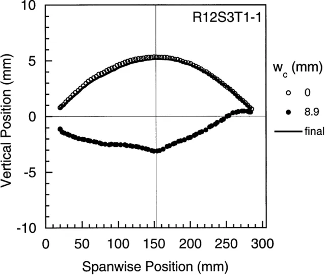
Measured central spanwise deformation modes for

specimen R12S3T1-1 at different values of center deflection. Measured left spanwise deformation modes for specimen R12S3T,-1 at different values of center deflection.

Measured right spanwise deformation modes for specimen R12S3T1-1 at different values of center deflection.

Measured central spanwise deformation modes for

specimen R12S3T1-2 at different values of center deflection. Measured left spanwise deformation modes for specimen R12S3T1-2 at different values of center deflection.

Measured right spanwise deformation modes for specimen R12S3T1-2 at different values of center deflection.

Measured central spanwise deformation modes for

specimen R12S3T2-1 at different values of center deflection. Measured left spanwise deformation modes for specimen R12S3T2-1 at different values of center deflection.

Measured right spanwise deformation modes for specimen R12S3T2-1 at different values of center deflection.

Measured central spanwise deformation modes for

specimen R12S3T3-1 at different values of center deflection.

135 136 139 140 141 142 144 146 147 148 149 150 151 153 154 155 156 Figure Figure 5.15 5.16 130 132

-11-Figure 6.18 Figure 6.19 Figure 6.20 Figure 6.21 Figure 6.22 Figure 6.23 Figure 6.24 Figure 6.25 Figure 6.26 Figure 6.27 Figure 6.28 Figure 6.29 Figure 6.30 Figure 6.31 Figure 6.32 Figure 6.33

Measured left spanwise deformation modes for specimen R12S3T3-1 at different values of center deflection.

Measured right spanwise deformation modes for specimen R12S3T3-1 at different values of center deflection.

Measured central spanwise deformation modes for

specimen R12S3T2-2 at different values of center deflection. Measured left spanwise deformation modes for specimen R12S3T2-2 at different values of center deflection.

Measured right spanwise deformation modes for specimen R12S3T2-2 at different values of center deflection.

Measured central spanwise deformation modes for

specimen R12S3T3-2 at different values of center deflection. Measured left spanwise deformation modes for specimen R12S3T3-2 at different values of center deflection.

Measured right spanwise deformation modes for specimen R12S3T3-2 at different values of center deflection.

X-ray photographs of specimen type R12S3T2 loaded to: (top) 1096 N (we = 16.0 mm), and (bottom) 1737 N

(wc = 19.1 mm).

X-ray photographs of specimen type R12S3T3 loaded to: (top) 1987 N (we = 15.0 mm), and (bottom) 2746 N

(we = 16.6 mm).

Load-deflection results from numerical analyses for specimen R12S3T1-1 using symmetric meshes. Load-deflection results from numerical analyses for specimen R12S3T1-1 using symmetric and asymmetric meshes.

Load-deflection results from numerical analyses for specimen R12S3T1-1 using various asymmetric meshes. Central spanwise bifurcation mode evaluated at 126 N for specimen R12S3T1-1 using a symmetric (20x20) mesh. Load-deflection results from numerical analyses of specimen R12S3T1-1 using a 20x20 symmetric mesh incorporating scaled eigenmode deformations (equivalence transform) near the bifurcation point.

Load-deflection results from numerical analyses of

specimen R12S3T1-1 using a 20x20 symmetric mesh and a 20x20 symmetric mesh with a 0.5% t imperfection based on the eigenmode in Figure 6.31.

157 158 159 160 161 162 163 164 168 169 173 175 177 179 180 182

-12-Figure 6.34 Figure 6.35 Figure 6.36 Figure 6.37 Figure 6.38 Figure 6.39 Figure 6.40 Figure 6.41 Figure 6.42 Figure 6.43 Figure 6.44 Figure 6.45 Figure 6.46

Load-deflection results from numerical analyses of

specimen R12S3T1-1 using a 20x20 symmetric mesh with 50% and 100% t imperfections based on the eigenmode in Figure 6.31.

Load-deflection results from numerical analyses for

specimens R12S3T-1 and R12S3T1-2 using an asymmetric (20x12 / 20x5) mesh.

Load-deflection results from numerical analyses for specimen R12S3T2-1 using symmetric and asymmetric meshes.

Load-deflection results from numerical analyses for specimens R12S3T2-1 and R12S3T2-2 using an asymmetric (20x12 / 20x7) mesh.

Load-deflection results from numerical analyses for specimen R12S3T3-1 using symmetric and asymmetric meshes.

Blow-up of Figure 6.38 in area of bifurcation: load-deflection results from numerical analyses for specimen R12S3T3-1

using symmetric and asymmetric meshes.

Load-deflection results from numerical analyses for specimens R12S3T3-1 and R12S3T3-2 using an asymmetric (20x12 / 20x7) mesh.

Load-deflection results from numerical analyses for specimens R12S3T1-1, R12S3T2-1, and R12S3T3-1 using asymmetric meshes.

Numerical analysis results of central spanwise

deformation modes for specimen R12S3T1-2 at different values of center deflection.

Numerical analysis results of left spanwise deformation modes for specimen R12S3T1-2 at different values of center deflection.

Numerical analysis results of right spanwise deformation modes for specimen R12S3T1-2 at different values of center deflection.

Numerical analysis results of central spanwise

deformation modes for specimen R1 2S3T2-2 at different values of center deflection.

Numerical analysis results of left spanwise

deformation modes for specimen R12S3T2-2 at different values of center deflection.

183 185 186 187 189 190 191 192 195 196 197 199 200

-13-Figure 6.47 Figure 6.48 Figure 6.49 Figure 6.50 Figure 7.1 Figure 7.2 Figure 7.3 Figure 7.4 Figure 7.5 Figure 7.6 Figure 7.7 Figure 7.8 Figure 7.9 Figure 7.10 Figure 7.11

Numerical analysis results of right spanwise deformation modes for specimen R12S3T2-2 at different values of center

deflection.

Numerical analysis results of central spanwise

deformation modes for specimen R12S3T3-2 at different

values of center deflection.

Numerical analysis results of left spanwise deformation modes for specimen R12S3T3-2 at different values of center

deflection.

Numerical analysis results of right spanwise deformation modes for specimen R12S3T3-2 at different values of center

deflection.

Illustration of deflection-controlled "snap" utilizing load-deflection results from numerical analyses for specimen

R12S3T1-1 (see Figure 6.29).

Numerical and experimental load-deflection results for specimen R12S3T-1.

Numerical and experimental load-deflection results for specimen R12S3T2-1.

Numerical and experimental load-deflection results for specimen R12S3T3-1.

Measured central spanwise deformation modes for

specimen R12S3T1-2 at different values of center deflection.

Numerical analysis results of central spanwise

deformation modes for specimen R12S3T1-2 at different

values of center deflection.

Measured left spanwise deformation modes for specimen

R12S3T1-2 at different values of center deflection.

Numerical analysis results of left spanwise deformation modes for specimen R12S3T1-2 at different values of center

deflection.

Measured right spanwise deformation modes for specimen

R12S3T1-2 at different values of center deflection.

Numerical analysis results of right spanwise deformation modes for specimen R12S3T1-2 at different values of center

deflection.

Measured central spanwise deformation modes for

specimen R12S3T2-2 at different values of center deflection.

201 203 204 205 209 210 211 212 216 217 218 219 220 221 223

-14-Figure 7.12 Figure 7.13 Figure 7.14 Figure 7.15 Figure 7.16 Figure 7.17 Figure 7.18 Figure 7.19 Figure 7.20 Figure 7.21 Figure 7.22 Figure 7.23 Figure 7.24 Figures B.1-B.18

Numerical analysis results of central spanwise

deformation modes for specimen R12S3T2-2 at different

values of center deflection.

Measured central spanwise deformation modes for

specimen R12S3T3-2 at different values of center deflection.

Numerical analysis results of central spanwise

deformation modes for specimen R12S3T3-2 at different

values of center deflection.

Numerical load-deflection results for specimen R1 2S3T1-1

utilizing different assumptions on the u-component of displacement at the circumferential boundary condition (hinged).

Numerical load-deflection results for specimen R12S3T2-1

utilizing different assumptions on the u-component of displacement at the circumferential boundary condition (hinged).

Numerical load-deflection results for specimen R12S3T3-1

utilizing different assumptions on the u-component of displacement at the circumferential boundary condition

(hinged).

Experimental load-deflection response of composite shell

R12S3T1 with axial edges restrained and free [21].

Numerical load-deflection results for composite shell

R12S3T1 with axial edges restrained and free.

Experimental load-deflection response of composite shell

R12S3T2 with axial edges restrained and free [21].

Numerical load-deflection results for composite shell

R₁₂S₃T₂ with axial edges restrained and free.

Experimental load-deflection response of composite shell

R12S3T3 with axial edges restrained and free [21].

Numerical load-deflection results for composite shell

R12S3T3 with axial edges restrained and free.

Experimental central spanwise deformation modes for specimen R12S3T1 at different values of center deflection

with axial edges free [21].

Loading response comparison from numerical analysis and experimental data [21] for composite shells.

224 225 226 230 231 232 235 236 238 239 240 241 243 269-286

-15-List of Tables

AS4/3501-6 Ply Data

Results of Thickness and Curvature Mapping Peak Load and Associated Center Deflection Radius and Thickness Data

Measured Values of Radius Used in Numerical Analysis Table 4.1 Table 5.1 Table 6.1 Table A. 1 Table B.1 77 113 167 266 268

Nomenclature

E Young's modulus

G shear modulus

n structural scaling parameter

R shell radius

Rn scaled shell radius

Rx rotation about x-direction

Ry rotation about y-direction

Rz rotation about z-direction S, scaled shell span

t shell thickness

Tn scaled shell thickness

u displacement component in x-direction

v displacement component in y-direction

w displacement component in z-direction

we w displacement at shell center x axial direction

X1 base for generic scaled structural variable

X, generic scaled structural variable

y curvilinear circumferential direction

z transverse direction /3 axial twist

7 spanwise twist

V Poisson's ratio

-17-CHAPTER 1

INTRODUCTION

Laminated composite materials continue to see increased use in structural applications. Performance advantages over traditional metallic structures abound: high specific stiffness and strength, mechanical tailoring capabilities, and excellent fatigue characteristics are some of the attributes that make structures built from laminated composites attractive to designers. This is especially true in the aerospace community where composites are seen to provide increased performance for both military and commercial structures.

In the aircraft industry, composites initially replaced secondary structures that were typically made from aluminum, e.g., [1, 2]. Damage considerations in the design of secondary structures are typically not critical. However, composites have seen increased application in design of primary aerospace structures where damage is a critical design issue. Primary composite structures in the V-22 Osprey, single-stage to orbit (SSTO) reusable launch vehicles, and the space shuttle are just some examples [3, 4]. Composites are also being used in large commercial aircraft designs. The Beechcraft Starship was the first all-composite aircraft certified by the FAA and, even more recently, composites have seen application in primary structures such as the empennage of the Boeing 777. The use of composites in primary aerospace structures necessitates a more detailed understanding of damage and failure mechanisms of these materials [5].

loading events, such as impact, due to their relatively low through-thickness strength. Impact damage is manifested in various modes, such as delamination, fiber breakage, and matrix cracking, thus making damage quantification and detection difficult. Damage from impact events is known to cause significant degradation in the operational performance of composite structures. Impacted composite structures can have a reduction in static strength in excess of 50% [6-8]. Thus, impact damage, and the resulting performance degradation, become significant concerns when composites are to be used in primary load-bearing structures such as an aircraft fuselage or wing.

This need to understand damage and failure of aircraft structures is formalized in safety regulations written and enforced by aircraft governing agencies [9-11]. Safety and reliability of the structural design must be demonstrated. This daunting task is accomplished through a damage tolerance design philosophy. Damage tolerance is a measure of the ability of a material/structure to "perform" (given particular requirements) with damage present [12]. Safety regulations are written with this philosophy in mind. In order to design damage tolerant structures, engineers must first understand and characterize the damage types likely to occur during the life of a composite structure. Damage states are characterized in a damage resistance study which measures the damage incurred by a material/structure due to a particular event [12].

One aspect of the damage tolerance requirement is that structures must tolerate damage until such damage can be reasonably detected. Inspectibility and inspection intervals thus become key in assessing damage tolerance because the largest critical damage (including mode) which cannot be observed must be 'tolerated' between inspection intervals. With this in mind,

-19-impact damage in composites is typically separated into two categories: barely visible impact damage (BVID) which describes the threshold of visually inspectible damage, and visible impact damage (VID) which is damage that typically would be found during an inspection. BVID usually results from a "low-velocity" [13], non-ballistic impact. For a typical composite aerospace structure such as a fuselage, impact damage (including BVID) can result from bird-strike, runway kickup, tool drop, and accidental contact with ground-service vehicles. A key observation from past work is that impacted composite structures, particularly 'thin' structures, can be damaged internally with little or no visible surface damage (e.g., [14, 15]). In aircraft design with composites, damage tolerance issues (impact damage) can become a limiting design consideration.

Due to the importance of damage to design with composites, impact damage resistance and tolerance have been investigated extensively in recent years for composite plates and cylinders (tubes) [7, 14, 16]. However, relatively few studies have focused on composite shell structures, primarily due to additional complexities in testing and analyzing these structures relative to plates. Unfortunately, most aircraft structures are more accurately characterized as shells, e.g., wing and fuselage sections. Preliminary studies that have focused on composite shell sections indicate that structural and damage response of shells can be quite different than those in plates. Experimental damage modes have been shown to be different through-thickness (e.g., [17]) as have the in-plane distribution and extent of damage (delamination and matrix cracking) [18]. The key difference between plate and shell behavior is the presence of an instability in the shell response [19-21]. Shells, unlike plates, can experience either bifurcation or limit-point buckling during transverse loading. Thus, there is a substantial need to characterize

-20-the loading and damage response of composite shell structures, particularly instability behavior.

The objective of this work is to better understand composite shell response to transverse loadings which may damage the structure. This objective is accomplished with a combined experimental and numerical approach. The experimental program builds on previous experimental work and gives insight into the response of shell structures with boundary conditions (supported on all four sides) representative of a fuselage structure. Numerical modeling is performed to further the understanding of the elastic buckling of these shell structures, particularly differences caused by limit-point and bifurcation buckling. The numerical models are compared to previous numerical and experimental results, as well as new experimental data from this work. In this way, experimentation and numerical modeling is used synergistically to provide better understanding of the shell response, particularly damage resistance.

The work is organized in this document as follows. Relevant previous work relating to damage resistance and elastic stability, particularly for shells, is reviewed in chapter 2. This is followed, in chapter 3, by problem definition and the combined experimental/numerical approach used in this work. In chapter 4, numerical (finite element) modeling is discussed, particularly in regard to evaluating shell instabilities. A new method for evaluating bifurcation using finite elements is detailed. Also included in chapter 4 are solutions of a benchmark shell buckling problem and comparison of theory with previous experimental work. Experimental procedures are outlined in chapter 5. In chapter 6, results of the experimental program and numerical modeling are presented. This is followed by a discussion of these results in chapter 7. Finally, in chapter 8, conclusions are drawn based on the results of the

-22-CHAPTER 2

BACKGROUND

Significant strength and performance losses due to damage provide the impetus for studying the damage resistance and damage tolerance of composite structures. As discussed in chapter 1, damage resistance studies facilitate damage tolerant design by identifying the damage that must be tolerated. Damage tolerance of composite plate and shell structures has been reviewed previously, e.g., [18], and is not treated in this chapter because the current work focuses solely on damage resistance. A review of past work on the damage resistance of composite plates and shells is given in section 2.1 to identify key issues and provide a basis for subsequent discussion. Stability, particularly for composite shells, is then discussed in section 2.2 because buckling is known to be a key component in the type of shell response considered in this work, e.g., [21]. Section 2.2 also includes a discussion of numerical modeling (finite element) issues related to the prediction of shell response, particularly instabilities. This review of past modeling efforts provides the necessary background for discussion of present modeling efforts in

subsequent chapters.

2.1 Damage Resistance

In this section, a review of previous work on the response and damage resistance of composite structures is presented. Damage resistance is a measure of the damage incurred by a material/structure due to a particular

-23-event [12]. The current understanding of damage issues (resistance and tolerance) for composite structures is based primarily on experience with plate structures. Therefore, to study shells, it is instructive to consider past work with plates. In this section, key conclusions based on plate experience are first discussed as a prelude to the discussion of shells. A more detailed treatment of composite plate and shell damage resistance can be found in reference [18].

2.1.1 Plates

Reviews of the extensive literature on the impact damage to composite structures show that nearly all the past work concerns composite plates [7, 14, 16]. One of the key results of that work, as mentioned previously, is that composites can be damaged without visible signs of the damage, i.e., the damage is nondetectable. Damage is often incurred due to out-of-plane, or transverse, impacts due to the relatively low through-thickness strength of composites. Furthermore, this nondetectable damage can significantly degrade structural performance. This, coupled with the probability of such loadings during service, has prompted many investigations into the damage resistance of composites. As noted previously, these damage resistance studies have been dominated by investigations of plate configurations. This is due, in large part, to the relative simplicity of this structural element.

A second key finding, relevant to this work, is that many impact events which cause barely visible impact damage (BVID) are quasi-static in nature. This means that the static response of the structure adequately represents the impact event, including damage resistance. The impact and quasi-static equivalence has been found independently by a number of researchers, e.g., [13, 22-27], and is based on peak force from the two test conditions being equal. This finding is important with regard to testing composite structures because

-24-impact events of this type, which are difficult to perform and calibrate, can be approximated with readily available, easy to use quasi-static tests. Additionally, the impact response of these cases can be studied via static analyses rather than more involved and time-consuming dynamic analyses. Thus, for composite plates, many impact events are found to be quasi-static in nature and peak force is noted to be an excellent impact damage resistance metric.

Along with the general findings regarding BVID and impact/quasi-static equivalence, the response (impact and quasi-static) and damage resistance of composite plates has been shown to be a function of many parameters. These specific parameters include material, stacking sequence, specimen geometry, boundary conditions, and indentor/impactor geometry [16]. Damage resistance is therefore a combination of both local and global (structural) effects [28]. The most common approach to the local problem is to model behavior at the loading site with a Hertzian-type nonlinear contact law [12]. The contact law is static in nature but has been widely applied to impact events as well as to

structures that are not isotropic [25, 29]. In these cases, the form of the contact law is fit to indentation data from tests on composite plates. Beyond effects due to stresses induced at boundaries, damage in composite plates begins local to the contact region and grows outward. Contact laws ignore all the composite damage modes including fiber breaks, fiber splits, delamination, matrix cracking, and crazing. To predict plate response, the contact law is typically combined with a structural model, e.g., [12, 30, 31]. Thus, experience with composite plates clearly shows that damage forms at the loading site due

2.1.2 Shells

In contrast to composite plates, investigations of the damage resistance of composite shells are sparse and largely inconclusive. Reviews focusing on the extant literature on composite shell damage resistance have appeared previously [18, 21] and key points relating to the current work are discussed here. Recent experimental studies into the damage resistance and response of transversely-loaded composite shells indicate that, as with plates, an impact regime exists where a quasi-static representation is adequate [18, 19]. The regime encompasses a wide range of structural configurations including shells representative of actual aircraft structures. As with composite plates, damage to impacted composite shells can be in the barely-visible regime (BVID) [17, 19, 20, 31]. Some comparative studies, e.g., [32], have found that composite plate and shell damage resistance are similar while others have noted distinct differences in damage mode/extent and/or structural response [17, 19-21, 31-35]. The ambiguity is likely due to the range of structural and material parameters considered in the studies. Despite this ambiguity, observed differences in plate and shell impact damage resistance imply that the current understanding of composite damage resistance, based on experience with plates, may be inadequate to address damage tolerance concerns for general composite structures.

Given that damage resistance is a structural phenomenon, and that plates and shells differ only in radius/radii (structural parameter), it follows that shell damage resistance could well differ from that of plates. Transversely loaded convex shells, in contrast to plates, can experience a response instability (buckling) [34-37]. A typical instability response for a transverse, center-loaded composite shell is presented in Figure 2.1 to illustrate this behavior [19]. Deflection is nondimensionalized with respect to shell thickness

-26-1500

S1000 -

Equi

Z

P

O

.

-j

o

500

C-

ritical

O

Load

Instabilit

First

Region

Equilibrium

Path

0

,

,

-10

0

10

20

Normalized Deflection

Illustration of typical shell instability [19].

30

(w/T

₎

to illustrate the large-deflection, nonlinear behavior of the response. Convex shells with an instability were found to have improved damage resistance compared with plates [19], and it was proposed that the instability provides a mechanism, not available for plates, to dissipate impact energy. Damage resulting from impact not only depends on the magnitude of the peak force, but also upon which equilibrium path the peak force occurs. Furthermore, asymmetric and atypical damage distributions and extents for shells (as compared to plates) were observed and attributed to asymmetric deformation modes due to buckling. Thus, shell instability (buckling) is linked to response and damage resistance differences between plates and shells.

Instabilities are key to understanding the response of composite shells to damaging transverse loads. Noted differences in response, damage mode, and damage extent have all been attributed to shell instabilities (buckling). Asymmetric and atypical damage distributions have been observed [19, 38] and asymmetric deformation modes due to buckling identified [21]. Due to asymmetric deformations, the maximum curvature change along the shell surface does not occur at the loading site. This implies that the maximum bending stress will occur away from the loading site. Thus, damage may form away from the loading site. This has not been observed in previous work with composite plates. These various damage issues related to shell stability necessitate detailed consideration of buckling to gain a better understanding of composite shell damage resistance. Thus, buckling, particularly finite element modeling of shell buckling, is discussed in detail in section 2.2.

2.2 Elastic Stability

Stability of structural systems has received considerable attention over the years due to its importance in structural failures. In section 2.2.1, a brief

-28-introduction is presented to introduce terminology and provide background for the discussion of shell buckling in section 2.2.2. These two sections are built upon in the last section to provide a discussion of finite element modeling of shell buckling.

2.2.1 Definitions

The mathematical definition of stability, credited to Poincar6 (see [39]), serves as the basis for use of the term in structural stability. In the original definition, singular behavior at a critical point is termed either a limit or bifurcation point, with the term buckling associated only with the latter. In structural stability problems, however, the two types of instability are both referred to as buckling - bifurcation buckling and limit-point buckling (also referred to as nonlinear collapse, see [40]). Thus, in modern structural usage, stability and buckling are used interchangeably and it is understood that buckling occurs either at a limit or bifurcation point. The two types of structural buckling are distinguished by considering the pre- and post-buckling deformation states. Bifurcation buckling involves switching to a different deformation state (eigenmode) at the bifurcation point, whereas in limit-point buckling, the mode of deformation does not change. The change in deformation state is often called "switching" or "branching" and can be calculated for linear systems using a simple eigenanalysis. Switching to a new deformation state via bifurcation occurs whenever the new state is associated with lower strain

energy than the state on the primary path [40-42].

The distinction between the two types of buckling is often illustrated using a load-deflection plot for a generic structure and loading as in Figure 2.2 where deflection is in the same direction as the load. Alternatively, load can be plotted versus the amplitude of the bifurcation mode to highlight the mode

-29-Load

limit

point

Deflection

Figure 2.2 Load-deflection curves showing limit-point and bifurcation buckling behavior (as in [43]).

-30-switch. However, plots such as Figure 2.2 are utilized when limit-point and bifurcation buckling are both possible. The path corresponding to the prebuckling behavior, and also associated with the limit point, is called the primary path. On this path, prebuckling deformations grow nonlinearly until the tangent stiffness equals zero at the limit point. If a bifurcation point associated with lower energy occurs before the limit point, the structure will take the path (termed the secondary path) associated with the bifurcation point. A characteristic of a bifurcation point is that the tangent stiffness is discontinuous (representing the "switch" between the primary and secondary paths), whereas it is continuous at a limit point. A negative slope for the secondary path is shown in Figure 2.2 which is common for structures which undergo bifurcation buckling. However, the secondary path at a bifurcation point may have positive slope, e.g., pressure-loaded spherical caps have a 30% reduction in tangent stiffness (slope) at the bifurcation point [44].

Although not meaningful from a practical standpoint, mention should be made of non-simple bifurcation [45, 46]. In non-simple bifurcation, multiple bifurcation modes exist at (or very near) a given critical load as opposed to only one mode in simple bifurcation. Non-simple bifurcation, also called compound buckling [45, 47], is often encountered in analysis of axially compressed cylinders where many eigenmodes are associated with (nearly) the same critical load. In reality, as opposed to idealized models, imperfections and nonlinear postbuckling interact such that these multiple bifurcation paths are rarely encountered.

When considering postbuckling of structural systems, the method of load introduction must always be specified because different response paths can result [19, 35]. Structures can be tested either in load- or deflection-control, also referred to as "dead loading" and loading in a "hard device",

-31-respectively [48]. A load-controlled response will progress along the first equilibrium path (see Figure 2.1) until a critical load is reached where the response transitions dynamically (at a constant force) to the second equilibrium path. The dynamic transition is termed "snapping" and the response a "snap-through" instability. This is in contrast to a deflection-controlled test, such as the data in Figure 2.1, where the entire instability region can be characterized and no "snapping" occurs. A detailed treatment of stability and transitions between equilibrium paths, based on thermodynamic equilibrium considerations, can be found in reference [48].

The influence of geometric imperfections (imperfection sensitivity) on the buckling response of structures is known to be extremely important in many cases. The effect of imperfections has recently seen a resurgence of interest in both experimental characterization of such imperfections, and the inclusion of imperfections in numerical models [49-51]. Imperfections have many effects on the resulting response, including reduction of the critical buckling load, changing the mode of buckling, or even elimination of buckling from the response entirely. A key conclusion regarding imperfections,

attributed to Koiter (see [45]), is that the greatest reduction in buckling load is not due to an imperfection which has the form of the first buckling mode. This non-intuitive finding will be discussed in the context of numerical modeling in section 2.2.3 and chapter 4. Imperfection sensitivity for the type of shells

considered in this work is also discussed in the next section.

With the aforementioned definitions of stability for generic structures, attention in the next section is restricted to elastic stability of transversely-loaded shells. Inelastic considerations, such as plasticity and damage, represent second order effects which are outside the scope of the current work. It will be shown in the following sections and in chapter 4 that elastic buckling

-32-for composite shells considered in this work represents a significant challenge in itself.

2.2.2 Shell Buckling

The bulk of previous work on stability has focused on structural elements (such as bars and columns) under purely compressive loading. The stability of thin shell structures, of interest in this work, is far more complicated than those of bars [45]. Paraphrasing [43], a property of the thinness of a shell is that it has significant membrane stiffness relative to bending stiffness. A shell can absorb membrane strain energy through small deformations whereas much larger bending deformations are required to absorb an equivalent energy in bending. If the shell is loaded so that significant compressive membrane strain energy is built up, this energy may be exchanged to bending strain energy through the process of buckling. This qualitative definition of shell buckling aids in understanding buckling of the transversely-loaded thin shells considered in this work. Kinematics due to the shell radius give rise to geometric coupling between in- and out-of- plane displacements. Due to this coupling, compressive membrane stresses develop under transverse loading. Buckling then occurs when it is energetically favorable to exchange compressive membrane strain energy for bending strain energy.

The current work is concerned with the response of thin composite shells to centered, transverse loading. The two-dimensional response of these structures, particularly when buckling occurs, involves large deflections and rotations (and thus highly nonlinear kinematics). Due to these response characteristics, the problem has been analyzed exclusively by the finite element method. Finite element modeling of shell buckling is discussed in

section 2.2.3. While quantitative evaluation of shell buckling requires the use of finite elements, it is qualitatively similar to simple arch behavior/buckling. Simple, shallow arch response to pressure or center point-loads has been analyzed for many years using a variety of assumptions and modeling techniques, e.g., [41, 42, 52-54]. The behavior of such arches depends on many factors including geometry, loading, and material properties. Both limit-point and bifurcation buckling can occur in the arch response, as well as an entirely stable behavior. These distinctions have been useful in the study of composite arches [55] and also in categorizing the experimental response of the composite shells [56] considered in chapter 4. In the measured response of the composite shells, as with arches, bifurcation involves a primary deformation mode/path symmetric to the loading (arch/shell center) which transitions to an asymmetric, or inextensional [41, 42] mode. Thus, composite shells of interest in this work have a stable response (inflection point) or buckle at either a bifurcation (asymmetric mode) or limit point (symmetric mode).

While distinctions based on arch response allow a qualitative interpretation of two-dimensional composite shell response, a quantitative description is complicated by many factors. These include laminate couplings, specifics of the boundary conditions and mechanisms of load introduction, large-rotation kinematics, and two-dimensional behavior (axial variation). These and other issues make a quantitative description of the shell response difficult. Prediction of composite shell response, particularly with the finite element method, are discussed in the following section.

2.2.3 Finite Element Modeling

Prediction of the structural response of transversely loaded composite shells requires significant analytical/computational effort due to nonlinear

-34-geometric/kinematic couplings, large rotations, and buckling. One approach to modeling the shell behavior utilizes an assumed-modes approach which has been found useful in predicting arch and shell response [35-37, 54, 55, 57]. A

priori knowledge of the correct displacement modes (e.g., asymmetric modes

for shell bifurcation) is useful but not necessary in an assumed-modes approach provided a sufficient number of terms are included in the displacement function. With the assumed-modes approach, only a few idealized boundary conditions can be solved, which severely limits the technique. In contrast, the finite element method provides the ability to efficiently consider various boundary conditions/loadings for shells where nonlinear kinematics are required. Thus, the finite element method is by far the most popular analysis tool for analyzing these problems.

Nonlinear (kinematic) shell formulations, corotational procedures [58], and their accompanying solvers, are commonly applied to the solution of shell stability problems with finite element methods. Within these formulations, path-parameter methods, e.g., [59], allow limit points to be easily traversed and postbuckling to be assessed. These techniques are ideal for calculating limit-point behavior because the response involves the nonlinear growth of a prebuckling deformation state. However, bifurcation and the associated postbuckling pose significant difficulties in the numerical formulation and practical solution of the problem. In a discretized numerical representation of the structure, as in a finite element model, branching to the new bifurcation state must be induced because the secondary deformation state, and the

associated path, do not exist in the model. Path-parameter methods for evaluating limit points will typically miss or "step over" bifurcation points [46, 60]. The finite element routines increment past a bifurcation point and evaluate the primary path, masking the bifurcation point. Thus, if a

-35-bifurcation point exists, the calculated response will be in error (overprediction of critical load) because the bifurcation path represents a lower energy state. For example, the limit-point response of a benchmark deflection, large-rotation shell buckling problem was originally solved without considering bifurcation [61] and the limit-point response (symmetric deformations) was generated rather than the lower-energy bifurcation solution (asymmetric deformations).

Overlooking bifurcation in these types of shell buckling problems is pandemic in the literature. For example, all reported finite element analyses of shell buckling problems of the type considered herein find only the limit-point response. These analyses effectively ignore bifurcation because of the imposition of quarter models due to assumed symmetries, e.g., [32, 34, 62-72]. Many of these analyses consider the benchmark problem mentioned previously and others consider composite shell response directly relevant to this work. Proper analysis of these shells requires consideration of bifurcation. To evaluate the bifurcation response, a full model, i.e., with no assumed symmetries, is needed because the secondary path is typically associated with

asymmetric deformation modes.

To evaluate bifurcation with finite element techniques, the bifurcation point must first be identified before a switch is made to the secondary solution path. Finding bifurcation points on nonlinear primary solution paths, while not automatic, can be accomplished through careful monitoring of characteristics of the primary solution path. In particular, a change in sign of the determinant of the stiffness (or, more correctly, the tangent stiffness) matrix indicates that a bifurcation point has been passed [46, 73]. In practice, two converged solution points (converged tangent stiffness matrices) from the primary path "cradle" the bifurcation point [46]. Cradling involves determining successively

-36-smaller load/deflection ranges within which the bifurcation point lies. At the first point, the stiffness matrix will have a positive determinant, and at the second point the matrix will have a negative determinant. A bifurcation point exists between two such points. Subsequent evaluations of solutions within this range allow the bifurcation point to be cradled over successively smaller ranges until it is sufficiently determined. "Sufficiently determined" is a subjective decision of the analyst. While this method provides a way to determine bifurcation points, they can be overlooked in practice, e.g., in the benchmark problem of section 4.3.

Branches from the nonlinear primary path can only be calculated in an improvised manner [60] which requires insight and additional effort on the part of the analyst. Thus, after identifying the bifurcation point, myriad issues related to switching/branching to the secondary equilibrium path remain. Various techniques exist for inducing bifurcation in finite element analyses. These all include modifying the structure so that structural response is biased toward the bifurcation mode, and thus the secondary path. After switching to the secondary path has occurred, postbuckling is easily evaluated using the nonlinear techniques discussed earlier. Asymmetric boundary conditions and eccentric loadings (e.g., [74, 75]) are sometimes utilized to bias the model. By far the most common technique utilizes biases based on eigenmodes of the structure, e.g., [46, 60, 73, 76]. In this technique, bifurcation is identified using a standard eigenvalue analysis of the structure which also yields the eigenmode(s). The number and amplitude of eigenmodes must be selected (subjectively) by the analyst when performing a branch switch. Typically, and for simplicity, only the first eigenmode is used.

One method for branch switching introduces geometric imperfections into the structure which have the form of the calculated eigenmode(s). If the

-37-imperfection amplitude is large enough, bifurcation will be induced because the shell geometry is biased towards this deformation mode. In trying different amplitudes, the goal is to obtain an imperfection that is large enough to induce bifurcation, but small enough that the modified problem (due to imperfections) still represents the original problem. As with cradling the bifurcation point, this is an iterative process of trial and error. Finally, there is the choice of where on the primary path to evaluate and introduce the eigenmodes. Introduction and evaluation near the bifurcation point, rather than in the initial configuration, is desired to minimize the effect of the imperfections on the prebuckling response. While many analyses introduce the geometric imperfection into the initial model of the structure, differences have been noted when the imperfection is introduced near the bifurcation point [69].

A more sophisticated method involves introducing the eigenmode(s) as a solution to the incremental shell deformation. The eigenmodes are determined at the first of the two points which ultimately cradle the bifurcation point. After the mode(s) and amplitude(s) are selected by the analyst, they are placed in the model and the energy of the system is minimized with respect to load. Thus, the first of the cradling points becomes the bifurcation point and, given that the deformation state has been predetermined, the next "solution" is found by finding the load which minimizes the energy of the system. While bifurcation can be induced close to the true bifurcation point, the subjective choices of eigenmode number and amplitude remain, as well as the trial-and-error method of scaling the eigenmode(s) to obtain a converged solution.

While the finite element technique provides a robust method for considering various boundary conditions and structural configurations, care must be taken when utilizing this method for stability problems. Bifurcation for the type of shell structures considered in this work, while clearly an

-38-important aspect of the response, is typically ignored in the literature. In either case, using scaled eigenmodes to induce bifurcation requires subjective decisions by the analyst. The analyst must have some insight into what is required of the bias (eigenmode number and amplitude) and interactively adjust the finite element code [60].

Damage resistance studies of composite shells rely on accurate prediction of the structural response. Bifurcation must therefore be considered. Finite element models must be able to properly capture such bifurcation if predictive capabilities for damage resistance are to be attained.

-39-CHAPTER 3

APPROACH

The objective of the current work is to better understand composite shell response to transverse loadings which may damage the structure. To accomplish this objective, a combined experimental and numerical approach is used to study the response of composite shell structures to transverse loading. The assessment of response differences due to either limit-point or bifurcation buckling is of particular importance in this study since buckling has been shown to be a key mechanism in the impact of shells, including damage resistance. Both experimentation and numerical modeling provide insight into these processes and their effect on damage resistance of composite shell

structures.

The general approach taken in this research, including specimen geometry and boundary conditions, is explained in section 3.1. In section 3.2, numerical modeling efforts are discussed, particularly the evaluation of buckling behavior in the nonlinear response of shells. The experimental component of this work is described in section 3.3.

3.1 General Overview

Experiments, combined with numerical modeling (finite element analysis), are used to gain a better understanding of the response of laminated composite shell structures to transverse loadings which may cause damage. Previous experimental work has established the importance of buckling

-40-instabilities in the response of such composite shells, including effects on damage resistance [18, 19, 21]. Therefore, a significant challenge, both experimentally and numerically, is to evaluate shell buckling and how this behavior might affect damage formation. Thus, before embarking on further experimentation, numerical modeling was used to assess and predict shell response. Elastic models, which do not consider the formation of damage during loading, are used to analyze the previous experimental work which was largely free of damage formation. Prediction of the nonlinear, large-deflection, large-rotation response, including buckling, represents the state-of-the-art in numerical (finite element) modeling. Traditional methods for evaluating shell buckling are utilized as well as a novel technique which is detailed in chapter 4. A benchmark large-deflection shell buckling problem and previous experimental data are used to verify and validate the numerical models.

Insights from the initial elastic modeling and previous experimental work are used to design the experimental portion of this work. In particular, boundary conditions and damage formation were identified as key areas for further exploration. With regard to boundary conditions, the free axial edges (see Figure 3.1) are the primary difference between the previous experimental boundary conditions and a fuselage section. An aerospace structure such as a wing or fuselage would be supported on all four sides. The test fixture from the previous work is therefore modified to restrain the shells along the axial edges while maintaining the hinged condition along the circumferential edges. Load-deflection and mode-shape data from testing are used to characterize the shell response with the new boundary conditions. Damage resistance for these more realistically restrained shells is characterized to assess whether asymmetric (atypical) damage forms at the loading site or whether damage forms away from the loading site, as well as when (with respect to loading) damage occurs.

-41-Axial

Edge

Width

N(

Illustration of generic composite shell specimen.

Circumf.

Edge

Circumferential

Direction

-42-Previous experimental results, as well as the numerical modeling, indicate that this may occur due to the asymmetric deformation modes inherent in bifurcation. Shell damage, which is atypical compared to plates in both extent and distribution, is of significant interest because tolerance requirements, based on known plate behavior, may not adequately address this damage. Finally, numerical models are developed for comparison to the new experimental data. Effects of the structural response, particularly buckling, on damage formation are considered by evaluating stress states from the

numerical models on a ply-by-ply basis.

Due to complexities in the loading and the existence of discontinuities, it is difficult, if not impossible, to study damage issues by direct analysis of a specific full-scale aerospace component such as a fuselage or wing. Therefore, it is desirable to obtain a more general understanding of damage issues via a much 'simpler' structural element. The general understanding can then be applied to specific cases as appropriate. This simpler structure needs a "proper" resemblance to the actual structure in that it should have the same geometrical characteristics and loading conditions. With this in mind, a curved section of a fuselage is envisioned for analysis. This structural element is a singly curved cylindrical composite shell with rectangular planform which has previously been investigated in experimental impact and quasi-static tests [18, 21]. The static idealization is justified due to the equivalence of impact and quasi-static responses previously demonstrated for these structures and impact regimes of interest [38] (see chapter 2). Thus, the transverse static loading of this structural element is studied in an effort to understand the shell response, particularly buckling and damage resistance.

The composite shells studied are made from Hercules AS4/3501-6 graphite/epoxy prepreg tape in a [-45n/0n]s layup. This layup and material