HAL Id: hal-03232221
https://hal.archives-ouvertes.fr/hal-03232221
Submitted on 21 May 2021
HAL is a multi-disciplinary open access
archive for the deposit and dissemination of
sci-entific research documents, whether they are
pub-lished or not. The documents may come from
teaching and research institutions in France or
abroad, or from public or private research centers.
L’archive ouverte pluridisciplinaire HAL, est
destinée au dépôt et à la diffusion de documents
scientifiques de niveau recherche, publiés ou non,
émanant des établissements d’enseignement et de
recherche français ou étrangers, des laboratoires
publics ou privés.
preliminary results and comparison with the PMIP3
simulations
Masa Kageyama, Sandy Harrison, Marie-L. Kapsch, Marcus Lofverstrom,
Juan Lora, Uwe Mikolajewicz, Sam Sherriff-Tadano, Tristan Vadsaria, Ayako
Abe-Ouchi, Nathaelle Bouttes, et al.
To cite this version:
Masa Kageyama, Sandy Harrison, Marie-L. Kapsch, Marcus Lofverstrom, Juan Lora, et al.. The
PMIP4 Last Glacial Maximum experiments: preliminary results and comparison with the PMIP3
simulations. Climate of the Past, European Geosciences Union (EGU), 2021, 17 (3), pp.1065-1089.
�10.5194/cp-17-1065-2021�. �hal-03232221�
https://doi.org/10.5194/cp-17-1065-2021 © Author(s) 2021. This work is distributed under the Creative Commons Attribution 4.0 License.
The PMIP4 Last Glacial Maximum experiments: preliminary
results and comparison with the PMIP3 simulations
Masa Kageyama1, Sandy P. Harrison2, Marie-L. Kapsch3, Marcus Lofverstrom4, Juan M. Lora5, Uwe Mikolajewicz3, Sam Sherriff-Tadano6, Tristan Vadsaria6, Ayako Abe-Ouchi6, Nathaelle Bouttes1, Deepak Chandan7,
Lauren J. Gregoire8, Ruza F. Ivanovic8, Kenji Izumi9, Allegra N. LeGrande10, Fanny Lhardy1, Gerrit Lohmann11, Polina A. Morozova12, Rumi Ohgaito13, André Paul14, W. Richard Peltier7, Christopher J. Poulsen15,
Aurélien Quiquet1, Didier M. Roche1,16, Xiaoxu Shi10, Jessica E. Tierney4, Paul J. Valdes9, Evgeny Volodin17, and Jiang Zhu18
1Laboratoire des Sciences du Climat et de l’Environnement/Institut Pierre-Simon Laplace, UMR CEA-CNRS-UVSQ,
Université Paris-Saclay, 91191 Gif-sur-Yvette, France
2School of Archaeology, Geography and Environmental Science (SAGES), University of Reading, Reading, UK 3Max Planck Institute for Meteorology, 20146 Hamburg, Germany
4University of Arizona, Tucson, AZ 85721, USA 5Yale University, New Haven, CT 06520, USA
6Atmospheric and Ocean Research Institute, The University of Tokyo, Kashiwa, Japan
7Department of Physics, University of Toronto, 60 St. George Street, Toronto, Ontario M5S1A7, Canada 8School of Earth and Environment, University of Leeds, Woodhouse Lane, Leeds, LS2 9JT, UK
9School of Geographical Sciences, University of Bristol, University Road, Bristol, BS8 1SS, UK 10NASA Goddard Institute for Space Studies, 2880 Broadway, New York, NY 10025, USA 11Alfred Wegener Institute, Bremerhaven, Germany
12Institute of Geography, Russian Academy of Science, Moscow, Russia 13Japan Agency for Marine-Earth Science and Technology, Yokohama, Japan
14MARUM – Center for Marine Environmental Sciences and Department of Geosciences,
University of Bremen, Bremen, Germany
15Department of Earth and Environmental Sciences, University of Michigan, Ann Arbor, MI 48109, USA 16Vrije Universiteit Amsterdam, Faculty of Science, Cluster Earth and Climate, de Boelelaan 1085,
Amsterdam, the Netherlands
17Institute of Numerical Mathematics, Russian Academy of Sciences, Moscow, Russia
18Climate and Global Dynamics Laboratory, National Center for Atmospheric Research, Boulder, CO 80305, USA
Correspondence:Masa Kageyama ([email protected]) Received: 31 December 2019 – Discussion started: 23 January 2020
Revised: 21 December 2020 – Accepted: 31 January 2021 – Published: 20 May 2021
Abstract. The Last Glacial Maximum (LGM, ∼ 21 000 years ago) has been a major focus for evaluating how well state-of-the-art climate models simulate climate changes as large as those expected in the future using paleoclimate re-constructions. A new generation of climate models has been used to generate LGM simulations as part of the Paleoclimate Modelling Intercomparison Project (PMIP) contribution to the Coupled Model Intercomparison Project (CMIP). Here,
we provide a preliminary analysis and evaluation of the re-sults of these LGM experiments (PMIP4, most of which are PMIP4-CMIP6) and compare them with the previous gen-eration of simulations (PMIP3, most of which are PMIP3-CMIP5). We show that the global averages of the PMIP4 simulations span a larger range in terms of mean annual surface air temperature and mean annual precipitation com-pared to the PMIP3-CMIP5 simulations, with some PMIP4
simulations reaching a globally colder and drier state. How-ever, the multi-model global cooling average is similar for the PMIP4 and PMIP3 ensembles, while the multi-model PMIP4 mean annual precipitation average is drier than the PMIP3 one. There are important differences in both atmo-spheric and oceanic circulations between the two sets of ex-periments, with the northern and southern jet streams be-ing more poleward and the changes in the Atlantic Merid-ional Overturning Circulation being less pronounced in the PMIP4-CMIP6 simulations than in the PMIP3-CMIP5 sim-ulations. Changes in simulated precipitation patterns are in-fluenced by both temperature and circulation changes. Dif-ferences in simulated climate between individual models re-main large. Therefore, although there are differences in the average behaviour across the two ensembles, the new simula-tion results are not fundamentally different from the PMIP3-CMIP5 results. Evaluation of large-scale climate features, such as land–sea contrast and polar amplification, confirms that the models capture these well and within the uncertainty of the paleoclimate reconstructions. Nevertheless, regional climate changes are less well simulated: the models underes-timate extratropical cooling, particularly in winter, and pre-cipitation changes. These results point to the utility of using paleoclimate simulations to understand the mechanisms of climate change and evaluate model performance.
1 Introduction
The climate of the Last Glacial Maximum (LGM; ∼ 21 000 years ago) has been a focus of the Paleoclimate Modelling Intercomparison Project (PMIP) since its inception. It is the most recent global cold extreme and as such has been widely documented and used for benchmarking state-of-the-art cli-mate models (Braconnot et al., 2012; Harrison et al., 2014, 2015). The increase in global temperature from the LGM un-til now (∼ 4 to 6◦C; Annan and Hargreaves, 2015; Friedrich et al., 2016) has been the same order of magnitude as the in-crease projected by 2100 CE under moderate-to-high emis-sion scenarios. The LGM world was very different from the present one, with large ice sheets covering northern North America and Fennoscandia, in addition to the Greenland and Antarctic ice sheets still present today. These additional ice sheets resulted in a lowering of the global sea level by ∼120 m, which induced changes in the land–sea distribu-tion. The closure of the Bering Strait and the exposure of the Sunda and Sahul shelves between southeast Asia and the Maritime Continent are the most prominent of these changes in land–sea geography. Atmospheric greenhouse gas (GHG) concentrations were lower than pre-industrial (PI) values, leading to cooling in addition to that induced by the large ice sheets. The cooling is more pronounced in the high latitudes than in the tropics and greater over land than ocean. The polar amplification and the land–sea contrast signals simulated by the previous generation of paleoclimate simulations (PMIP3
– Coupled Model Intercomparison Project; PMIP3-CMIP5) are similar in magnitude (although opposite in sign) to the signals seen in future projections and have been shown to be consistent with climate observations for the historic period and reconstructions for the LGM (Braconnot et al., 2012; Izumi et al., 2013; Harrison et al., 2014, 2015). However, while the models are able to represent the thermodynamic behaviour that gives rise to these large-scale temperature gra-dients, they underestimate cooling on land, especially winter cooling, and overestimate tropical cooling over the oceans (Harrison et al., 2014). Thus, one question to be addressed with the new PMIP4-CMIP6 simulations is whether there is any improvement in capturing regional temperature changes. The large temperature changes during the LGM compared to the pre-industrial period make this interval a natural focus for efforts to constrain climate sensitivity but attempts to do this using the PMIP3-CMIP5 simulations were inconclusive (Schmidt et al., 2014; Harrison et al., 2014), in part because of the limited number of LGM simulations available and in part because of the limited range of climate sensitivity sam-pled by these models. Changes in model configuration have resulted in several of the PMIP4-CMIP6 models having sub-stantially higher climate sensitivity than the PMIP3-CMIP5 versions of the same models, and thus the range of climate sensitivity sampled by the PMIP4-CMIP6 models is much wider. This provides an opportunity to re-examine whether the LGM could provide a strong constraint on climate sensi-tivity (Renoult et al., 2020; Zhu et al., 2021).
The atmospheric general circulation was strongly modi-fied from its modern-day conditions by changes in coast-lines at low latitudes (DiNezio and Tierney, 2013) and by the presence of the Laurentide and Fennoscandian ice sheets (e.g. Laîné et al., 2009; Löfverström et al., 2014, 2016; Ull-man et al., 2014; Beghin et al., 2015; Liakka and Löfver-ström, 2018). These changes in circulation had an impact on precipitation, which was reduced globally (Bartlein et al., 2011) but increased locally, for example, in southwest-ern North American and in the Mediterranean region (e.g. Kirby et al., 2013; Beghin et al., 2016; Goldsmith et al., 2017; Lora et al., 2017; Lora, 2018; Löfverström and Lora, 2017; Löfverström and Liakka, 2016; Löfverström, 2020; Rehfeld et al., 2020). The interplay between temperature-driven and circulation-temperature-driven changes in regional precipita-tion during the LGM represents a test of the ability of state-of-the-art models to simulate precipitation changes under fu-ture scenarios, where both thermodynamic (e.g. related to the Clausius–Clapeyron relationship) and dynamic (e.g. related to changes in the position of the storm tracks and extent of the subtropical anticyclones) effects contribute to changes in the amount and location of precipitation (e.g. Boos, 2012; Scheff and Freirson, 2012; Lora, 2018). Evaluation of the PMIP3-CMIP5 simulations showed that models underesti-mate the LGM reduction in mean annual precipitation over land (Harrison et al., 2014), reflecting the underestimation of temperature changes in the simulations (Li et al., 2013).
This resulted in an underestimation of the observed aridity (precipitation minus evapotranspiration). While the models reproduced circulation-induced changes in precipitation in western North America, they showed no increase in precipi-tation south of the North American ice sheet and only limited impact on the precipitation of the circum-Mediterranean re-gion (Harrison et al., 2014; Lora, 2018; Morrill et al., 2018). Thus, one question to be addressed with the new PMIP4-CMIP6 simulations is whether there is any improvement in capturing regional precipitation changes. One complication here is that most of the reconstructions used to evaluate the PMIP3-CMIP5 simulations were pollen based and relied on statistical approaches that do not account for the direct im-pact of low CO2on water-use efficiency (Prentice and
Har-rison, 2009; Gerhardt and Ward, 2010; Bragg et al., 2013; Scheff et al., 2017) and could therefore be dry biased. How-ever, new methods have been developed that account for this effect (Prentice et al., 2017), and thus it is possible to de-termine whether accounting for the effect of low CO2
re-solves model–data mismatches in regional precipitation at the LGM.
The LGM boundary conditions also had a strong im-pact on ocean circulation, as documented via multiple trac-ers (e.g. Lynch-Stieglitz et al., 2007; Jaccard and Galbraith, 2011; Böhm et al., 2015), which suggest a shallower North Atlantic Deep Water (NADW) cell and expanded Antarctic Bottom Water (AABW). In addition, Gebbie (2014) used a combination of synthesis of multiple tracers measured in sediment cores for the LGM and a global tracer transport model to show that these tracers are compatible with a ver-tical distribution of NADW and AABW similar to today but that the core of the NADW water mass shoals by 1000 m. None of these proposed reconstructions of glacial circulation are consistent with the PMIP3-CMIP5 model results (Muglia and Schmittner, 2015), which all show a deepening of the Atlantic Meridional Overturning Circulation (AMOC), with NADW reaching the ocean floor in the northern North At-lantic for some models. Previous studies show that this in-crease in AMOC is related to changes in northern extratrop-ical wind stress due to the presence of the high ice sheets (Oka et al., 2012; Muglia and Schmittner, 2015; Klockmann et al., 2016; Sherriff-Tadano et al., 2018; Galbraith and de Lavergne, 2019). Thus, the simulation of the AMOC, and ocean circulation in general, during the LGM could be highly sensitive to the ice-sheet reconstructions used as boundary conditions (see, e.g. Ullman et al., 2014; Beghin et al., 2016). There is still some uncertainty about the height and shape (although not the extent) of the LGM ice sheets, so the pro-tocol for the LGM PMIP4-CMIP6 experiment takes this un-certainty into account by allowing for alternative ice-sheet configurations (Kageyama et al., 2017) in order to test the sensitivity of LGM climate and ocean circulation to ice-sheet configuration. The PMIP4-CMIP6 LGM experimental proto-col also includes changes in other forcings, including vege-tation changes and changes in atmospheric dust loadings and
their uncertainties. Thus, the new PMIP4-CMIP6 simulations provide opportunities to examine the response of the climate system to multiple forcings, to calculate the impact of indi-vidual forcings through sensitivity experiments and to inves-tigate how these forcings combine to produce circulation and climate changes in the marine and terrestrial realms.
In this paper, we present preliminary results from the PMIP4-CMIP6 LGM simulations, compare them to the PMIP3-CMIP5 results (Sect. 3) and evaluate their realism against a range of climatic reconstructions (Sect. 4). We fo-cus on temperature and precipitation, extratropical circula-tion, energy transport and the AMOC.
2 Material and methods
2.1 PMIP3-CMIP5 and PMIP4-CMIP6 protocols for the LGM simulations
The protocol of the LGM experiments changed between the PMIP3-CMIP5 and PMIP4-CMIP6 phases (Kageyama et al., 2017), partly to accommodate new information about bound-ary conditions and partly to capitalise on new features of the climate models. The main difference between the PMIP3-CMIP5 and PMIP4-CMIP6 simulations is the specification of the ice sheets. The PMIP3-CMIP5 simulations all used the same ice sheet, which was created as a composite of three separate ice-sheet reconstructions (Abe-Ouchi et al., 2015); the PMIP4-CMIP6 protocol allows modelling groups to use one of three separate ice-sheet reconstructions: the original PMIP3-CMIP5 ice sheet to facilitate comparison with the earlier simulations, ICE-6G_C (Argus et al., 2014; Peltier et al., 2015) and GLAC-1D (Lev Tarasov, personal communi-cation, 2016; Ivanovic et al., 2016). All three reconstructions have similar ice-sheet extent, but the heights of the Lauren-tide, Fennoscandian and West Antarctica ice sheets differ sig-nificantly, by several hundred metres in some places. Com-parisons of the simulations made with alternative ice-sheet reconstructions will ultimately allow an assessment of the impact of forcing uncertainties on simulated climates.
2.2 PMIP3, PMIP3-CMIP5, PMIP4 and PMIP4-CMIP6 models
The LGM model output analysed here are from the PMIP4-CMIP6 and PMIP3-CMIP5 lgm experiments. We use the cor-responding piControl experiments as a reference, which are termed “PI” throughout the paper. Some of the models, al-though following the PMIP3-CMIP5 or PMIP4-CMIP6 pro-tocols, did not formally take part in CMIP (i.e. have not performed the DECK experiments for CMIP6 or have not performed other experiments than PMIP experiments for CMIP5). These are referred to as “PMIP3” and “PMIP4” models in Table 1. We will refer to the full ensemble of PMIP3-CMIP5 and PMIP3-non-CMIP5 experiments as the PMIP3 ensemble and similarly for the PMIP4 ensemble. A
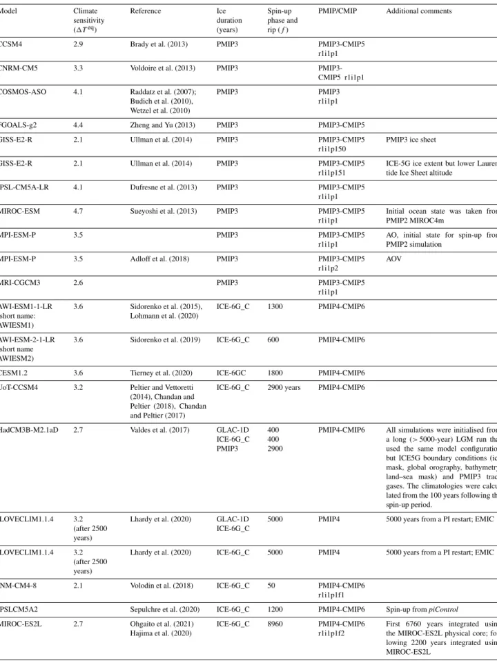
Table 1.PMIP3 and PMIP4 models analysed in the present study. The spin-up duration is only given for the new PMIP4-CMIP6 models.
Model Climate Reference Ice Spin-up PMIP/CMIP Additional comments sensitivity duration phase and
(1Teq) (years) rip (f )
CCSM4 2.9 Brady et al. (2013) PMIP3 PMIP3-CMIP5 r1i1p1
CNRM-CM5 3.3 Voldoire et al. (2013) PMIP3 PMIP3-CMIP5 r1i1p1 COSMOS-ASO 4.1 Raddatz et al. (2007);
Budich et al. (2010), Wetzel et al. (2010)
PMIP3 PMIP3
r1i1p1
FGOALS-g2 4.4 Zheng and Yu (2013) PMIP3 PMIP3-CMIP5
GISS-E2-R 2.1 Ullman et al. (2014) PMIP3 PMIP3-CMIP5 r1i1p150
PMIP3 ice sheet
GISS-E2-R 2.1 Ullman et al. (2014) PMIP3 PMIP3-CMIP5 r1i1p151
ICE-5G ice extent but lower Lauren-tide Ice Sheet altitude
IPSL-CM5A-LR 4.1 Dufresne et al. (2013) PMIP3 PMIP3-CMIP5 r1i1p1 MIROC-ESM 4.7 Sueyoshi et al. (2013) PMIP3 PMIP3-CMIP5
r1i1p1
Initial ocean state was taken from PMIP2 MIROC4m
MPI-ESM-P 3.5 PMIP3 PMIP3-CMIP5
r1i1p1
AO, initial state for spin-up from PMIP2 simulation
MPI-ESM-P 3.5 Adloff et al. (2018) PMIP3 PMIP3-CMIP5 r1i1p2
AOV
MRI-CGCM3 2.6 PMIP3 PMIP3-CMIP5
r1i1p1 AWI-ESM1-1-LR (short name: AWIESM1) 3.6 Sidorenko et al. (2015), Lohmann et al. (2020) ICE-6G_C 1300 PMIP4-CMIP6 AWI-ESM-2-1-LR (short name AWIESM2)
3.6 Sidorenko et al. (2019) ICE-6G_C 600 PMIP4-CMIP6
CESM1.2 3.6 Tierney et al. (2020) ICE-6GC 1800 PMIP4-CMIP6
UoT-CCSM4 3.2 Peltier and Vettoretti (2014), Chandan and Peltier (2018), Chandan and Peltier (2017)
ICE-6G_C 2900 years PMIP4-CMIP6
HadCM3B-M2.1aD 2.7 Valdes et al. (2017) GLAC-1D ICE-6G_C PMIP3
400 400 2900
PMIP4-CMIP6 All simulations were initialised from a long (> 5000-year) LGM run that used the same model configuration but ICE5G boundary conditions (ice mask, global orography, bathymetry, land–sea mask) and PMIP3 trace gases. The climatologies were calcu-lated from the 100 years following the spin-up period.
iLOVECLIM1.1.4 3.2 (after 2500 years)
Lhardy et al. (2020) GLAC-1D ICE-6G_C
5000 PMIP4 5000 years from a PI restart; EMIC
iLOVECLIM1.1.4 3.2 (after 2500 years)
Lhardy et al. (2020) ICE-6G_C 5000 PMIP4 5000 years from a PI restart; EMIC
INM-CM4-8 2.1 Volodin et al. (2018) ICE-6G_C 50 PMIP4-CMIP6 r1i1p1f1
IPSLCM5A2 Sepulchre et al. (2020) ICE-6G_C 1200 PMIP4-CMIP6 Spin-up from piControl
MIROC-ES2L 2.7 Ohgaito et al. (2021) Hajima et al. (2020)
ICE-6G_C 8960 PMIP4-CMIP6 r1i1p1f2
First 6760 years integrated using the MIROC-ES2L physical core; fol-lowing 2200 years integrated using MIROC-ES2L
MPI-ESM1.2 2.77 Mauritsen et al. (2019) ICE-6G_c 3850 PMIP4-CMIP6 r1i1p1f1
3850 years after restart from a previ-ous lgm simulation.
total of 13 PMIP4 LGM simulations are currently available and slightly more than the 11 LGM simulations in PMIP3 (Table 1). The PMIP3 ensemble includes one model that ran an additional sensitivity test to ice-sheet height (GISS-E2R; Ullman et al., 2014) and one model that ran simu-lations with and without dynamic vegetation (MPI-ESM-P; Adloff et al., 2018). The PMIP4-CMIP6 ensemble includes three simulations made with updated versions of the mod-els that contributed to PMIP3-CMIP5, specifically IPSLCM, MIROC and MPI-ESM (Table 1). However, the IPSL simu-lation for PMIP4 does not use the latest IPSLCM6 version specifically developed for CMIP6 due to the impossibility to run the lgm experiment with this version. Most of the models that have run the PMIP4-CMIP6 LGM simulations are general circulation models (GCMs) but iLOVECLIM is an Earth system model of intermediate complexity, which is considerably faster than the GCMs. The iLOVECLIM and the HadCM3B-M2.1aD GCMs are the only models in the en-semble to have run simulations using different ice-sheet re-constructions (both models ran with ICE-6G_C and GLAC-1D, and HadCM3B-M2.1aD also ran with the PMIP3 ice sheet). The LGM simulations were either initialised from a previous LGM simulation or were spun up from the pre-industrial state. The length of the spin-up therefore varies (Table 1), as does the length of the equilibrium LGM sim-ulation in these preliminary analyses. The INM-CM4-8 re-sults are from the beginning of an lgm simulation and the model is not yet fully equilibrated. All other models have run for several millennia. Our preliminary analyses are based on variables available by 14 December 2020. Although several of the PMIP4-CMIP6 models have higher climate sensitiv-ity than the equivalent models in PMIP3-CMIP5, this is not reflected in the ensemble analysed here. In fact, the PMIP4-CMIP6 ensemble, as of December 2020, has lower climate sensitivities than the PMIP3-CMIP5 models (Table 1): equi-librium sensitivities to a CO2 doubling from pre-industrial
values range from 2.1 to 3.6◦C, (mean: 3.0◦C) in the cur-rent PMIP4-CMIP6 ensemble, while the range is from 2.1 to 4.7◦C (mean: 3.4◦C) in the PMIP3-CMIP5 ensemble.
All in all, only a minority of models present in the PMIP3 ensemble ran the PMIP4 simulation, so that the PMIP4 en-semble differs from the PMIP3 one because of the update of these models but mostly because it gathers new models com-pared to PMIP3. This adds up to the change in protocol from PMIP3 to PMIP4 to explain differences in model results be-tween these two phases of PMIP.
2.3 Sources of information on LGM climate
The PMIP3-CMIP5 model simulations were evaluated against two benchmark datasets: pollen-based reconstruc-tions of seasonal temperature (mean annual temperature – MAT, mean temperature of the coldest month – MTCO, mean temperature of the warmest month – MTWA, growing season temperature indexed by growing degree days above
a baseline of 0◦C), mean annual precipitation (MAP) and an index of soil moisture (Bartlein et al., 2011); and a com-pilation of sea-surface temperature (SST) reconstructions (MARGO Project Members, 2009).
In the Bartlein et al. (2011) dataset, reconstructions at in-dividual pollen sites were averaged to produce an estimate for a 2 × 2◦grid; reconstruction uncertainties are estimated as a pooled estimate of the standard errors of the original reconstructions for all sites in each grid cell. Although the Bartlein et al. (2011) dataset has good coverage for some re-gions, coverage was sparse in the tropics, and there were no reconstructions of LGM climate for Australia. Furthermore, not all of the six climate variables were reconstructed at ev-ery site, so statistical comparisons were more robust for some variables than others. The majority of the reconstructions in-cluded in the Bartlein et al. (2011) dataset used various sorts of statistical calibrations based on modern-day conditions and therefore do not account for the impact that changes in CO2 have on water-use efficiency and hence plant
distribu-tion. Although Bartlein et al. (2011) were unable to demon-strate a statistically significant difference between statistical reconstructions and model-based inversions (which, in prin-ciple, account for the CO2effect on plant distribution), their
analysis focused on the mid-Holocene where the CO2effect
is small. There is therefore some concern that the dataset may overestimate aridity at the LGM. Reconstructions which in-corporate the effect of CO2are now available for Australia
(Prentice et al., 2017). Cleator et al. (2020) have used 3-D variational data assimilation techniques with a prior derived from the PMIP3-CMIP5 LGM simulations and the Bartlein et al. (2011) and Prentice et al. (2017) pollen-based recon-structions, and incorporating the Prentice et al. (2017) CO2
correction, to produce a new global reconstruction of terres-trial climate at the LGM. In addition to accounting for poten-tial effects of low CO2on moisture variables at the LGM, this
reconstruction produces coherent estimates of seasonal cli-mate variables at many more points than the original pollen-based reconstructions and also extends the geographic cov-erage.
Tierney et al. (2020) provide a new synthesis of geochem-ical SST data (UK370, TEX86, Mg/Ca and δ18O) from the
LGM (defined as the period from 19 000 to 23 000 years ago) and the late Holocene (defined as the period from 4000 years ago to the present) time periods. This compilation builds upon the MARGO Project Members (2009) collec-tion of UK370 and Mg/Ca data by including new studies pub-lished since MARGO was released, as well as expanding the collection to include TEX86 and δ18O of foraminifera.
The Tierney et al. (2020) synthesis excludes microfossil-based SST estimates, on the basis that these (1) include no-analogue assemblages (Mix et al., 1999); (2) imply warmer-than-present subtropical gyres, an inference that has been questioned (Crowley, 2000; Telford et al., 2013); and (3) lack Bayesian proxy-system models that were required for the data assimilation technique used by Tierney et al. (2020).
Tierney et al. (2020) use the data along with a model prior from the isotope-enabled Community Earth System Model 1.2 (CESM1.2; Brady et al., 2019) to produce a full-field data assimilation product. Here, we use both the data syn-thesis and the data assimilation products, labelled “Tier-ney2020” and “Tierney2020DA”, respectively. Data from the LGM and late Holocene, respectively, were calibrated using Bayesian models that fully propagate uncertainties (Tierney and Tingley, 2015; Tierney et al., 2018, 2019; Malevich et al., 2019), yielding a 1000-member posterior distribution of SSTs. These data were sorted from low to high along the en-semble dimension, and then random error representative of site-level downcore uncertainty following the Gaussian dis-tribution N (0, 0.5◦C) was added back to the matrix. This procedure effectively partitions the error variance; i.e. it as-sumes that at any given site, absolute uncertainty in SST cancels out in the anomaly calculation, while “relative” un-certainty associated with downcore measurement and non-linearities in the calibration model is preserved. The data were then averaged within a 5◦×5◦ grid and differenced. The standard deviation associated with each grid point is cal-culated from the differenced ensemble dimension.
In the present work, we also use other available recon-structions, all based on at least part of the initial MARGO Project Members (2009) reconstructions at the core sites: all are global reconstructions, obtained from this dataset via dif-ferent methods, as summarised by Paul et al. (2021). These datasets are from
– Annan and Hargreaves (2013), who use the MARGO Project Members (2009) dataset, the Bartlein et al. (2019) reconstructions on the continents, as well as the PMIP2 model output to generate a reconstruction of the sea-surface temperatures using multiple linear re-gression;
– Kurahashi-Nakamura et al. (2017), who use the MARGO Project Members (2009) data, benthic δ18O and δ13C data as well as the MIT General Circula-tion Model (MITgcm) in combinaCircula-tion with the method of Lagrange multipliers/adjoint method to generate a global reconstruction;
– Paul et al. (2021), who produced the GLOMAP2020 dataset based on the floral and faunal assemblage data, as well as various sea-ice reconstructions from MARGO Project Members (2009), together with an op-timal gridding method called DIVA to produce monthly global reconstructions. A caveat given in Paul et al. (2021) about this reconstruction is that it may be too warm by 0.5 to 1.0◦C due to impacts of changes in sea-sonality and in the thermal structure of the ocean that are not taken into account in their reconstructions, as well as the impact due to heterogeneous spatial sampling. These datasets reflect different approaches and choices of initial datasets (only geochemical data for the Tierney et
al. (2020) reconstructions, for which the sites are often close to the coasts or only floral and faunal assemblages for GLOMAP2020), which yields a range a results with illustrate the uncertainty of the SST reconstructions. A crucial differ-ence between the Tierney et al. (2020) synthesis and the other datasets used here is that the former implies more exten-sive tropical cooling during the LGM (−2.5◦C vs. −1.5◦C for MARGO, −1.2◦C for GLOMAP2020, −1.6◦C for An-nan and Hargreaves, 2013, −1.7◦C for Kurahashi-Nakamura et al., 2017). This can be attributed to the exclusion of the microfossil data as well as recalibration of the UK370 proxy with the BAYSPLINE model (Tierney and Tingley, 2018), which corrects for an observed reduced sensitivity of UK370 to SST above approximately 24◦C. The data-assimilated prod-uct from Tierney et al. (2020) is even cooler, which might be related to the choice of the global model for the assimilation. A further comparison is presented in Paul et al. (2021).
2.4 Data–model comparisons
We compare the model simulations to paleoclimate data, fo-cusing on large-scale features and regional changes. In these comparisons, the reconstructions are expressed as mean val-ues and the uncertainty by the standard error of the recon-structions. Model outputs were extracted only for the grid cells where there are observations. Model uncertainty is rep-resented by the standard deviation of 10 000 averages over 50 years randomly picked in the ≥ 100-year-long time se-ries of model outputs. Thus, model uncertainty is not, strictly speaking, equivalent to reconstruction uncertainty but merely provides some measure of the variability engendered by sam-pling the simulated climate.
3 Model results
3.1 Temperature
The global and annual mean temperature in the PMIP4 LGM simulations is between 3.3 and 7.2◦C cooler than the PI sim-ulations (Fig. 1, Table S1). The largest changes in tempera-ture between the LGM and PI simulations (Fig. 2) are found over the Laurentide and Fennoscandian ice sheets, reflecting the significant changes in surface height and albedo caused by the ice sheets. Colder conditions are registered in the northern midlatitudes and high latitudes, partly reflecting the advection of the cold temperature anomalies downwind of the ice sheets. The cooling in the tropics, which results from both the lower atmospheric GHG concentrations and the re-mote influence of the northern ice sheets, is more muted. As expected, the simulations show larger changes over the land than over ocean. The ratio between the LGM–PI mean sur-face air temperature anomaly over land and the anomaly over the ocean ranges from 1.0 to 1.6 over the tropics (30◦S to 30◦N) and from 1.90 to 5.5 for globally averaged tempera-tures. Zonally averaged temperatures (Fig. 1a) confirm that
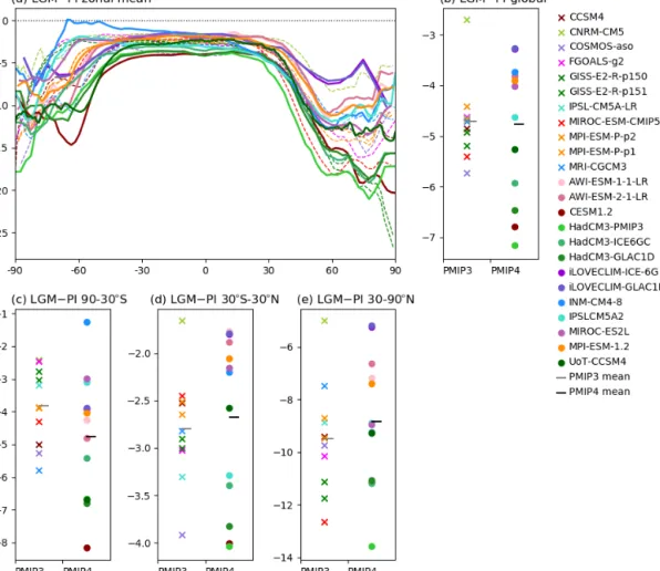
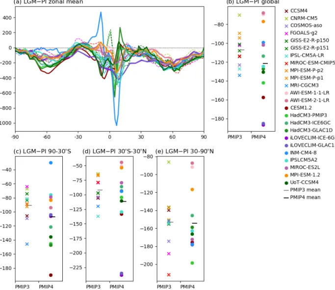
Figure 1.Mean annual surface air temperatures LGM–PI anomalies in◦C. (a) Zonal means, PMIP3 model results shown as dashed lines, PMIP4 model results shown as thick solid lines; (b) global means, PMIP3 model results shown by crosses, PMIP4 models shown by filled circles; averages over (c) the southern extratropics (90 to 30◦S), (d) the tropics (30◦S to 30◦N) and (e) the northern extratropics (30 to 90◦N).
the PMIP4 ensemble also shows the expected polar ampli-fication of temperature changes in both the Northern Hemi-sphere and Southern HemiHemi-sphere.
Although the broad-scale patterns of temperature changes are similar, there are differences between the PMIP4 and PMIP3 ensembles. The PMIP4 ensemble average is warmer than the PMIP3 ensemble average (Fig. 2 bottom) over North America, south of the ice sheet, over the Labrador and Nordic Seas and the Tibetan Plateau. On the other hand, the PMIP4 average is colder than the PMIP3 one in regions close to West Antarctica, over some areas of the Laurentide Ice Sheet, over the marine part of the Fennoscandian Ice Sheet and in the North Atlantic and the northern part of the North Pacific. The largest difference between the PMIP3 and PMIP4 av-erages is over the northern North Atlantic and Nordic Seas, probably reflecting differences in sea-ice cover in these ar-eas. Zonally averaged temperatures (Fig. 1a) show that the
PMIP4 global mean annual temperature LGM–PI anomalies spread over a larger range than the PMIP3 ensemble, with a few PMIP4 models (in particular the three HadCM3 simula-tions and CESM1.2) showing larger cooling than the cold-est PMIP3 models. Nonetheless, the multi-model average of the global mean annual temperature LGM–PI anomalies are similar for both ensembles (−4.71◦C for the PMIP3 ensem-ble, −4.77◦C for the PMIP4 ensemble; see Supplement Ta-ble S1).
The northern extratropics are slightly colder in the PMIP3 simulations (multi-model LGM–PI MAT anomaly of −9.5◦C) than in the PMIP4 simulations (multi-model aver-age of −8.8◦C). The minimum cooling and maximum cool-ing over the PMIP3 and PMIP4 ensembles are also very simi-lar. The PMIP3 and PMIP4 simulations yield similar cooling in the tropics (multi-model average of −2.8◦C for the PMIP3 ensemble and of −2.7◦C for the PMIP4 ensemble, with
simi-Figure 2.LGM mean annual temperature (in◦C) simulated by the ensemble of PMIP4 models (a), LGM–PI mean annual temperature anomaly (in◦C) simulated by the same models (middle, where stip-pling shows where models do not agree on the sign of changes), difference between the PMIP4 and PMIP3 ensembles (in ◦C, b). The PMIP4 average is based on models listed in Table 1, except for iLOVECLIM simulations, which are at lower resolution. The PMIP3 average is based on all PMIP3 models, except the GISS-E2-p151 simulation, which did not use the PMIP3 ice sheet for its boundary conditions.
lar minima and maxima; see Table S1). However, the cooling of the southern extratropics is more variable in the PMIP4 simulations (−1.2 to approximately −8.15◦C) than in the PMIP3 simulations (−2.4 to approximately −5.8◦C), and its multi-model average is larger for the PMIP4 ensemble (−4.8◦C, compared to −2.8◦C for the PMIP3 ensemble).
Therefore, most of the difference in the global average cool-ing, which ranges from −3.3 to −7.2◦C in the PMIP4 sim-ulations and between −2.7 and −5.7◦C in the PMIP3 simu-lations, stems from differences in the simulated temperatures over the Southern Hemisphere. It is difficult to assign these differences between the PMIP3 and PMIP4 ensembles to a single reason, since both models and protocols have changed
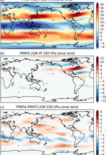
Figure 3.Same as Fig. 2 but for the 250 hPa zonal wind. The PMIP4 average is based on all models listed in Table 1. The PMIP3 average is based on all PMIP3 models in Table 1, except the GISS-E2-p151 simulation, which did not use the PMIP3 ice sheet for its boundary conditions.
between these two phases. Sensitivity experiments and in-depth study of the experiments carried out with the PMIP3 and PMIP4 protocols but with the same models will be nec-essary to disentangle the reasons for the differences between the PMIP3 and PMIP4 results. It is in fact rather intriguing that the average cooling over the North American ice sheet is larger in the PMIP4 ensemble, given that both the ICE-6G_C and the GLAC-1D reconstructions yield significantly lower altitudes than the PMIP3 ice-sheet reconstruction, used in all the PMIP3 experiments.
3.2 Atmospheric and oceanic circulation
The PMIP4-CMIP6 models simulate large changes in the Northern Hemisphere upper tropospheric atmospheric circu-lation (Fig. 3), in response to LGM boundary conditions, in particular over North America and the North Atlantic. The North Atlantic jet stream is narrower and stronger com-pared to the PI, as shown by an increase reaching more than
10 m s−1 in the 250 hPa zonal wind south of the Lauren-tide Ice Sheet and extending into the North Atlantic, and a decrease in zonal wind to the northwest and southeast of these regions. The strengthening and narrowing of the North Atlantic jet stream was also a characteristic of the PMIP3-CMIP5 simulations (Beghin et al., 2016). However, in the PMIP4-CMIP6 simulations, the jet stream extends further north than in the PMIP3 simulations (Fig. 3, bottom), most prominently near the Laurentide Ice Sheet. This could be be-cause the Laurentide Ice Sheet is lower in the ICE-6G recon-struction than the ice sheet used in the PMIP3-CMIP5 sim-ulations (see, e.g. Ullman et al., 2014; Beghin et al., 2015; Lofverstom et al., 2016) but may also reflect changes in the representation of the zonal winds between the two sets of simulations. This is supported by the fact that there are dif-ferences between the PMIP3-CMIP5 and PMIP4 simulations away from the Laurentide Ice Sheet, in particular over the Southern Ocean, where the jet stream is also located more poleward in the PMIP4 than the PMIP3 simulations. Sensi-tivity experiments using the PMIP3-CMIP5 ice sheets with PMIP4 models, as planned in the PMIP4 LGM experiment protocol (Kageyama et al., 2017), should help resolve the question of whether differences in model treatment or bound-ary conditions are responsible for the differences in atmo-spheric circulation between the two ensembles.
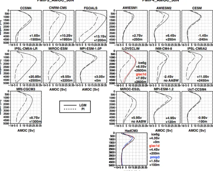
The extent of the NADW cell (identified in Fig. 4 by the depths for which the Atlantic meridional overturning streamfunction at 30◦N is positive) simulated by PMIP4 models is very similar for LGM and PI, except for iLOVE-CLIM and IPSLCM5A2, which show a very large deepening of the NADW cell for LGM (Fig. 4). Two of the PMIP4-CMIP6 models (INM-CM4-8 and MIROC-ES2L) show a deep NADW cell reaching the ocean floor in the North At-lantic, whereas five of the PMIP4-CMIP6 models (MPI-ESM1.2, UoT-CCSM4, AWIESM2, C(MPI-ESM1.2, HadCM3) simulate a clear AABW in the North Atlantic. UoT-CCSM4 and CESM1.2 even shows a shallowing of the NADW cell for LGM. The intrusion of AABW cell (defined by nega-tive values in the Atlantic meridional overturning stream-function at 30◦N) into the North Atlantic was shown by some of the PMIP3-CMIP5 simulations (CCSM4, MPI-ESM-1.0P) but not as much as the PMIP4 simulations (AW-IESM2, CESM1.2, MPI-ESM-1.2, UoT-CCSM4 and the three HadCM3 simulations, Fig. 4 and Muglia and Schmit-tner, 2015). Five of the PMIP3-CMIP5 models produced a NADW cell reaching the ocean floor in the North At-lantic and only two had extensive AABW. The maximum strength of the NADW cell itself strengthens in all of the PMIP4 simulations by as much as 11 Sv for IPSLCM5A2. This strengthening is consistent with PMIP3-CMIP5 results and is likely to be associated with the vigorous surface wind over the northern North Atlantic (Muglia and Schmittner, 2015; Sherriff-Tadano and Abe-Ouchi, 2020) and the closure of the Bering Strait (Hu et al., 2015). The strength of the AMOC reduces south of 30◦N in UoT-CCSM4 (see
Sup-plement Fig. S2). iLOVECLIM performed simulations of LGM with two different ice-sheet reconstructions (ICE6G, GLAC1D) and shows a weaker NADW cell in GLAC-1D than that produced by ICE-6G_C (Fig. 4). This weakening is likely to be associated with a lower topography of the ice sheet of GLAC1D (e.g. Zhang et al., 2014). On the other hand, HadCM3 was used with the PMIP3, ICE-6G_C and GLAC-1D ice sheets, and the results in terms of AMOC are very similar for the ICE-6G_C and GLAC-1D ice sheets, for which the AMOC slightly strengthens compared to PI, while the AMOC is similar to the PI one for the simulation using the PMIP3 ice sheet.
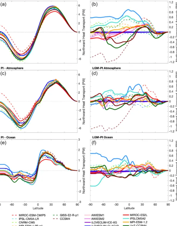
These circulation changes in the Atlantic Ocean are re-flected in the total ocean heat transport (Fig. 5, bottom, the PMIP4 results available for this analysis are from all ulations but the HadCM3 simulations). MPI-ESM1.2 sim-ulates an increase in northward ocean heat transport at all latitudes for the LGM compared to PI, while MIROC-ES2L simulates an increase in this transport from 15◦S to 60◦N. UoT-CCSM4 and CESM1.2 are the only models simulating a decrease in northward heat transport over a significant range of latitudes, from 50◦S to 70◦N, in the lgm run compared to the piControl one. INCM4-CM4-8 simulates increased ocean transport south of 20◦N. IPSLCM5A2’s ocean transport de-creases south of 30◦S and between the Equator and 30◦N but significantly increases in the southern tropics. All PMIP4 models simulate an increase in northward atmospheric heat transport, in the tropics and up to 50◦N, in the lgm simula-tion compared to piControl. MIROC-ES2L simulates an in-crease up to 70◦N (Fig. 5, middle). In summary, all models simulate an increase, in their lgm run compared to piCon-trol, in northward heat transport (Fig. 5, top) in the tropics and northern midlatitudes, although in the UoT-CCSM4 and CESM1.2 models the increase is confined between ∼ 10 and 50◦N. This increase in northward heat transport in the tropics and northern midlatitudes during the LGM as compared to PI was also simulated by most PMIP3-CMIP5 models. Given that the magnitude of the heat transport increase is similar in the PMIP4 and PMIP3-CMIP6 simulations, the warmer temperatures at high northern latitudes in the PMIP4-CMIP6 simulations cannot be due to differences in northward ocean heat transport.
3.3 Hydrological cycle
The large-scale gradients in precipitation are similar in the multi-model average of the PMIP4 LGM and PI simulations (Fig. 6, top left), with maximum precipitation in the trop-ics (Intertropical Convergence Zone (ITCZ) and monsoon regions) and secondary maxima in the midlatitudes, corre-sponding to the position of the North Pacific, North Atlantic and Southern Ocean storm tracks. The PMIP4 models show a decrease in precipitation between the LGM and PI in all these high-precipitation areas (Fig. 6, bottom left and Fig. 7, top left). There are some regions where precipitation increases
Figure 4.Mean Atlantic Meridional Overturning Circulation (mean meridional stream function for the Atlantic Ocean at 30◦N) simulated by the PMIP3 and PMIP4 models for PI and LGM. Numbers in Sv indicate the LGM–PI anomaly in terms of maximum Atlantic meridional overturning streamfunction. Numbers in metres indicate the LGM–PI anomaly in terms of NADW vertical extension, the NADW vertical extent being defined here as the depths over which the mean meridional stream function for the Atlantic Ocean at 30◦N is positive.
during the LGM compared to the PI: at least nine PMIP4 models (as shown by the areas which are not stippled) show more precipitation over the subtropical Pacific Ocean and to the south of the Laurentide Ice Sheet, over southern Africa and over the Iberian Peninsula, and some simulate an in-crease in precipitation over the northern and southern sub-tropical zones in the Pacific and over the southern subsub-tropical zone in the Atlantic. However, the areas with decreased pre-cipitation are much more extensive than areas with increased precipitation, so zonal averages for the southern extratropics, tropics and northern extratropics (Fig. 7) all show a decrease in precipitation.
The broad-scale patterns of change in precipitation in the PMIP4 simulations are similar to those found in the PMIP3-CMIP5 simulations (Fig. 7, top left). However, the PMIP4 multi-model average is drier than the PMIP3-CMIP5 one (Fig. 6) at the global scale as well as for the southern
ex-tratropics and for the tropics. It is similar for both ensembles for the northern extratropics. The geographic patterning in the precipitation changes between the PMIP4 and PMIP3-CMIP5 ensembles (Fig. 6, top right) are complex, particu-larly in the tropical where the wetter–drier–wetter pattern in the meridional direction suggests differences in ITCZ rep-resentation between the two generations of models. This is confirmed by the same figure drawn for the PI (Fig. 6, bot-tom right), which shows very similar patterns in the PMIP3 vs. PMIP4 anomalies. Both ensembles show a consistent decrease in zonally averaged precipitation in the southern and northern extratropics (Fig. 7). As for the mean annual temperature, the simulated range of precipitation changes is larger for PMIP4 ensemble compared to the PMIP3 one, ex-cept for the northern extratropics for which both ensembles show a similar range (Figs. 7 and 2).
Figure 5.Meridional energy transport for the PI reference state (left-hand side) and LGM–PI anomaly (right-hand side). (a, b) Total energy transport, (c, d) atmospheric energy transport, (e, f) oceanic energy transport.
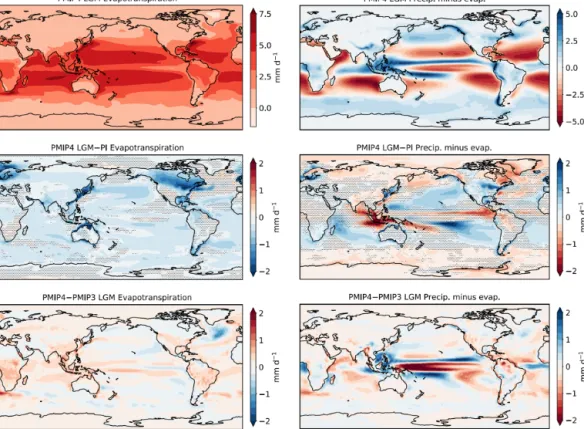
Evapotranspiration patterns in the PMIP4 LGM and PI simulations are characterised by maximum values in the sub-tropics and decrease towards high latitudes. The models sim-ulate a global decrease in LGM evapotranspiration relative to the PI that strongly peaks over and around the North-ern Hemisphere ice sheets (Fig. 8, left). These results are in agreement with the broad patterns of the PMIP3-CMIP5
en-semble, except for a stronger decrease in evaporation in the northern North Atlantic, which corresponds to the larger av-erage cooling in these regions in the PMIP4 ensemble com-pared to the PMIP3 ensemble. As a result, net precipitation (precipitation minus evapotranspiration) in the PMIP4 en-semble is higher during the LGM than the PI in the extra-tropics – particularly over the midlatitude eastern Pacific in
Figure 6.(a, b) PMIP4-CMIP6 multi-model LGM mean annual precipitation in mm d−1. (c) PMIP4-CMIP6 multi-model LGM–PI mean annual precipitation anomaly (mm d−1) with stippling showing areas where less than nine models agree on the sign of change. (b) Difference between the PMIP4-CMIP6 and the PMIP3 multi-model means of the LGM mean annual precipitation (mm d−1). (d) Difference between the PMIP4-CMIP6 and the PMIP3 multi-model means of the PI mean annual precipitation (mm d−1).
both hemispheres and over most of North America – with the exception of the North Atlantic, where evaporation decreases are more localised and do not compensate for the reductions in precipitation (Fig. 8, right). This, together with colder tem-peratures, could help explain why the PMIP4 models simu-late a stronger AMOC at the LGM. Substantial reductions in continental net precipitation only occur over tropical South America and high-latitude regions, over the Labrador Sea and its surrounding ice sheets, while Africa, Australia and the midlatitude regions of Eurasia and the Americas see little change or even increased net precipitation.
4 Data–model comparisons
The evaluation of the PMIP3-CMIP5 LGM simulations showed that large-scale climate features, such as the ratio of changes in land–sea temperature, high-latitude tempera-ture amplification and precipitation scaling with temperatempera-ture, were broadly consistent with modern observations (Bracon-not et al., 2012; Izumi et al., 2013; Harrison et al., 2014, 2015).
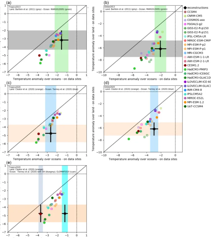
All PMIP3 and PMIP4 models simulate larger cooling over land than over oceans, on average for the tropics and for the globe. Figure 10 shows averages of model output sam-pled at sites for which there are reconstructions compared to the averages of the reconstructed values. Since the differ-ent reconstructions do not cover the same sites, the averages of the model values at reconstruction sites differ slightly for each dataset. However, for all datasets, the multi-model rela-tionship between the average cooling over land and that over the ocean is approximately linear. Figure 10 allows a com-parison between model output and reconstructions averaged
over land and over oceans, as well as a comparison of the ratio of the land cooling over the ocean cooling. Although the Cleator et al. (2020) dataset has a larger spatial coverage than the Bartlein et al. (2011) dataset, there is no significant difference between the two datasets for most of the temper-ature variables across common grid cells (Fig. 9). However, the new reconstructions have a reduced range at the warm end, especially between 0 and 40◦N, so that for the averages over the tropics, most simulations are recorded as within or warmer than the land-based reconstructions, while they are within or colder than the Bartlein et al. (2011) reconstruc-tions (Fig. 10, left-hand side). The results for the global aver-ages are fairly consistent for both land-based reconstructions (Fig. 10, right-hand side) but the uncertainty is smaller for the Cleator et al. (2020) dataset. All in all, there are as many sim-ulations within the range of globally averaged reconstructed temperatures of Cleator et al. (2020) as that of Bartlein et al. (2011) but the models outside this range tend to be on the warm side for the Cleator et al. (2020) dataset and both on the warm and cold sides for the Bartlein et al. (2011) dataset. The reconstructions of the LGM–Late Holocene SST anomalies provided by Tierney et al. (2020) are colder than the MARGO reconstructions in the tropics, and although this removes the apparent cold-bias shown by some simulations, this results in some simulations falling outside the window of reconstructed SSTs at the warm end. This is even more the case if we compare the results to the data-assimilated prod-uct from Tierney et al. (2020), which has a global coverage (Fig. 10, left-hand side, bottom line). The results from this latter dataset contrast the results from other global products, as shown in Supplement Fig. S3. These other global datasets (Annan and Hargreaves, 2013; Kurahashi-Nakamura et al.,
Figure 7.Same as Fig. 1 for mean annual precipitation in mm yr−1.
2017; GLOMAP2020 from Paul et al., 2021) are all derived, at least in part, from the MARGO Project Members (2009) dataset, which might explain their overall consistency with the averages estimated by MARGO Project Members (2009). We have added the warmest estimate (GLOMAP2020) which includes uncertainties in Fig. 10 to obtain a more complete view of the available reconstructions as of 2020, keeping in mind that the authors of the GLOMAP2020 reconstruction estimate that it could be biased by 0.5 to 1.0◦C in the trop-ics. The simulated mean annual surface air temperature de-creases over the tropical oceans stand between these two ex-tremes. This illustrates that model-related uncertainties are comparable with the uncertainties raising from the multi-ple approaches taken to reconstruct both the continental and oceanic temperatures.
The ratio for the land–sea difference in changes in mean annual temperature in the tropics in the PMIP4 simula-tions is compatible with the ratio reconstructed from the Bartlein et al. (2011) and MARGO Project Members (2009) datasets. This is also the case if we consider the more re-cent reconstructions by Cleator et al. (2020) and Tierney et al. (2020), although the multi-model land–sea ratio ap-pears to be smaller than that suggested by the reconstruc-tions. This is the case for both the tropical and global av-erages. However, it would not be compatible with a land– sea contrast based on the Cleator et al. (2020) dataset and the GLOMAP2020 dataset, even if the warm bias pointed by its authors is taken into account. We are therefore left with large uncertainties on the topic of LGM cooling over land and oceans, from the reconstructions as well as from the models. The uncertainties based on the ensemble of model results and
Figure 8.Same as Fig. 2 for mean annual evaporation (left-hand side) and mean annual net precipitation (precipitation–evaporation, right-hand side). All values are in mm d−1. Stippling shows areas where less than nine models agree on the sign of change.
on the ensemble of continental and marine reconstructions are actually very similar.
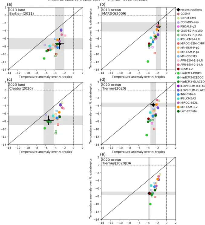
The amplification of temperature changes at high north-ern latitudes compared to the tropics is apparent over both the land and the ocean domains, although the amplification appears to be smaller in the new data syntheses (Fig. 11), except of the Tierney et al. (2020) data-assimilated product. For the ocean domain, this could reflect the influence of sea-sonal production on the extratropical sites, with indicators being more sensitive to summer changes or to changes in the seasonal production cycle. Comparisons of the amplification over land areas with the Bartlein et al. (2011) dataset sug-gest that the simulated tropical cooling is too large in the PMIP3-CMIP5 simulations, whereas the extratropical cool-ing was both larger and smaller than that suggested by the re-constructions in both ensembles. Simulated tropical temper-atures are more consistent with or warmer than the Cleator et al. (2020) reconstructions, suggesting that the apparent over-estimation of tropical cooling in the PMIP3-CMIP5 simula-tions over land may reflect the paucity of tropical data points in Bartlein et al. (2011). However, the discrepancies between the simulated and reconstructed extratropical land temper-atures are still present: there are several PMIP3 and PMIP4 simulations that are much colder than the reconstructions and many which are warmer than the reconstructions. Although polar amplification is more muted over the ocean domain, the
comparisons show a similar picture to the land-based com-parisons. Simulated tropical ocean temperatures are more compatible with the Tierney et al. (2020) than the MARGO Project Members (2009) synthesis. Simulated extratropical temperature changes in the PMIP3-CMIP5 ensemble mean are considerably colder than those shown by either of these syntheses, but most tend to be on the warm side of the Tier-ney et al. (2020) data-assimilated product.
The LGM climate is characterised by an increase in tem-perature seasonality in extratropical regions, with larger changes in winter than in summer (Izumi et al., 2013). This is confirmed by the Cleator et al. (2020) reconstructions. In general, this change in seasonality is reproduced by the mod-els, although the ranges of PMIP4 results for winter are less distinct from their summer counterparts than for the PMIP3 models. The multi-model average seasonality is, however, in-creased for both ensembles. The simulated cooling in winter temperature is smaller than that indicated by the Bartlein et al. (2011) reconstructions (Fig. 12, top line). This is not the case compared to the Cleator et al. (2020) reconstructions, with which more models are in agreement, except for western Europe, which remains a region of model–data discrepancy. The magnitude of the summer cooling is more consistent be-tween the PMIP4 simulations and the Cleator et al. (2020) reconstructions than between the PMIP3 simulations and the Bartlein et al. (2011) reconstructions in North America,
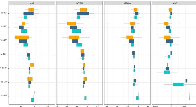
Eu-Figure 9.Comparison of terrestrial climate variables from the combined Bartlein et al. (2011) and Prentice et al. (2017) dataset and from the Cleator et al. (2020) reconstruction using data assimilation, averaged over 20◦latitudinal bands. The variables are mean annual temperature (MAT), mean temperature of the coldest month (MTCO), mean temperature of the warmest month (MTWA) and mean annual precipitation (MAP). The orange boxplots show the results from the Bartlein et al. (2011) and Prentice et al. (2017) combined dataset, the dark blue boxplots for the reconstructions by Cleator et al. (2020) at sites for which there are reconstructions in the combined dataset, and the green boxplots show the results for the full reconstructions from Cleator et al. (2020).
rope and extratropical Eurasia. Finally, the North Atlantic mean annual cooling simulated by the PMIP4 models spans a larger range that of the PMIP3 ensemble. While the PMIP3 ensemble mean showed temperatures within or above the re-constructed ranges from all oceanic datasets, the PMIP4 en-semble average stands within the range of the reconstruc-tions, with six individual models being within this range, four above and three below. It is therefore quite difficult to deter-mine the cause of the discrepancy in western Europe winter temperatures, which was previously assigned to an underes-timation of the North Atlantic cooling. Some of the PMIP4 simulations are in fact much colder over both the North At-lantic and western Europe, and could be studied to further disentangle this model–data disagreement.
Regional changes in the tropics (Fig. 12, bottom line) are more muted than those in the northern extratropics, and sea-sonality differences are small. We therefore base our com-parisons on the mean annual temperature and mean annual precipitation. Both PMIP3 and PMIP4 multi-model averages underestimate MAT cooling over tropical America, which is consistent for both reconstructions. More PMIP4 results stand within the reconstructed range over tropical America. Over tropical Africa, the PMIP3 models were broadly con-sistent with the Barltein et al. (2011) reconstructed MAP anomaly but underestimate this cooling if we refer to the
more recent Cleator et al. (2020) reconstructions. This is also the case for the PMIP4 models, but four simulations (IPSLCM5A2 and the three HadCM3 simulations) are now within the reconstructed range. This is probably related to the simulated tropical SSTs being colder in these simula-tions. The reconstructed changes in tropical precipitation over America are larger in the Cleator et al. (2020) dataset than in Bartlein et al. (2011), and both PMIP3 and PMIP4 models underestimate the reconstructed drying (Fig. 12). The PMIP4 models, however, all simulate the correct neg-ative sign of the reconstructed precipitation change. There is a large difference between the estimates of precipitation change given by the Bartlein et al. (2011) and the Cleator et al. (2019) datasets for tropical Africa, with the Cleator et al. (2020) reconstructions reducing the drying reconstructed by Bartlein et al. (2011). The ranges of PMIP3 and PMIP4 results are broadly similar over this region, and there are the same number of models (four) within the reconstructed range of Cleator et al. (2020), while no model result was compatible with the Bartlein et al. (2011) reconstructions. All other models underestimate the change or even simulate an increase in precipitation. All in all, the simulated changes in precipitation are therefore more consistent with the newer dataset. Thus, there is no systematic improvement in the
sim-Figure 10.LGM–PI mean annual temperature anomaly over land vs. LGM–PI mean annual temperature anomaly over oceans, averaged over the tropics (30◦S–30◦N, left-hand side) and over the globe (right-hand side). The model output considered for the averages is taken only on grid points for which there are reconstructions. The top plots are based on the reconstructions used to evaluate the PMIP3-CMIP5 models: the Bartlein et al. (2020) database and the MARGO (2009) SST reconstructions. The bottom plots are based on the most recent reconstructions: Cleator et al. (2020) for terrestrial data and Tierney et al. (2020) for the SSTs.
ulation of tropical climates between the PMIP4 and PMIP3 ensembles.
The six data syntheses can be used to try and constrain the global MAT change from LGM to PI. There is a good correlation between the change in global average MAT over
the reconstruction grid points and computed taking all the model grid points into account (Fig. 13). The idea here is therefore to take advantage of this relationship to obtain a range in the global MAT anomaly from the reconstruc-tions. There are models with results below, within and above
Figure 11.LGM–PI mean annual temperature anomaly over the northern extratropics (30–90◦N) vs. over the northern tropics (0–30◦N). The model output considered for the averages is taken only on grid points for which there are reconstructions. The four panels are based on the data syntheses of Bartlein et al. (2011) (a), MARGO Project Members (2009) (b), Cleator et al. (2020) (c) and Tierney et al. (2020) (d–e).
the average of all of the reconstructions, except MARGO Project Members (2009) and GLOMAP2020, for which no model simulates MAT LGM–PI anomalies above the recon-structed range of values. Retaining only the models which produce changes in MAT consistent with the reconstruc-tions (and reconstruction uncertainty), the globally aver-aged change in MAT is between −5.7 and −3.7◦C using the Bartlein et al. (2011), between −6.7 and −4.6◦C
us-ing the Cleator et al. (2020) datasets, between −4.7 and −3.3◦C for the Tierney et al. (2020) dataset and above −3.9 and −4.4◦C for the MARGO Project Members (2009) and GLOMAP2020 datasets, respectively. Taken altogether, these estimates span a larger range than previous estimates, which indicate changes in MAT of between 4 and 6◦C (An-nan and Hargreaves, 2015; Friedrich et al., 2016).
Figure 12.Data–model comparisons for North America (20–50◦N, 140–60◦W), the North Atlantic Ocean (30–50◦N, 60–10◦W), west-ern Europe (35–70◦N, 10◦W–30◦E), extratropical Asia (35–75◦N), tropical Americas (30◦S–30◦N, 120–60◦W), Africa (35◦S–35◦N, 10◦W–50◦E) and tropical oceans (30◦S–30◦N). MTCO: mean temperature of the coldest month, MTWA: mean temperature of the warmest month, MAT: mean annual temperature, MAP: mean annual precipitation, MATocean: mean annual temperature over the oceans. The error bars for the reconstructions are based on the standard error given at each site: the average and associated standard deviation over the specific area are obtained by computing 10 000 times the average of randomly drawn values in the Gaussian distributions defined at each site by the reconstruction mean and standard error, taken as the standard deviation of the Gaussian. Uncertainty for the model results has been computed based on the 10 000 randomly picked groups of 50 years which were averaged to obtain 10 000 estimates of the 50-year average for a specific region and variable. These were so small that they do not appear on the plots.
5 Conclusions and perspectives
The results from the PMIP4 models differ from those of the PMIP3 ensemble in several ways. The multi-model global cooling is similar in both ensembles but the PMIP4 ensemble range is larger, with four simulations showing colder results than the coldest PMIP3 model. This feature mainly arises from the Southern Hemisphere extratropics, and it is cur-rently difficult to disentangle whether it is due to the PMIP4 model ensemble being largely different from the PMIP3 en-semble or the changes in protocol from PMIP3 to PMIP4
(see also Zhu et al., 2021). The change in the ice sheets appears to have an impact on atmospheric circulation over North America and the North Atlantic. The AMOC increases less in the PMIP4 than in the PMIP3 simulations, and the depth of the NADW cell remains more stable, except for two models, in contrast with more than half the models of the PMIP3-CMIP5 ensemble, which simulated a large deepening of this cell. This could be due to the changes in atmospheric circulation over the North Atlantic, as well as changes in the North Atlantic freshwater balance. Changes in
precipi-Figure 13. Relationships between global mean temperature changes (x axis, average computed on all model points) and global mean temperature changes for grid points where there are reconstructions (y axis, one plot per dataset). For each plot/dataset, the models whose average falls in the range of the average of the reconstructions are marked by vertical dotted lines down to the x axis.
tation are generally similar for the PMIP3 and PMIP4 en-sembles and characterised by less precipitation overall. Re-duced evaporation due to colder temperatures partially com-pensates for the reduction in precipitation, so that areas of negative and significant LGM–PI anomalies in net precipita-tion (i.e. precipitaprecipita-tion minus evaporaprecipita-tion) are larger than ar-eas with positive LGM–PI precipitation anomalies. However, both precipitation and net precipitation changes show large spatial heterogeneity and different regional-scale patterns of change between the PMIP4 and PMIP3 ensembles, which ap-pears to be related to the performance of the model ensemble for PI. Additional sensitivity experiments are needed to
sep-arate the effects of changes in model configuration and sen-sitivity on general circulation features, such as the position of the jet streams, from the effects of differences in bound-ary conditions, such as the improved realism of the ice-sheet configuration.
The PMIP4-CMIP6 ensemble confirms that the models simulate large-scale thermodynamic behaviour common to historical and future simulations, such as land–sea contrast and polar amplification. The results from PMIP3 and PMIP4 align on the same relationships for these large-scale char-acteristics of climate change. The new reconstructions of Tierney et al. (2020) and Cleator et al. (2020) are in
bet-ter agreement than with the reconstructions from Bartlein et al. (2011) and MARGO Project Members (2009) used to evaluate these features previously (Braconnot et al., 2012; Izumi et al., 2013; Harrison et al., 2014, 2015) for the tropical and global averages. However, global reconstructions of the surface ocean temperatures, such as the Tierney et al. (2020) data-assimilated product, the GLOMAP2020 data by Paul et al. (2021) and the reconstructions by Annan and Hargreaves (2013) and Kurahashi-Nakamura et al. (2017), show a wide range of results in terms of tropical temperatures (from −1 to −4◦C), which prevents firm conclusions on the model–data comparisons based on such global reconstructions. Interest-ingly, evaluating the uncertainty on tropical cooling from the PMIP model ensemble on the one hand and from the ensem-ble of continental and marine reconstructions on the other yields very similar results.
The simulated global change in MAT averaged over all the grid cells where reconstructions are available is well corre-lated with the global average on all model grid points, pro-viding a constraint on the value of the global LGM cooling compared to PI. Using the terrestrial datasets as a constraint indicates a global cooling between −6.7 and −3.7◦C, while using Tierney et al. (2020) as a constraint indicates a global cooling of −4.9 to −3.2◦C, and using the MARGO Project Members (2009) and GLOMAP2020 datasets constrains the global average to be above −3.9 and −4.4◦C, respectively. The constrained range (−6.7 to −3.2◦C) is larger than pre-vious estimates (−4 to −6◦C).
There is no obvious improvement in model performance at a regional scale between the PMIP3 and PMIP4 ensembles. In some cases (e.g. summer temperature over western Europe and extratropical Asia), the PMIP4 ensemble demonstrates a better ability to capture the changes depicted by the recon-structions; in some others (e.g. winter temperatures over Eu-rope, mean annual precipitation over tropical America), the PMIP4 ensemble is still far from the reconstructed values.
Our analyses present a first picture of the PMIP4 LGM experiments. Results from CMIP6 models with high climate sensitivity have only recently become available (Zhu et al., 2021) and will need to be considered in a full assessment of the PMIP4-CMIP6 simulations. Sensitivity experiments, for example, to different ice-sheet configurations, are needed to disentangle the impact of model improvements from those related to using more realistic boundary conditions. Addi-tional planned simulations will also help to disentangle the impacts of changes in vegetation and aerosol loading on the LGM climate. A more systematic evaluation of the simu-lated climates, using a wider range of paleoenvironmental data, will be helpful in understanding why there are persis-tent mismatches between the simulations and reconstructions at a regional scale. Nevertheless, this preliminary analysis demonstrates the utility of the PMIP4-CMIP6 simulations in addressing questions about the response of climate to large changes in forcing and illustrates the need to investigate the causes of inter-model differences in these responses.
Data availability. The data shown in this paper can be found on the IPSL repository (https://doi.org/10.14768/de241ea7-4c3d-4b56-8140-5de6940903be, Kageyama, 2021.). The results from the PMIP3-CMIP5 and PMIP4-CMIP6 models can be found on the ESGF (Earth System Grid Federation) website. In particular, the CMIP6 lgm runs have the associated DOIs: AWI-ESM-1-1-LR: https://doi.org/10.22033/ESGF/CMIP6.9330 (last access: February 2020, Shi et al., 2020); INM-CM4-8: https://doi.org/10.22033/ESGF/CMIP6.5075 (last access: August 2019, Volodin et al., 2019a); MIROC-ES2L: https://doi.org/10.22033/ESGF/CMIP6.5644 (last access: June 2019, Ohgaito et al., 2019); MPI-ESM1-2-LR: https://doi.org/10.22033/ESGF/CMIP6.6642 (last ac-cess: July 2019, Jungclaus et al., 2019). The associated piControl simulations have the following DOIs: AWI-ESM-1-1-LR: https://doi.org/10.22033/ESGF/CMIP6.9335 (last access: February 2020, Danek et al., 2020); INM-CM4-8: https://doi.org/10.22033/ESGF/CMIP6.5080 (last access: June 2019, Volodin et al., 2019b); MIROC-ES2L: https://doi.org/10.22033/ESGF/CMIP6.5710 (last access: August 2019, Hajima et al., 2019); MPI-ESM1-2-LR: https://doi.org/10.22033/ESGF/CMIP6.6675 (last access: July 2019, Wieners et al., 2019).
Supplement. The supplement related to this article is available online at: https://doi.org/10.5194/cp-17-1065-2021-supplement.
Author contributions. MK, MLK, UM, SST, TV, AAO, NB, DC, LJG, RFI, KI, ALG, FL, GL, PAM, RO, WRP, CJP, AQ, DMR, XS, PJV, EV and JZ provided the model output presented in this paper. SPH, AP and JET provided new climatic reconstructions. MK, SPH, MLK, ML, JML, SST, TV and AP prepared the figures and wrote the manuscript.
Competing interests. The authors declare that they have no con-flict of interest.
Special issue statement. This article is part of the special issue “Paleoclimate Modelling Intercomparison Project phase 4 (PMIP4) (CP/GMD inter-journal SI)”. It is not associated with a conference.
Acknowledgements. The authors would like to thank all the modelling groups who provided the PMIP3 and PMIP4 output for this analysis, WCRP, CMIP panel, PCMDI, ESGF infrastructures for sharing data, WCRP and CLIVAR for supporting the PMIP project. Masa Kageyama acknowledges the use of the IPSL (ES-PRI – Ensemble de Services Pour la Recherche l’IPSL – computing and data centre (https://mesocentre.ipsl.fr/, last access: April 2021) which is supported by CNRS, Sorbonne Université, Ecole Polytech-nique, CNES and through national and international grants) and LSCE storage and computing facilities for the analyses presented in this paper. The IPSL model was run on the Très Grande Infras-tructure de Calcul (TGCC) at Commissariat à l’Energie Atomique (gen2212 project). Xiaoxu Shi and Gerrit Lohmann acknowledge