How to Prevent Intolerant Agents from High Segregation?

HAL Id: hal-00742859

https://hal.archives-ouvertes.fr/hal-00742859

Submitted on 17 Oct 2012

HAL is a multi-disciplinary open access

archive for the deposit and dissemination of

sci-entific research documents, whether they are

pub-lished or not. The documents may come from

teaching and research institutions in France or

abroad, or from public or private research centers.

L’archive ouverte pluridisciplinaire HAL, est

destinée au dépôt et à la diffusion de documents

scientifiques de niveau recherche, publiés ou non,

émanant des établissements d’enseignement et de

recherche français ou étrangers, des laboratoires

publics ou privés.

How to Prevent Intolerant Agents from High

Segregation?

Philippe Collard, Salma Mesmoudi

To cite this version:

Philippe Collard, Salma Mesmoudi. How to Prevent Intolerant Agents from High Segregation?.

Ad-vances in Artificial Life, ECAL 2011, Aug 2011, Paris, France. pp.8. �hal-00742859�

How to prevent intolerant agents from high segregation?

Philippe Collard

, Salma Mesmoudi

1_{University Nice-Sophia Antipolis - I3S Laboratory (CNRS - UNS)} 2_{Laboratoire d’Imagerie Fonctionnelle - UMR S 678 (Inserm - UPMC)}

3_{Institut des Sciences Complexes - Paris-Ile-de-France (ISC-PIF)}

philippe.collard@unice.fr

Abstract

In the framework of Agent-Based Complex Systems we ex-amine dynamics that lead individuals towards spatial segre-gation. Such systems are constituted of numerous entities, among which local interactions create global patterns which cannot be easily related to the properties of the constituent entities. In the 70’s, Thomas C. Schelling showed that an im-portant spatial segregation phenomenon may emerge at the global level, if it is based upon local preferences. Moreover, segregation may occur, even if it does not correspond to agent preferences. In real life preferences regarding segregation are influenced by individual contexts as well as social norms; in this paper we will propose a model which describes the dy-namic evolution of individuals tolerance. We will introduce heterogeneity in agents’ preferences and allow them to evolve over time. We will show that it is possible to dynamically get a distribution of tolerance over the agents with a low average and in the same time to deeply limit global aggregation. As the Schelling’s model showed that individual tolerance can nevertheless induce global aggregation, this paper takes the opposite view showing that intolerant agents can avoid seg-regationin some extent.

Introduction

In his article Schelling (1971), Thomas Schelling developed a model of segregation and analysed how a simple prefer-ence not be a part of a minority in one’s neighbourhood, without necessarily favouring dominance of one’s own type, can generate small micro-shocks which have drastic conse-quences at the macro level. Aggregation happens through a chain reaction, even though the agents do not wish such an extreme situation. Agents interact only locally with their neighbours: every one agrees to stay in a neighbourhood with individuals that have the opposite type, only if there are enough individuals with the same type in the vicinity. This proportion is fixed by a threshold, denoted by the tolerance ratio.

More generally, the ’micromotives and macrobehaviour’ problematic asks the question of the compliance between local micro-motives and the resulting macro-behaviour. To-day, as problems become more and more complex, this prob-lematic is more relevant than ever. In the fields of sociology,

economics, ecology, energy, ..., each one has many a priori on the global consequence of his own actions. Most often, a person thinks in good faith that his action will produce faith-ful results for the community. For example, one can think that:

(a) intolerant behaviour lead to high segregation

(b) tolerant behaviour lead to low segregation

Let i (resp. ¯i) stands for individual intolerance (resp. tolerance) and S for a high level of global aggrega-tion/segregation. Hypothesis (a) and (b) can be reformu-lated by the micro to macro link[i → S] and [¯i → ¯S]. The Schelling’s model provides first an example for the expected case[i → S]; but, as it shows that tolerance can nonetheless induce a significant level of segregation, it provides also an example for the paradoxical link[¯i → S] where the macro-outcome is intuitively inconsistent with the preferences of the agents who generate it.

This paper shows that macro-segregation can be deeply limited despite the presence of intolerant agents; thus, it pro-vides an example for the dual case [i → ¯S]. In the model we propose, each agent has his own threshold of tolerance. At each time, for each agent, the tolerance is adapted using some meta-rules. As a consequence, the emergent state of the ’world’ results from a spatio-temporal adaptive dynam-ics. The scientific question addressed in this work is an evo-lution of the Schelling Model, which consists in considering an adaptive micro level of tolerance and analysing its impact on the segregation phenomenon observed at the macro level. This article is organized as follows. In section 2, we pro-pose a generic model of satisfaction. Section 3 shows the global behaviour of models using the simple Eulogy to Flee-ingrule. Section 4 examines the effects of introducing adap-tive tolerance thresholds on the nature of frontier between patterns. Section 5 proposes the new model which allows to conciliate local intolerance and a low level of segregation. Finally, future works are listed and conclusions are drawn.

A generic model of satisfaction

The Schelling’s checkerboard model of residential segrega-tion has become one of the most cited and studied models in many domains as economics, sociology, complex systems science,... Pancs and Vriend (2003), Zhang (2004), Gerhold et al. (2008), Banos (2009). It is also one of the predecessor of agent-based computer models Rosser (1999). Taking in-spiration from this model, we define a more generic model of satisfaction (GMS).

The GMS is similar to a 2-D cellular automata model: the ’world’ includes numerous agents embedded on a toroidal grid. For each agent, the perception is centered on his lo-cal neighbourhood only, where the neighbourhood is consti-tuted of the nearest cells surrounding him. We note di(t)

the social degree of the agent ai at time t, that is the

num-ber of agents in its neighbourhood. Since some locations remain empty, the size of the neighbourhood is the maxi-mum number of neighbours an agent can have. There are two types of agents and each agent has its own type. Dur-ing a run the agent’s type cannot change. The satisfaction of one agent is relative to the type of the agents in its own neighbourhood. For convenience we will denote by a color, yellowand green, the two possible types. Y (resp. G) repre-sents the set of agents in the yellow type (resp. green type). Thus, the number of agents is(#Y + #G) and at the global level, the basic hypothesis is(#Y = #G). At each time t, for each agent ai, si(t) (resp. oi(t)) represents the number

of neighbours with the same type (resp. opposite type), so si+ oi = di.

From Thresholding to Satisfaction

For each agent ai, we assume that there is some quantity

measured by the variable Qi in the range[0, 1] which

de-pends on siand oi. At each time t, the value requiredQi(t)

is a number in the range[0, 1] which denotes the threshold under which the agent is satisfied according to Qi(t). We

define the local boolean indicator satisf ied as:

satisf iedi(t) = (Qi(t) ≤ requiredQi(t)) (1)

Finally, we define the global indicator satisfactionRatio in the range[0, 1] as:

satisf actionRatio(t) = #{satisf iedi(t) = true} #Y + #G (2) This is the ratio of satisfied agents at time t; if it is equal to 1, then all the agents are satisfied at time t.

Local rule

Once the static description of the model is specified, one must add rules that govern the dynamics of agents’ move-ment. At each time, the motives of each agent are driven by its own satisfaction: an unsatisfied agent is motivated to

move away to one vacant location. The gap between micro-motives and macro-behaviours is due to overlapping neigh-bourhoods: an agent who moves according to its own inter-est affects not only the neighbourhood it leaves and the one it arrives in, but also affects, in the long run, all the agents. In GMS we do not fix how an agent moves; this will be specified later when the model will be instantiated. One can only say that there are many ways for an unsatisfied agent to move to a vacant place.

An index to measure the degree of aggregation

To have some insight into the aggregation level, it is neces-sary to measure the global aggregate over the world. We reformulate measures proposed by Schelling, Carrington and Goffette-Nagot Schelling (1971), Carrington and Troske (1997), Goffette-Nagot et al. (2009). First, we define a global measure of similarity as:

s(t) = 1 #Y + #G

X

i

(1 − Qi(t)) (3)

Then, we define the aggregateIndex by

aggregateIndex=    s −srand 1−srand if s≥ srand s₋srand srand else (4)

where srand is the expected value of the measure s

im-plied by a random allocation of the agents in the world. A null value for this index corresponds to an average random configuration. The maximum value of 1 corresponds to a configuration with two homogeneous patterns only.

The Schelling’s model of segregation

The Schelling’s model of segregation is a particular case for the generic model of satisfaction. In the following we are going to indicate its specificities.

How to compute satisfaction? In the Schelling model the quantity Qi(t) takes into account the proportion of

neigh-bours of the opposite type; it is computed as the ratio be-tween the number of neighbours having the opposite type and the social degree.

Qi(t) =

( _o

i(t)

di(t) if di(t) 6= 0

0 else (5)

For example, if a yellow agent aihas three yellow

neigh-bours and two green neighneigh-bours, Qi = 2

5. If there are no

neighbours for the agent (i.e. if di = 0), Qi = 0. If all

neighbours have the same type (i.e. if oi = 0 and si 6= 0),

Qi= 0. If all the neighbours are in the opposite type (i.e. if

si = 0 and oi 6= 0), Qi = 1. As the initial spatial

config-uration is randomly chosen, the initial distribution of Qi is

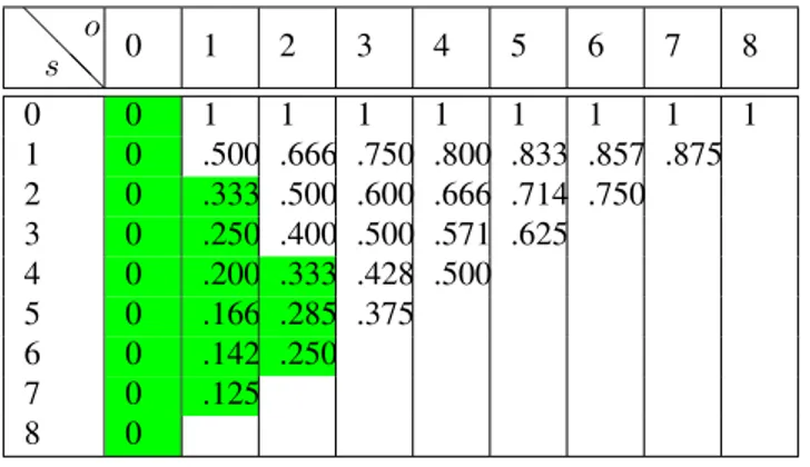
Table 1: Ratio between the number of neighbours of oppo-site type to the social degree: Qi=

oi

oi+si

Coloured values: agent ai, will be satisfied if Qiis under the

tolerancethreshold0.37 @ @_@ s o 0 1 2 3 4 5 6 7 8 0 0 1 1 1 1 1 1 1 1 1 0 .500 .666 .750 .800 .833 .857 .875 2 0 .333 .500 .600 .666 .714 .750 3 0 .250 .400 .500 .571 .625 4 0 .200 .333 .428 .500 5 0 .166 .285 .375 6 0 .142 .250 7 0 .125 8 0

In this model, all the agents have the same threshold of tolerance: it is a constant value (noted tolerance) which is fixed before the run. So, at each time t, for each agent ai,

equation 1 becomes:

satisf iedi(t) = (Qi(t) ≤ tolerance) (6)

The agents are said tolerant if the tolerance is greater than 0.5 (0.5 ≤ tolerance) and intolerant otherwise. We use the Mooreneighbourhood commonly employed in agent-based models. So the neighbours of an agent are those living in the eight nearest cells surrounding him and the degree di

is a number between 0 and 8. For instance, if the toler-ance threshold is 0.37, one particular agent ai, at time t,

will be satisfied if Qi(t) is under this value; this happens in

the following eighteen cases: (oi = 0), (si = 2, oi = 1),

(si = 3, oi = 1), (si = 4, oi = 1), (si = 5, oi = 1),

(si = 6, oi = 1), (si = 7, oi = 1), (si = 4, oi = 2),

(si= 5, oi = 2) and (si= 6, oi = 2) (see the coloured

val-ues on table 1). More, if there are exactly eight neighbours, i.e. di = 8, (see table 1, the diagonal line) such a tolerance

means that the agents are intolerant and cannot suffer more than two opposite neighbours.

How do unsatisfied agents move away ? In standard Schelling’s models agents move only to satisfy their own interest. This requires that agents must be able to access dis-tant information in order to determine whether or not it will be satisfied in a new vacant cell. This kind of behaviour is characteristic among economical agents that seek to maxi-mize their gain. Nonetheless such a behaviour come out of the idea of agents acting approximately rational, rather eco-nomically rational in terms of utility and breaks down the principle of locality(see Brownlee (2007)).

Global behaviour Regarding the micro-macro problem-atic, the Schelling model provides examples for the two

cases: [i → S] and [¯i → S] where i (resp. ¯i) stands for individual intolerance (resp. tolerance) and S stands for a high degree of global segregation. While the first case is the intuitive situation where micro-intolerance induces macro-segregation, the second case is more surprising as it shows that tolerant behaviours can nonetheless induce a global seg-regation.

The Schelling Model with the Eulogy to

Fleeing rule

In standard Schelling’s models agents aspire to satisfy their interests in the new places they move in. In this section, we rather assume a reaction from agent without real cognitive abilities expressed by the simple Eulogy to Fleeing rule (EF rule).

The Eulogy to Fleeing rule

The Eulogy to Fleeing rule is agreeing with the definition of the term satisficing proposed by Herbert A. Simon Simon (1956). ”Satisficing describes the selection of a good enough solution, the selection of a decision that meets a minimum threshold or aspiration level, the selection of which occurs in the context of incomplete information or limited compu-tation” Brownlee (2007).

The EF rule is defined as follows: for each unsatisfied agent, a cell is randomly chosen ’all over the world’ and the agent moves to this cell if and only if it is vacant. So the agents may move at random towards a new location ac-cording to their preferences by allowing utility-increasing or utility-decreasing actions. Moves do generate new satisfied or unsatisfied agents by a chain reaction until an equilibrium is reached. At a time t, if all the agents are satisfied, the EF rule has no effect and then such a configuration is a fixed pointfor the dynamics.

This simple rule is more in the spirit of the complex sys-tem paradigm, and, as locally there is no seeking for im-mediate benefits, it is interesting to know its global conse-quences. Although it is easy to build some particular cases where the EF rule does not converge, in the following sim-ulations this rule leads the system towards an equilibrium. Let’s note that although similar rules based on a random choice of vacant locations are already proposed (Edmonds and Hales (2005), Izquierdo et al. (2009)), they do not look completely identical to the EF rule. In particular, with the EF rule, an unsatisfied agent may stay in place for a while if the randomly chosen locations are occupied.

Simulation and results

In this paper, all the simulations are realized in the Net-Logo1 _{multiagent programmable modeling environment}

Pham (2004), Wilensky (1999). For each simulation, the agent’s features are updated in an asynchronous way and

1

the global geographic parameters are fixed. The world is a square of locations horizontally and vertically wrapped. An agent with type ’yellow’ (resp. green) is represented by a yellow (resp. green) square. A black square represents a va-cant location. A simulation stops at convergence, when all the agents become satisfied.

The world is a grid-square composed of10000 locations. This size is a good compromise between the necessity to have a large value to avoid small space effects and the con-venience to have a small value to achieve short computation time. There are1000 vacant locations, knowing that the den-sity rateis90% and 4500 agents in each type. We imposed a random initial configuration: in the cases studied below, the value of srandis indistinguishable from0.5; thus initial

configuration induces an aggregateIndex closed to0. We conducted two types of experiment: in the first one, all the agents are intolerant and in the second they are tolerant.

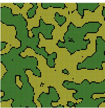
Intolerant agents For this first experiment the tolerance is set to0.37 (see table 1); so all the agents are intolerant. We can see in figure 1 the result of the agents spatio-temporal evolution at the end of a representative run: after1150 steps all the agents are satisfied (i.e. satisf actionRatio = 1), the mean Qiover the whole population (noted Q) is0.024

and the aggregateIndex is 0.957. From 100 indepen-dent runs we obtain, a mean of 0.952 (0.0041)2 _{for the}

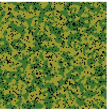
aggregateIndex and 0.024 (0.0022) respectively for Q. We can observe the emergence of large spatial homogeneous patterns. Moreover the borderland between the patterns is almost build with every vacant location (black square). So patterns are isolated by a no-man’s-land of vacant cells. Tolerant agents Here, the goal is to show that segrega-tion occurs even if no agent strictly prefers this. We set the toleranceto0.63 (see table 1), so all the individuals are tol-erant. In particular, if an agent has exactly eight neighbours, it can bear up to five opposite agents in its vicinity. Figure 2 gives an example of the evolution of the agents’ locations during a representative run. At the end, after 228 steps, all the agents are satisfied, the mean Qi over the whole

pop-ulation is0.229 and the aggregateIndex is 0.548. From 100 independent runs we obtain, a mean of 0.53 (0.0119) for the aggregateIndex and0.233 (0.0094) respectively for Q. While spatial segregation is not an attribute of the rational individuals’s behaviour, we can observe the emergence of many segregationist patterns, although they have a smaller size that in the previous case (see figure 1). More, vacant locations are scarce on borderline because with a high toler-ance level vacant cells are not requisite to delimit segrega-tionist patterns.

2

standard deviation is shown in ()

Figure 1: The Eulogy of Fleeing rule: tolerance= 0.37 View at convergence (ticks= 1150): Q = 0.024

aggregateIndex= 0.957

Discussion

In this section, we have shown that in spite of the use of a more simple and realistic local rule, the model produces a comparable global behaviour than the classical Schelling model.

We have shown that both intolerant and tolerant local be-haviours lead to the satisfaction of all the agents with the emergence of global segregationist patterns. Moreover, the gap between the tolerance and the mean Qiover the whole

population is surprisingly large at the end of a run. In this way complex dynamics build much more liveable configu-rations than necessary. With intolerant agents, vacant places are required to form the frontiers and insulate agents in ho-mogeneous patterns. In the next section, we propose to modify the model in order to insulate segregationist patterns without using vacant locations mainly.

From no-man’s-land to mediator-land

Most often, in real life some individuals are tolerant whereas others are intolerant. In a model, there are two ways to take into account this fact: either fixing a distribution for the tolerance, or dynamically evolving tolerance to ’converge’ toward a particular distribution. The first solution requires not only to choose one distribution: uniform, normal, pois-son,. . . but also to fix its parameters: mean and standard de-viation.

Figure 2: The Eulogy of Fleeing rule: tolerance= 0.63 View at convergence (ticks= 228): Q = 0.229

aggregateIndex= 0.548

Adaptive local rule

As we have no a priori on a target level of tolerance, we choose to start from an intolerant configuration and to ap-ply a local rule to gradually increase the tolerance. For in-stance, when a person is immersed in an unknown world, his first attempt will be to meet people which look like him; so initially, certainly with many apriority, such a person is gregarious or intolerant. Then, if his requirement is too high relatively to the environment, it will be difficult for him to find a fitting place; therefore a natural tendency will be to gradually reduce his stress by decreasing his gregariousness and/or increasing his tolerance.

In this new instance of the GMS, each agent has its own tolerance threshold. Furthermore, each individual threshold may vary over time. So, for each agent ai, at each time t,

the satisfied indicator (see equation 1) becomes:

satisf iedi(t) = (Qi(t) ≤ tolerancei(t)) (7)

Initially, the tolerance of each agent is set to a very small value, therefore an agent is at first radically intolerant and so will be unsatisfied. At each time, for each unsatisfied agent, a cell is randomly chosen ’all over the world’ in order to move in if it is vacant, otherwise, i.e. if the cell is already occupied, the agent stays put and adapts its own tolerance to the context by increasing its value with a small increment.

Simulation and results

For each agent, the tolerance is initialised to0.001 and we chose a small increment of0.003. We can see on figure 3 the spatio-temporal evolution of the agents at the end of a rep-resentative run. After663 steps all the agents are satisfied; the mean tolerance over the population is0.365, the mean Qi over the population is 0.049 and the aggregateIndex

is 0.892. Even if dynamics are more complex than in Schelling’s model, we can observe the emergence of spa-tial homogeneous patterns yet. On 100 runs we obtain, a mean of0.919 (0.0120) for the aggregateIndex and 0.360 (0.0047) respectively for the mean tolerance. So, on aver-age, dynamics lead agents to remain intolerant and a high segregation emerges at the global level; once again this is an example for the case[i → S].

Figure 3: Dynamic tolerance View at convergence (ticks= 663): aggregateIndex= 0.892 mean tolerance = 0.365 We can observe that the frontier between homogeneous patterns is constituted both by vacant cells (black square) and by the most tolerant agents (white circle), i.e. agents with tolerance ≥ 0.39; therefore, for a significant part, homogeneous regions are isolated by places for mediation where opposite agents may co-exist. We can note that there are also tolerant agents outside the mediator-land; this corre-sponds to scoria3_{in some areas where former conflicts have}

led to the local hegemony of one of the two types; thus data collected from the own tolerance of the agents allow to learn

3

Scoria is the dross that remains after the smelting of metal from an ore

more about the past of the system.

Discussion

A first result is that dynamics leads the mean tolerance to-ward a relatively weak value (0.36); as a consequence, when all the agents become satisfied, they remain on average in-tolerant. The second result is that segregation is still high (0.919). The third result is that in a world where agents are on average intolerant there are some tolerant agents which play a crucial role in the spatial distribution. This can serve as a clue to extend the model toward more mosaic-like struc-ture. Type-mix would be favoured by the existence of se-cluded agents amidst individuals having an opposite type. In the present model, this is impossible because agents are not tolerant enough to endure such a situation: we have to en-hance the dynamics to allow tolerance to reach high values. On the contrary, the presence of scoria shows that one agent with high tolerance may be useful in a moment at a place then becomes superfluous later in the same location; so de-crease the tolerance of satisfied agents may help to avoid such ’frozen region’. All this suggest us to manage two an-tagonist dynamics: increasing and decreasing the tolerance; so, we expect to significantly lower the level of segregation while maintaining a weak mean tolerance.

How to avoid high segregation ?

In this last section the goal is to respond to the question: How intolerant agents can become satisfied without the emergence of macro segregation?

In the new model we propose, there are two antagonist dynamics, the first one increases the tolerance of unsatisfied agents, whereas the second decreases the tolerance of satis-fied agents. Initially, the agents have a weak tolerance and are thus radically intolerant and unsatisfied.

• An unsatisfied agent, can either move to a vacant place or else simply increase its tolerance (for details, see the previous section).

• Conversely, for a satisfied agent ai, if the difference delta

between its toleranceiand the value of Qiin the place it

lives in is too high, its tolerance decreases.

In real life, when a person is no longer confronted with dis-tressing circumstance, his ability to cope later in such a sit-uation is reduced. This phenomenon can be explained by a mechanism of forgetfulness. In the model, an agent is satis-fied if it is not faced to a large enough number of opposite agents. If over time such a lack of confrontation persists, then the agent gradually reduces his threshold of tolerance.

Parameter space exploration

There are two main parameters that control the dynamics of tolerance: the amount of increment inc and decrement dec.

First we conduct a parameter space exploration in order to chose suitable values for the simulation.

In the context of complex systems, most often there are several parameters which together determine the global dy-namics. In order to choose values for the parameters used in the simulations, we have first conducted an exploration of the parameter space. The objective to minimize both the mean tolerance and the global aggregateIndex is difficult because when the first one decreases, the second increases and conversely. Therefore, we conduct a tradeoff-analysis to identify compromise for which the two criteria are mutually satisfied in a Pareto-optimal sense. This is a typical multi-objective optimisation problem where the optimal solutions correspond to a set of compromises expresses by a Pareto frontDyer et al. (1992), Belton and Stewart (2002). In prac-tice, the Pareto front is proposed to a human decision-maker who then chooses a solution according to his expertise.

For all the tests we perform, the parameter delta is set to 0.1. We focus our effort on areas that lead to interesting re-gions where convergence occurs with low tolerance and low segregation: each test corresponds to one couple(inc, dec) in the range[0.025, 0.040] × [0, 0.030]. There are 60 tests and, for each one, results are averaged over100 runs. Each data point of the scatter plot (see figure 4) corresponds to a couple(inc, dec) and represents both the aggregateIndex (y-value) and the mean tolerance (x-value) obtained when all the agents are satisfied. We can observe that heightening the parameter dec (while inc remains constant) pushes the point solution to the left toward the Pareto front. Conversely, lowering the parameter inc (while dec is constant) moves up the point solution on one front. This analysis leads us to choose a particular point on the Pareto-front that represents a good compromise between both intolerance and low seg-regation. To conduct the following simulations, we choose the point corresponding to the parameter values inc= 0.029 and dec= 0.017 (See the arrow on figure 4).

Results

Initially, all the tolerances are set to 0.1. We can ob-serve on figure 5 the spatial configuration at the end of a representative run when all the agents are satisfied: af-ter 513 steps, the mean Qi over the population is 0.306,

the mean tolerance over the population is 0.369 and the aggregateIndex is 0.383. On 100 runs, we obtain on average an aggregateIndex of 0.388 (0.0110) and a mean tolerance of 0.370 (0.0048). The value for the aggregateIndex (0.388) has to be compared with the ones obtained with the two previous models (0.957 and 0.919)

The frontier between homogeneous patterns is constituted by the most tolerant agents and there is no scoria inside the patterns. One observes that homogeneous areas are infil-trated by many secluded individuals: there are some niches which co-exist within a cohort of unlike agents; this is pos-sible only because loners are very tolerant. In contrast with

Figure 4: Parameter space analysis Tolerance vs. Segregation

the previous models, vacant locations don’t play any role in isolating individuals from each other. The most impor-tant feature of this model is that it prevents intolerant agents from high segregation. As the Schelling’s model provided an example for the case[¯i → S], this model exemplify the [i → ¯S] micro-macro link.

Conclusion and future work

In this article, we have proposed to extend the Schelling’s model considering that every individual has its own toler-ance level. In a first step we have proposed a simple way to locally manage the tolerance; all that gives rise to the emergence of a new kind of border and inner scoria both made up of the most tolerant agents. In a second stage, we have introduced new dynamics that consists of combining two antagonist strengths. As a result of this confrontation, the agents are able to reach an equilibrium where they all are satisfied, rather intolerant, but where the aggregation level remains low. As, at our knowledge, there is no prior work on this topic, this result is a significant challenge to the anal-ysis conducted by Schelling: it shows that one can avoid segregation if the tolerance level is adaptive, which is in our opinion a better assumption.

In future work, we will revisit those results by consid-ering situations closer to reality. Beyond a simple world of agents embedded on an homogeneous toroidal-grid, we have to consider different types of network as for example neigh-bourhoods defined from a scale-free network. We have ob-served the emergence of very different type of frontiers: no-man’s-land, mediator-land or in some extend mixing; thus,

Figure 5: Intolerant agents avoid global segregation View at convergence (ticks= 513): mean tolerance= 0.369, aggregateIndex = 0.383

it might be interesting to study for a border, its composition, its spatial distribution, its volume, porosity, permeability,... and so to better understand its function: place of exchange and/or medium to isolate.

Acknowledgements

We thank the referees for useful comments on the manuscript and Touria Ailt Elhadj for her english correction.

References

Banos, A. (2009). Exploring network effects in schelling? segre-gation model. S4-MODUS workshop Multi-scale interactions between urban forms and processes.

Belton, V. and Stewart, T. (2002). Multiple Criteria Decision Anal-ysis: An Integrated Approach. Springer-Verlag.

Brownlee, J. (2007). Satisficing, optimization, and adaptive sys-tems. CIS Technical Report 070305A.

Carrington, W. and Troske, K. (1997). On measuring segregation in samples with small units. Journal of Business & Economic Statistics, pages 402–409.

Dyer, J., Fishburn, P., Steuer, R., Wallenius, J., and Zionts, S. (1992). Multiple criteria decision making, multiattribute utility theory the next ten years. Management Science, 38(5):645–654.

Edmonds, B. and Hales, D. (2005). Computational simulation as theoretical experiment. Journal of Mathematical Sociology, 29(3):209–232.

Gerhold, S., Glebsky, L., Schneider, C., Weiss, H., and Zimmer-mann, B. (2008). Computing the complexity for schelling segregation models. Nonlinear Science and Numerical Simu-lation, 13 (10):2236–2245.

Goffette-Nagot, F., Jensen, P., and Grauwin, S. (2009). Dy-namic models of residential segregation: Brief review, analyt-ical resolution and study of the introduction of coordination. HAL-CCSD.

Izquierdo, L., Izquierdo, S., and Galan, J.and Santos, J. (2009). Techniques to understand computer simulations: Markov chain analysis. Journal of Artificial Societies and Social Sim-ulation, 12(16).

Pancs, R. and Vriend, N. (2003). Schelling’s spatial proximity model of segregation revisited. Computing in Economics and Finances.

Pham, D. (2004). From Agent-Based Computational Economics towards Cognitive Economics. in Bourgine P., Nadal J.P eds: Cognitive Economics: An Interdisciplinary Approach. Springer verlag.

Rosser, J. B. J. (1999). On the complexities of complex economics dynamics. Journal Of Economic Perspectives, 13:169–192. Schelling, T. C. (1971). Dynamic models of segregation. Journal

of Mathematical Sociology, 1:143–186.

Simon, H. A. (1956). Rational choice and the structure of the en-vironment. Psychological Review, 63:129–138.

Wilensky, U. (1999). Center for connected learning and computer-based modeling. http://ccl.northwestern.edu/netlogo/. Zhang, J. (2004). A dynamic model of residential segregation.