Device- and application-adapted quantum error correction

(1)

Device- and Application-Adapted Quantum Error

Correction

by

David Layden

B.S. Mathematical Physics, University of Waterloo (2014)

MMath Applied Mathematics, University of Waterloo (2016)

Submitted to the Department of Nuclear Science and Engineering

in partial fulfillment of the requirements for the degree of

Doctor of Philosophy in Quantum Science and Engineering

at the

MASSACHUSETTS INSTITUTE OF TECHNOLOGY

May 2020

c

○ Massachusetts Institute of Technology 2020. All rights reserved.

Author . . . .

Department of Nuclear Science and Engineering

May 20, 2020

Certified by. . . .

Paola Cappellaro

Professor of Nuclear Science and Engineering

Thesis Supervisor

Certified by. . . .

William D. Oliver

Associate Professor of Electrical Engineering and Computer Science

Thesis Reader

Accepted by . . . .

Ju Li

Battelle Energy Alliance Professor of Nuclear Science and Engineering

Professor of Materials Science and Engineering

Chair, Department Committee on Graduate Students

(2)

(3)

Device- and Application-Adapted Quantum Error Correction

by

David Layden

Submitted to the Department of Nuclear Science and Engineering on May 20, 2020, in partial fulfillment of the

requirements for the degree of

Doctor of Philosophy in Quantum Science and Engineering

Abstract

Precise control of coherent quantum systems could enable new generations of sensing, communication and computing technologies. Such systems, however, are typically noisy and difficult to stabilize. One promising technique to this end is called quantum error correction, which encodes quantum states in such a way that errors can be detected and corrected, much like in classical error-correcting codes.

Quantum error-correcting codes usually cast a wide net, in that they are designed to correct errors regardless of their physical origins. In large-scale devices, this is an essential feature. It comes at a cost, however: conventional quantum codes are typically resource-intensive in terms of both the system size and the control operations they require. Yet, in smaller-scale devices the main error sources are often well-understood. In the near term, it may therefore be advantageous to cast a more targeted net through specialized codes.

This thesis presents new families of such quantum error-correcting codes, which are adapted either for leading candidate devices, or for near-term applications. The device-adapted codes require exponentially less overhead than conventional codes to achieve the same level of protection, whereas the application-adapted codes can enhance quantum sensors, in which conventional codes cannot readily be used.

The new techniques presented in this thesis adapt cornerstones of conventional theory in light of key experimental challenges and opportunities. The ultimate goal of this research is to help bridge the gap between the exacting requirements of proposed quantum technologies and the realities of emerging quantum devices. Bridging this gap is critical, if quantum technologies are to realize their full potential.

Thesis Supervisor: Paola Cappellaro

(4)

(5)

Acknowledgments

This thesis is the culmination of a long process with many critical junctures. It is humbling to think of how strongly this process was shaped by the people surrounding me. Their contributions—big and small—compounded and intertwined so thoroughly that this end result would be inconceivable without them. I would therefore like to express my gratitude to a number of people while also stressing that this list is necessarily incomplete, both in breadth and in depth.

First, I wish to thank my supervisor Paola Cappellaro. The careful balance of freedom and guidance she offered, as well as her tireless support for her students (often behind the scenes), were essential to the success of this undertaking. I can only aspire to match her remarkable ability to see the forest through the trees, and to move seamlessly between fields in response to evolving problems. Working with her these past four years has been a privilege, and has shaped my approach to science and engineering.

I am also grateful to Liang Jiang, Seth Lloyd and Will Oliver for their guidance throughout my time at MIT. Liang’s ability to instantly isolate the core of a research problem, and Seth’s ability to spot such problems long before the rest of us come around, have been inspiring. Will’s technical expertise speaks for itself; I only hope I can be as kind and generous to those starting out as he is, should I ever find myself in his shoes.

I also wish to acknowledge my fellow Quantum Engineering Group members, past and present: Scott Alsid, Louisa Huang, J-C Jaskula, Changhao Li, Yixiang Liu, Dominika Lyzwa, Pai Peng, Akira Sone, Calvin Sun, Ken Wei, and Yuan Zhu for good times and useful discussions. Special thanks in particular to my friend and col-laborator Mo Chen, whose experimental know-how, unbounded network, and general joie de vivre have been a constant help.

Many thanks are also due to members of the MIT community and beyond, in-cluding Victor Albert, Ike Chuang, Eddie Farhi, Aram Harrow, Wolfgang Ketterle, Iman and Milad Marvian, Florentin Reiter, Peter Shor and Sisi Zhou, who have all

(6)

impacted my work in one way or another. The same goes for Brandy Baker, Heather Barry, Pete Brenton, and Dianne Lior, without whom things would presumably have derailed long ago. On a personal level, I am grateful to Jochen Braumüller, Peter Johnson and the Zapatistas, Bharath Kannan, and Morten Kjærgaard, with whom I’ve tackled many of life’s great questions while running along the Charles. Thank you also to Steve Girvin, Adrian Lupaşcu, Eduardo Martín-Martínez, and Michael Van-ner for fruitful discussions and hospitality over these last few years, and to Michael Goldberg, Sally Gunz, Kris Prather and Alex Vitkin for helping me figure out where I was going and how to get there. Thank you finally to Achim Kempf (a diplomat in a former life, surely) for his unwavering support. Things would look quite different were it not for him.

Lastly, none of this would have been possible without the immeasurable help of my parents, Richard and Ruth. I am eternally grateful to them. Thank you also to my mother-in-law Linda, for enabling the juggling act of the last few years, and for everything else. Finally, I don’t know where I would be without my wife. Sarah: thank you for making it all worthwhile.

(7)

List of Figures

1-1 Example of a quantum circuit . . . 24

1-2 Parity measurement . . . 28

1-3 Illustration of the Knill-Laflamme condition . . . 30

1-4 Bit-flip code circuit . . . 35

2-1 Performance comparison of QEC codes for normal 𝜃 . . . 58

2-2 Toy model encoding circuit . . . 59

2-3 Toy model recovery circuit . . . 60

2-4 2-qubit code encoding circuit . . . 62

2-5 2-qubit code recovery circuit . . . 62

2-6 Performance comparison of QEC codes for uniform 𝜃 . . . 65

2-7 2-qubit code pseudothresholds . . . 70

2-8 3-qubit code pseudothresholds . . . 70

2-9 Robustness of 2-qubit code pseudothresholds to transverse coupling . 73 2-10 Robustness of QEC code performance to model uncertainty vs. noise strength . . . 75

2-11 Robustness of QEC code performance to model uncertainty vs. number of qubits . . . 76

2-12 Scaling of QEC code robustness to model uncertainty . . . 76

3-1 Fidelity for different feedback strategies . . . 87

3-2 Feedback strategy phase diagram . . . 88

(12)

5-1 QEC for sensing: negative noise correlations . . . 129

5-2 QEC for sensing: positive noise correlations . . . 136

5-3 QEC for sensing: robustness . . . 138

5-4 QEC codes for sensing on 𝑛 = 3 qubits . . . 142

6-1 Ring of sensing qubits illustration . . . 167

A-1 Validation of Monte Carlo averaging for strong noise . . . 178

A-2 Validation of Monte Carlo averaging for weak noise . . . 179

(13)

Citations to Previously Published

Work

Most chapters of this thesis are based on material which has appeared in print else-where. By chapter number:

Chapter 2 D. Layden, M. Chen, P. Cappellaro, Phys. Rev. Lett. 124, 020504 (2020). c

○ 2020 American Physical Society.

Chapter 3 D. Layden, L. R. Huang, P. Cappellaro, to appear in Quantum Sci. Technol. (2020).

Chapter 5 D. Layden, P. Cappellaro, npj Quantum Inf. 4, 30 (2018).

Chapter 6 D. Layden, S. Zhou (equal contributions), P. Cappellaro, L. Jiang, Phys. Rev. Lett. 122, 040502 (2019). c○ 2019 American Physical Society.

(14)

(15)

Preface

“After growing wildly for years, the field . . . appears to be reaching its infancy.” – John R. Pierce Quantum mechanics has been revolutionized in recent decades by two comple-mentary advances. The first advance is theoretical: a number of protocols have been proposed wherein a coherent quantum system, through careful control, could be made to output useful information that a classical system of equivalent size could not pro-duce. Among these protocols are quantum algorithms with dramatically better scal-ing than their known classical counterparts on a number of important computational problems, as well as schemes for measuring physical quantities with unprecedented sensitivity and resolution. Other related protocols enable encrypted communication whose security relies on the laws of quantum physics rather than on computational complexity.

The second advance is experimental. The phenomena of quantum superposi-tion and entanglement, which underlie the protocols above, were largely confined to gedanken experiments for much of the 20th _{century. As a result of steady,}

interdisci-plinary progress, however, researchers can now create, control, and measure coherent quantum systems of appreciable size with impressive precision. There are several different types of such quantum systems, based on superconducting circuits, trapped ions, neutral atoms, nuclear and electronic spins, and photons, to name a few, as well as combinations thereof. To some extent, these different platforms are equivalent; for instance, the same quantum algorithm run on any two of them should produce the same output, regardless of the underlying device and its physics. This has allowed

(16)

the two aforementioned advances to occur largely in parallel, requiring relatively little close interaction between the communities responsible for each.

As we progress along the path towards implementing these protocols and realiz-ing true quantum-coherent technologies (henceforth simply “quantum technologies”), however, a new paradigm is emerging. It is not yet clear on which types of devices these technologies will ultimately rely; yet, some of the physics and engineering chal-lenges with which they will likely contend have become apparent. These include the dominant error mechanisms in leading candidate systems, as well as challenges inherent in specific applications, such as quantum sensing. Incorporating these exper-imental concerns directly into theory—using a level of abstraction somewhere between those typical in the theoretical and experimental communities—is a promising way to shorten the path towards useful quantum technologies.

This device- and application-adapted approach is timely, as many quantum de-vices are entering a gray area wherein they are neither obviously useful, nor obviously useless. That is, they are too small and too noisy for most proposed protocols, and yet, they are increasingly hard to mimic classically. For instance, a fledgling quantum computer recently outperformed a supercomputer on an ad hoc problem (with few clear applications) [1]. Theory closely informed by experiment can provide a power-ful means for getting the most out of these limited—yet increasingly substantive— devices. Therefore, barring an unexpected hardware breakthrough, it will likely be a critical ingredient in moving from proof-of-principle demonstrations to useful early applications in the coming years.

An important area where this approach could have a substantial impact is in noise suppression, and in quantum error correction (QEC) more specifically. As mentioned above, noise sets an important—if not the main—limit on current quantum devices. Not only are quantum systems often highly susceptible to small disturbances, but their manifestly quantum nature prohibits straightforward feedback stabilization, as this would collapse their state. QEC encompasses a family of noise-suppression tech-niques which use encoding and (typically) feedback based on partial measurements to stabilize quantum systems without completely collapsing their states. In effect, it is

(17)

a method of making a noisy quantum device behave like a smaller, but less noisy one; that is, of trading off size for reduced noise. It is a remarkably powerful tool, which conventionally requires little physical knowledge of the noise afflicting a device. In fact, this feature underpins QEC’s envisioned role as the main tool to reduce noise to tolerable levels for large-scale quantum technologies. Characterizing the noise mecha-nisms in a quantum device can be exponentially hard in the device size; conventional QEC casts a wide enough net to avoid this eventual bottleneck.

Of course, casting such a wide net comes at a price: conventional QEC is very resource-intensive. Stated differently, it trades device size for reduced noise at a rate too exacting to be useful in most current and emerging devices [2]. This thesis in-stead takes a more targeted approach to QEC, which is directly informed by current experiments. Part I deals with device-adapted QEC, and shows that one can dramat-ically improve QEC’s efficiency in leading candidate devices by incorporating their underlying physics from the start. Part II focuses on the specific QEC challenges posed by quantum sensing, rather than on a particular physical device, and devel-ops application-adapted QEC schemes where conventional ones do not work. Taken together, both parts aim to help bridge the gap between the long-term plans for han-dling noise in large quantum devices, and the reality of current experiments. This is a critical task, if the long-term plans for quantum technologies are to be realized at all.

(18)

Part I

Device-Adapted Quantum Error

Correction

(19)

Chapter 1 Introduction

1.1 Formalism

This thesis deals exclusively with finite-dimensional quantum systems; that is, those with a finitely many energy eigenstates. These ubiquitous systems underlie many current candidate realizations of quantum technologies. Their states are most simply represented by a vector |𝜓⟩ in a complex vector space H = C𝑑 _{(𝑑 < ∞), called the}

system’s Hilbert space. Since most envisioned quantum technologies involve many interacting subsystems, we will often be concerned with the aggregate Hilbert space arising from those of various subsystems. If subsystems 1 and 2 have Hilbert spaces H1 and H2 of dimensions 𝑑1 and 𝑑2 respectively, their combined Hilbert space is the

tensor product of H1 and H2, written H = H1 ⊗ H2, of dimension 𝑑 = 𝑑1𝑑2. For

our purposes, states in H1⊗ H2 and matrices on it can be constructed in any basis

by using as a definition 𝐴⊗ 𝐵 = ⎛ ⎜ ⎜ ⎜ ⎝ 𝑎11𝐵 · · · 𝑎1𝑛𝐵 ... ... ... 𝑎𝑚1𝐵 · · · 𝑎𝑚𝑛𝐵 ⎞ ⎟ ⎟ ⎟ ⎠ , (1.1)

for arbitrary matrices/vectors 𝐴 = (𝑎𝑖𝑗) (taken here to be 𝑚 by 𝑛) and 𝐵. For

(20)

state |𝜓1⟩ ⊗ |𝜓2⟩ ∈ H , often written as |𝜓1⟩ |𝜓2⟩ or |𝜓1𝜓2⟩, can be constructed using

Eq. (1.1). We will largely be concerned with two-level systems, whose basis states are often denoted as |0⟩ and |1⟩ ∈ C2_{. As such systems are the quantum analogs}

of classical bits of information, they are often called qubits (pronounced “Q-bits”). The aggregate Hilbert space for 𝑛 qubits is H = C2𝑛

, a convenient basis for which is the set of states corresponding to classical 𝑛-bit strings, e.g., |010 . . . 0⟩. This is often called the computational basis. Note that not all states in C2𝑛

can be factored into an 𝑛-fold tensor product; those that can are said to be separable, and those that cannot are said to be entangled. The latter are distinctly non-classical, and form a key ingredient for most quantum technologies.

Calculating quantum measurement outcomes in this description often involves taking inner products—here, simply the dot product on C𝑑_{. It is useful to define}

the dual space H* _{to H , comprising the set of linear maps ⟨𝜓| from H to C. H}*

is also a vector space, and it has the same structure as H (more precisely, they are isomorphic). In fact, if |𝜓⟩ is written out as a 𝑑-dimensional column vector, ⟨𝜓| is simply the corresponding row vector with each element replaced by its complex conjugate. In this notation, the inner product between |𝜓⟩ and |𝜑⟩ is simply ⟨𝜓|𝜑⟩. For |𝜓⟩ to encode a valid quantum state, we will demand that it have unit length, i.e., that ⟨𝜓|𝜓⟩ = 1. Moreover, states which represent mutually-exclusive classical outcomes, such as computational basis states, are taken to be orthogonal.

Quantum measurements are described by a set of linear operators (for 𝑑 < ∞, simply matrices) {𝑀𝑗}, where 𝑀𝑗 encodes the 𝑗th potential measurement outcome.

The probability of getting this outcome for a system in state |𝜓⟩ is

𝑝𝑗 =⟨𝜓| 𝑀𝑗†𝑀𝑗|𝜓⟩ = ||𝑀𝑗|𝜓⟩ ||2, (1.2)

where 𝑀†

𝑗 is called the adjoint of 𝑀𝑗and denotes its conjugate transpose, and || |𝑥⟩ || =

√︀⟨𝑥|𝑥⟩. To ensure that these probabilities sum to unity for all |𝜓⟩, the measurement operators must satisfy ∑︀_𝑗𝑀_𝑗†𝑀𝑗 = 𝐼. If a measurement returns the 𝑗th outcome, the

(21)

𝑝𝑗 = 0the corresponding post-measurement state is irrelevant). Physically, this means

that measurements are typically destructive in quantum mechanics. For instance, the most common measurements involve 𝑀𝑗 =|𝑗⟩⟨𝑗| for some orthogonal basis of states

{|𝑗⟩}. Before the measurement, the system’s state can be a general superposition of these |𝑗⟩’s, i.e., |𝜓⟩ = ∑︀𝑗𝑐𝑗|𝑗⟩, but interaction with the measurement device causes

the system to collapse to a particular state |𝑗⟩ with probability 𝑝𝑗 = |𝑐𝑗|2. This

collapse makes straightforward feedback stabilization impossible; if a generic state |𝜓⟩ has been subject to an unknown disturbance, there is no general way to measure the impact on the system and correct accordingly without collapse.

The dynamics of a closed quantum system is described by the Schrödinger equa-tion:

𝑖~𝑑

𝑑𝑡 |𝜓(𝑡)⟩ = 𝐻(𝑡) |𝜓(𝑡)⟩ , (1.3)

where 𝐻(𝑡) is the system’s Hamiltonian, the matrix encoding its energy levels. This dynamics can equivalently be written as |𝜓(𝑡)⟩ = 𝑈(𝑡) |𝜓(0)⟩, where the matrix-valued function 𝑈(𝑡) satisfies the same differential equation as |𝜓(𝑡)⟩:

𝑖~𝑑

𝑑𝑡𝑈 (𝑡) = 𝐻(𝑡)𝑈 (𝑡). (1.4)

To simplify the notation, we will often leave the time dependence implicit in this and similar equations. Moreover, throughout this thesis we will use units in which ~ = 1, unless otherwise stated. Since 𝐻 is Hermitian/self-adjoint (𝐻 = 𝐻†_{), 𝑈 is unitary}

(𝑈†_{= 𝑈}−1_{). This ensures that 𝑈 preserves the length of state vectors, and therefore}

represents a valid evolution.

The Hamiltonian of a single qubit can always be written as a real linear combina-tion of 𝐼 (the identity matrix) and the “Pauli matrices”

(22)

which have the form 𝑋 = ⎛ ⎝ 0 1 1 0 ⎞ ⎠ 𝑌 = ⎛ ⎝ 0 −𝑖 𝑖 0 ⎞ ⎠ 𝑍 = ⎛ ⎝ 1 0 0 ₋₁ ⎞ ⎠ (1.6)

in the computational basis. These matrices are sometimes denoted as 𝜎𝑥, 𝜎𝑦 and

𝜎𝑧, although in this thesis our notation will prove more convenient. The reason

𝐼, 𝑋, 𝑌 and 𝑍 span all possible qubit Hamiltonians is that they form a basis for matrices on C2_{. More precisely, any 2 × 2 Hermitian matrix can be expressed as}

as a linear combination of 𝐼, 𝑋, 𝑌 and 𝑍 with real coefficients, and any general 2 × 2 matrix can be expressed as a complex combination thereof. Furthermore, Pauli matrices have a natural geometric interpretation: the eigenstates of 𝑋, 𝑌 , and 𝑍 encode the possible outcomes of measuring a spin-1

2 system in the spatial 𝑥, 𝑦, and 𝑧

directions respectively. More generally, a generic Hamiltonian for 𝑛 non-interacting qubits (which does not produce entanglement) is in span{𝐼, 𝑋𝑗, 𝑌𝑗, 𝑍𝑗}, where for

instance

𝑋3 = 𝐼 ⊗ 𝐼 ⊗ 𝑋 ⊗ 𝐼 ⊗ · · · ⊗ 𝐼

⏟ ⏞

𝑛−3

(1.7) acts as 𝑋 on qubit 3 and trivially on the others. A key property of tensor products is

(𝐴_{⊗ 𝐵)(𝐶 ⊗ 𝐷) = (𝐴𝐶) ⊗ (𝐵𝐷),} (1.8)

for matrices/vectors 𝐴, 𝐵, 𝐶 and 𝐷 of compatible sizes. This means that we can write more general Hamiltonians describing coupled subsystems (which produce en-tanglement) compactly, e.g.:

𝐻 = 𝜔1 2 𝑍⊗ 𝐼 + 𝜔2 2 𝐼⊗ 𝑍 + 𝐽𝑋 ⊗ 𝑋 = 𝜔1 2 𝑍1+ 𝜔2 2 𝑍2+ 𝐽𝑋1𝑋2. (1.9) Note that it is common to drop certain 𝐼’s and ⊗ symbols to simplify the notation, when such shorthand introduces no ambiguity.

(23)

𝐻 = 𝐻0+𝐻1 has well-understood part 𝐻0, and a part 𝐻1to be analyzed more closely,

one can absorb the effects of 𝐻0 into the frame of reference, therefore isolating those

of 𝐻1. More precisely, a state |𝜓⟩ in the “lab frame” becomes 𝑒𝑖𝐻0𝑡|𝜓⟩ in this rotating

frame. One can easily show that this rotating frame state satisfies the Schrödinger equation, but with 𝐻 replaced by ˜𝐻1(𝑡) = 𝑒𝑖𝐻0𝑡𝐻1𝑒−𝑖𝐻0𝑡. Similarly, an operator 𝑀 in

the lab frame, such as a measurement operator, becomes ˜𝑀 (𝑡) = 𝑒𝑖𝐻0𝑡_{𝑀 𝑒}−𝑖𝐻0𝑡 in the rotating frame. When [𝐻0, 𝑀 ] := 𝐻0𝑀−𝑀𝐻0 = 0, however, 𝑀 is not affected by the

change of frame; a common reason for choosing 𝐻0to commute with the measurement

operators one plans to implement. Note that we have implicitly assumed 𝐻0 to be

time-independent here. This is not strictly necessary, although it is the relevant case for this thesis.

It is often convenient to coarse-grain quantum dynamics into lumped unitaries 𝑈, describing a system’s net evolution over some time interval, and thus abstracting away the fine-grained description of how this evolution occurred. This is an efficient way to describe quantum control sequences and algorithms; one can specify a desired sequence of lumped operations (often in a rotating frame) whose effect is readily understood, which can then be translated into a more opaque time-dependent Hamil-tonian to be implemented. Common examples of such 𝑈’s acting on single qubits are Pauli matrices (which are both unitary and Hermitian) and Hadamard matrices:

𝐻 = √1 2 ⎛ ⎝ 1 1 1 −1 ⎞ ⎠. (1.10)

Unfortunately Hadamard matrices and Hamiltonians share the same symbol; however, the intended meaning of 𝐻 is usually clear from context. Another important type of lumped 𝑈 is that of controlled operations, which act on a qubit (called the target) only if another (called the control) is in the state |1⟩. One common example is the controlled-𝑍 or controlled-phase operation, denoted 𝑐𝑍, which acts as

(24)

qubit 1 |0⟩ 𝐻

qubit 2 |0⟩ 𝑍

qubit 3 |1⟩ 𝐻

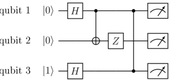
Figure 1-1: An example of a quantum circuit, showing three qubits initially prepared in the state |001⟩, which are then subject to: (i) 𝐻 ⊗𝐼 ⊗𝐻 where 𝐻 is the Hadamard operation, (ii) a 𝑐NOT with qubits 1 and 2 as the control and target respectively, (iii) 𝑍2, and (iv) a controlled-𝑍, whose action is symmetric under the exchange of control

and target qubits, which are therefore denoted with the same symbol. Finally, the qubits are measured in the computational basis, producing various 3-bit strings with known probabilities. The circuits in this thesis were made using Ref. [3].

where the first qubit is the control and the second is the target. Note that since both qubits may start in superposition states, this is an entangling operation that can produce non-classical effects; in particular, it can modify the control qubit’s state. A closely related operation is the controlled-𝑋 or controlled-NOT, whose name derives from the fact that the Pauli 𝑋 acts like a NOT gate in classical logic. It has the effect

𝑐NOT = |0⟩⟨0| ⊗ 𝐼 + |1⟩⟨1| ⊗ 𝑋. (1.12)

It is often useful to represent these and other operations using circuit diagrams, inspired by classical logic circuits, as illustrated in Fig. 1-1. These circuits can be used to represent quantum control sequences (at a high level) and algorithms.

The framework introduced so far is that of pure states, which have zero entropy. We now introduce the more general formalism of density matrices, which can describe both pure and mixed states, the latter having non-zero entropy. This thesis will use both formalisms; while that of density matrices is more powerful in principle, that of pure states provides an easier means of understanding aspects of quantum error correction. To motivate the definition of density matrices, we note that the dynamics of a quantum system may not be identical in every run of an experiment, e.g., due to random variations in the system’s environment. For instance, rather than

(25)

evolving each time by the same unitary 𝑈, a system may evolve by different 𝑈(𝜃)’s, each occurring with probability 𝑝(𝜃). One might expect the average dynamics to be described by ∫︀ 𝑝(𝜃)𝑈(𝜃)𝑑𝜃, but upon substituting this into Eq. (1.2), one sees that it does not give the correct averaged probabilities of measurement outcomes.

A more general description of a quantum state, which can encompass such uncer-tainty, is as a density matrix 𝜌 = 𝜌†_{with tr(𝜌) = 1 and with non-negative eigenvalues.}

In this description, a state vector |𝜓⟩ becomes 𝜌 = |𝜓⟩⟨𝜓|. If a density matrix 𝜌 can be written as |𝜓⟩⟨𝜓| (i.e., if it has a rank of 1), it is said to represent pure state; otherwise, it represents a mixed state with nonzero entropy. Any mixed state can be expressed as a probabilistic mixture of orthogonal pure states, 𝜌 = ∑︀𝑗𝜆𝑗|𝜓𝑗⟩⟨𝜓𝑗|, where the

𝜆𝑗’s can be interpreted as probabilities. It is this decomposition that will allow us

to move smoothly between the density matrix and state vector formalisms. For den-sity matrices, Eq. (1.2) becomes instead 𝑝𝑗 = tr(𝑀𝑗†𝑀𝑗𝜌), and the post-measurement

state for outcome 𝑗 is given by 𝑀𝑗𝜌𝑀𝑗†/𝑝𝑗 (provided again 𝑝𝑗 ̸= 0; when 𝑝𝑗 = 0 the

corresponding post-measurement state is irrelevant). Notice that an average of den-sity matrices (e.g., over noise realizations) gives the correct averaged measurement probabilities, as desired. Moreover, if a quantum system becomes entangled with its environment, the system’s effective (mixed) state can always be expressed as a density matrix.

In the language of density matrices, the Schrödinger equation takes the form 𝑑𝜌

𝑑𝑡 =−𝑖[𝐻, 𝜌], (1.13)

which is sometimes called the quantum Liouville equation. It can be written more compactly by introducing the notion of a superoperator: a linear function on the space of matrices, which in turn act on H . In effect, a superoperator is to a density matrix 𝜌 what a matrix is to a state vector |𝜓⟩. In particular, defining the Hamiltonian superoperator ℋ by its action on a density matrix as ℋ(𝜌) := [𝐻, 𝜌], Eq. (1.13) takes the simple form of ˙𝜌 = −𝑖ℋ(𝜌). Just as a unitary matrix 𝑈 encoded the evolution of a state vector under the Schrödinger equation, the same evolution of a density

(26)

matrix is described by the superoperator 𝒰, defined as 𝒰(𝜌) := 𝑈𝜌𝑈†_{, which can be}

found by integrating the quantum Liouville equation (or equivalently, the Schrödinger equation).

The Schrödinger and quantum Liouville equations describe unitary dynamics (so called because 𝑈† _{= 𝑈}−1_{). Such dynamics underpins most proposals for quantum}

technologies. In experiments, however, dynamics are seldom exactly unitary. Instead, they typically also have an irreversible character, in which information encoded in a quantum state is gradually lost, due to growing entanglement with an environment or classical noise processes affecting the system’s Hamiltonian. We will refer to such imperfect systems as being open. The gradual loss of information in open quantum systems is broadly called decoherence, and it is arguably the central obstacle to developing useful quantum technologies. The aim of quantum error correction is to effectively suppress decoherence, so as to make real open quantum systems behave almost like ideal closed ones, in effect.

In principle it is possible to write an equation of motion for any open quantum system, analogous to the Schrödinger/quantum Liouville equations for closed systems [4, 5]. In practice this is rarely useful for two reasons: First, one often has little knowledge of the environment’s internal dynamics, nor the exact nature of its coupling to the system. Second, even if one had this knowledge, the system’s resulting equation of motion would almost surely be too complex to solve. Instead, one is typically forced to use a more empirically-motivated, effective description of open system dynamics in order to make progress. This can be as much an art as it is a science; there are many ways to model open quantum systems, and a model well-suited for one system and purpose can fail to capture important details of others.

Just as we can coarse-grain unitary quantum dynamics into a lumped matrix 𝑈, we can encode the net effect of both unitary and non-unitary quantum dynamics into a superoperator 𝒦 called a quantum channel (under the reasonable assumption that the system was not initially correlated with its environment), whose name derives from classical information theory. Whereas 𝑈 must be unitary to describe a valid closed quantum dynamics, 𝒦 must be completely positive and trace-preserving (CPTP, as

(27)

well as Hermiticity preserving). For our purposes, it suffices to say that any 𝒦 admits a “Kraus decomposition,” that is, it can be written as a sum

𝒦(𝜌) = ∑︁

𝑗

𝐾𝑗𝜌𝐾𝑗†, (1.14)

where {𝐾𝑗} are matrices known as Kraus operators of 𝒦, which have the property that

∑︀

𝑗𝐾𝑗†𝐾𝑗 = 𝐼. This expression generalizes the unitary superoperator 𝒰 encoding the

dynamics of the Schrödinger/Liouville equations, which has a single Kraus operator 𝑈. It is important to note that Kraus decompositions are not unique in general; rather, the same generic quantum channel 𝒦 could be written in terms of different Kraus operators {𝐾′

𝑗} ̸= {𝐾𝑗}. In fact, quantum channels generally admit infinitely

many Kraus decompositions, and we are free to pick the most convenient one—a fact that is important for quantum error correction.

1.2 Quantum Error Correction

The ubiquity of decoherence, together with the destructive nature of quantum mea-surements, would seem to prohibit the building of useful, controllable large-scale quantum devices. Mathematically, this difficulty is reflected in part by the fact that most quantum channels 𝒦 describing non-unitary dynamics do not have an inverse channel. That is, there is generally no physically realizable 𝒦−1_{—even in principle—}

such that 𝒦−1_{𝒦 = ℐ, where ℐ denotes the identity channel (i.e., ℐ(𝜌) = 𝜌 for all}

𝜌). More broadly, there is generally no channel 𝒢 such that 𝒢𝒦 represents a unitary evolution.

Thankfully, there is a loophole which could allow decoherence to be effectively suppressed through quantum error correction (QEC). It relies on two key observations: First, we don’t necessarily need to reverse decoherence on all quantum states; instead, we could realize quantum technologies by doing so only on a subset of them. Second, measurement need not completely collapse a quantum state. Rather than measuring whether a system is in some particular state |𝑗⟩, one can instead measure whether it

(28)

|𝜓⟩ |0⟩

Figure 1-2: A parity measurement performed indirectly on the top two qubits, which realizes the measurement operators 𝑀0 = |00⟩⟨00| + |11⟩⟨11| and 𝑀1 =

|01⟩⟨01| + |10⟩⟨10|. For an initial state |𝜓⟩ = 𝑐00|00⟩ + 𝑐01|01⟩ + 𝑐10|10⟩ + 𝑐11|11⟩,

the measurement returns 0 with probability 𝑝0 = |𝑐00|2+|𝑐11|2, and returns 1 with

probability 𝑝1 = |𝑐01|2+|𝑐10|2. In either case, the state of the top two qubits is not

totally collapsed, but instead projected into the even or odd parity subspaces respec-tively (namely, onto span{|00⟩ , |11⟩} or span{|01⟩ , |10⟩}). In particular, these qubits remain entangled after the measurement for a generic |𝜓⟩.

is in some larger set of states. An example of such a measurement, which is usually performed indirectly with the help of an ancillary qubit (called an ancilla), is shown in Fig. 1-2.

To see how QEC exploits these observations, we will start with an abstract picture, and then gradually build up a more concrete description until we can finally meld in the physics of certain quantum devices. QEC makes use of states within a special subspace C0 of H , called the codespace, over which 𝒦 can be reversed. (At least

approximately.) Typically, on a system of 𝑛 qubits the codespace has dimension dim(C0) = 2𝑘 for 𝑘 < 𝑛, meaning it has the same structure as (i.e., is isomorphic to)

the Hilbert space of a smaller, 𝑘-qubit system1_{. We can therefore define a basis of}

orthogonal codeword states {|0 . . . 00l⟩ , |0 . . . 01l⟩ , . . . , |1 . . . 11l⟩} for C0, labeled by

𝑘-bit strings with a subscript l for “logical.” Ultimately, QEC will provide a method by which 𝑛 noisy qubits can be made to behave like 𝑘 less noisy ones, at the cost of an 𝑛− 𝑘 qubit overhead, as well as additional control operations. The 𝑘 effective qubits encoded in C0 ⊂ H are called logical qubits, in contrast to the 𝑛 physical qubits.

The idea is to prepare some initial logical state |𝜓l⟩ ∈ C0, and to perform

opera-tions and measurements on the 𝑛 physical qubits which effectively enact desired ones at the logical level, i.e., on the 𝑘 logical qubits. The typical QEC strategy is to

peri-1_{Of course, dim(H ) and dim(C}₀₎ _{need not be powers of 2—nor even finite—in general [6].}

However, we will focus on the qubit case here for concreteness, as it will be the most relevant for this thesis.

(29)

odically detect and correct errors from decoherence (and perhaps also from imperfect control and measurements) all the while. For this latter part to be possible, we must choose an appropriate codespace C0 for the channel 𝒦 representing the decoherence

we aim to reverse. Ideally, it should be chosen such that each of the Kraus operators 𝐾𝑗 of 𝒦 maps states in C0 to mutually orthogonal subspaces C𝑗 without distortion.

Let’s unpack this statement and make it more precise.

1.2.1 Knill-Laflamme Condition

Much like classical error correction, QEC requires one to identify “which error oc-curred” in a quantum system (or whether an error occurred at all), in the typical parlance. The meaning of this phrase will be explained shortly. Unlike in classi-cal error correction, however, in QEC one must take care to identify errors without destroying the encoded state. To see how this is possible, consider the action of a channel 𝒦 describing decoherence on an initial logical state 𝜌l =|𝜓l⟩⟨𝜓l|:

𝒦(𝜌l) = 𝐾1|𝜓l⟩⟨𝜓l| 𝐾1†+ 𝐾2|𝜓l⟩⟨𝜓l| 𝐾2†+ . . . . (1.15)

Suppose that each 𝐾𝑗 mapped a generic |𝜓l⟩ out of C0 and into some new subspace

C𝑗 (independent of |𝜓l⟩), and that all of these subspaces were mutually

orthogo-nal, as illustrated in Fig. 1-3a. Then, measuring which subspace the system was in would produce a pure post-measurement state 𝐾𝑗|𝜓l⟩⟨𝜓l| 𝐾𝑗†/𝑝𝑗—or, written as a

state vector, 𝐾𝑗|𝜓l⟩ /√𝑝𝑗 ∈ C𝑗—with probability 𝑝𝑗 = ⟨𝜓l| 𝐾𝑗†𝐾𝑗|𝜓l⟩. (If 𝑝𝑗 = 0

the corresponding post-measurement state is irrelevant and undefined.) Therefore, even though 𝒦 encompassed all of the Kraus operators {𝐾𝑗} at once, this choice of

codespace would allow us to only worry about correcting one at a time. In fact, it would allow us to think of the 𝐾𝑗’s as mutually-exclusive errors, each occurring with

some probability 𝑝𝑗; and of the measurement as revealing only the “error syndrome”

𝑗, telling us which error occurred without fully collapsing the system’s state.

Mathematically, to find such a codespace we demand that any two logical states |𝜓l⟩ and |𝜑l⟩ ∈ C0be mapped to different orthogonal subspaces C𝑗 and C𝑘by different

(30)

Hilbert space

codespace

error subspace

(a) Orthogonal subspaces

codespace error subspace

(b) No distortion

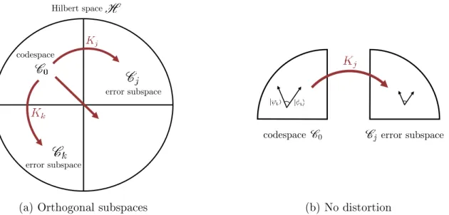
Figure 1-3: Our two requirements for QEC codes. Left: Distinct Kraus operators 𝐾𝑗

and 𝐾𝑘 (𝑗 ̸= 𝑘) must map all states in the codespace C0 into orthogonal subspaces

C𝑗 and C𝑘 respectively. Right: Each 𝐾𝑗 must preserve the angle between any two

logical states |𝜓l⟩ , |𝜑l⟩ ∈ C0 (or cause both to vanish).

errors 𝐾𝑗 and 𝐾𝑘:

⟨𝜓l| 𝐾𝑗†𝐾𝑘|𝜑l⟩ = 0 (𝑗 ̸= 𝑘), (1.16)

as in Fig. 1-3a. This will allow us to identify which error occurred through measure-ment. However, simply identifying an error is not enough to reverse its effect. For instance, knowing that a qubit emitted a photon and decayed to state |0⟩ does not enable one to restore its full initial state 𝛼 |0⟩+𝛽 |1⟩. Additionally, we must insist that 𝐾𝑗 not distort states as it maps them from C0 to C𝑗. For starters, this means that if

𝑝𝑗 = 0for some |𝜓l⟩ ∈ C0 (that is, if 𝐾𝑗|𝜓l⟩ = 0), 𝑝𝑗 must be identically zero for all

logical states. More broadly, when 𝑝𝑗 ̸= 0, we must demand that the angle between

arbitrary initial states and that between the corresponding post-measurement states be the same, as illustrated in Fig. 1-3b, that is:

⟨𝜓l|𝜑l⟩ = 1

||𝐾𝑗|𝜓l⟩ || ||𝐾𝑗|𝜑l⟩ ||⟨𝜓l| 𝐾 †

𝑗𝐾𝑗|𝜑l⟩ , (1.17)

for all |𝜓l⟩ , |𝜑l⟩ ∈ C0. This will allow us to correct the post-measurement states

(31)

invert-ible. In particular, if two logical states are orthogonal, their corresponding post-measurement states must be too. It follows immediately that 𝑝𝑗 must be independent

of the initial state. This was to be expected; were it not the case, the error syndrome measurement would reveal information about the encoded state, thus damaging it. In aggregate, our requirement that 𝐾𝑗 cause no distortion amounts to demanding

⟨𝜓l| 𝐾𝑗†𝐾𝑗|𝜑l⟩ = 𝜆𝑗⟨𝜓l|𝜑l⟩, (1.18)

for all |𝜓l⟩ , |𝜑l⟩ ∈ C0, where 𝜆𝑗 is some constant that depends only on 𝑗.

Combined, the two requirements derived above become

⟨𝜓l| 𝐾𝑗†𝐾𝑘|𝜑l⟩ = 𝜆𝑗𝛿𝑗𝑘⟨𝜓l|𝜑l⟩ for all |𝜓l⟩ , |𝜑l⟩ ∈ C0. (1.19)

We can re-write this expression in a more useful form by defining the orthogonal projector 𝑃 onto the codespace:

𝑃 =

2𝑘−1

∑︁

𝑖=0

|𝑖l⟩⟨𝑖l| , (1.20)

where |𝑖l⟩ denotes the binary representation of 𝑖 (for instance |2l⟩ = |0 . . . 010l⟩). In

terms of 𝑃 , Eq. (1.19) becomes simply

𝑃 𝐾_𝑗†𝐾𝑘𝑃 = 𝜆𝑗𝛿𝑗𝑘𝑃. (1.21)

One step remains. We mentioned in Section 1.1 that a quantum channel generically admits infinitely many Kraus decompositions. More precisely, if {𝐾𝑗} are Kraus

operators for 𝒦, then so too are {𝐾′ 𝑗 =

∑︀

𝑘𝑣𝑗𝑘𝐾𝑘} for any unitary matrix 𝑉 = (𝑣𝑗𝑘).

In this derivation we have implicitly chosen a convenient set of Kraus operators which highlighted the underlying structure of QEC. Of course, all Kraus decompositions for 𝒦 are physically equivalent, so our result should not depend on having chosen a particular one. Rather, in terms of the generic Kraus operators {𝐾′

(32)

equation becomes

𝑃 𝐾_𝑗′†𝐾_𝑘′𝑃 = 𝑚𝑗𝑘𝑃. (1.22)

where 𝑀 = (𝑚𝑗𝑘)is known as the code matrix, and has eigenvalues2spec(𝑀) = {𝜆𝑗}.

Eq. (1.22) is the famous Knill-Laflamme condition [7], which can equivalently be written as

𝑃 𝐾_𝑗′†𝐾𝑘′𝑃 ∝ 𝑃. (1.23)

While we have derived it as a sufficient condition for QEC, it is in fact both sufficient and necessary for the existence of a quantum channel that reverses 𝒦 over a subspace C0 ⊂ H [7]. To simplify the notation, we will henceforth drop the prime marks (′)

on the 𝐾′

𝑗’s, and use {𝐾𝑗} to denote a generic set of Kraus operators for the channel

𝒦.

As presented here, QEC looks very much like classical error correction, in the sense that both use clever encodings to identify and reverse discrete errors. However, the state space of 𝑛 qubits is much broader than that of 𝑛 classical bits. Quantum systems can therefore be affected by noise in a wide range of ways which have no classical analogs. Fortunately, QEC is a remarkably powerful tool for reversing such a contin-uum of decoherence processes. Specifically, a QEC code that can reverse some channel 𝒦 over a codespace C0 ⊂ H will do the same for any other channel ˜𝒦 ̸= 𝒦 whose

Kraus operators are linear combinations of 𝐾𝑗’s (not necessarily related through a

unitary). This follows immediately from the Knill-Laflamme condition. There is no reason to view the Kraus operators of 𝒦 as being more natural or fundamental to the code than those of ˜𝒦, even though they are not generally equivalent. This suggests that we ought not think of QEC as necessarily correcting a discrete set of physical errors, each of which afflicting the system with some probability per unit time, nor as being tied to any particular channel. Rather, we should think of it as casting a “net” which can catch a continuum of possible errors, and of this net’s precise shape as being specified through a list of discrete errors. More specifically, imagine designing

2_{Choosing different Kraus decompositions for 𝒦 amounts to expressing 𝑀 in different bases. Our}

(33)

a QEC code such that 𝑃 𝐸†

𝑗𝐸𝑘𝑃 ∝ 𝑃 for some desired set of “error operators” {𝐸𝑗},

which one is free to choose. Then, the effect of any matrix in E = span{𝐸𝑗}—the

continuous “net” cast by the code in this metaphor—on a logical state can be reversed. One has wide discretion in specifying these error operators {𝐸𝑗} when designing a

QEC code; for instance, they need not accurately describe the decoherence in a par-ticular device, so long as the true Kraus operators for this decoherence are contained in E . (Since we care only about the “net” E resulting from {𝐸𝑗}, we can equivalently

pick different error operators with the same span.) A central theme of this thesis, however, is that QEC codes designed around an E which closely reflects the actual decoherence mechanisms in a device—that is, casting a targeted net— can provide substantial benefits.

Example 1: Idealized Bit Flips

Consider for illustration 𝑛 = 3 qubits subject to the decoherence channel

𝒦(𝜌) = (1 − 3𝑝)𝜌 + 𝑝(𝑋1𝜌𝑋1 + 𝑋2𝜌𝑋2+ 𝑋3𝜌𝑋3); (1.24)

a highly idealized model in which a bit-flip error (|0⟩ ↔ |1⟩) occurs on at most one qubit with some probability 𝑝. While there is no inverse channel 𝒦−1_{, we can reverse}

𝒦 over a two-dimensional subspace, i.e., encode 𝑘 = 1 logical qubit in this system using the code C0 =span{|0l⟩ , |1l⟩}, where |0l⟩ = |000⟩ and |1l⟩ = |111⟩. The Kraus

operators 𝐾𝑗 = √𝑝𝑋𝑗 (for 1 ≤ 𝑗 ≤ 3) map states in the codespace to the error

subspaces

C1 =span{|100⟩ , |011⟩} C2 =span{|010⟩ , |101⟩} C3 =span{|001⟩ , |110⟩}

(34)

without distortion, and 𝐾0 = √1− 3𝑝 𝐼 acts trivially. That is, 𝑃 = |000⟩⟨000| +

|111⟩⟨111| satisfies the Knill-Laflamme condition as required, with a code matrix

𝑀 = ⎛ ⎜ ⎜ ⎜ ⎜ ⎜ ⎜ ⎝ 1− 3𝑝 0 0 0 0 𝑝 0 0 0 0 𝑝 0 0 0 0 𝑝 ⎞ ⎟ ⎟ ⎟ ⎟ ⎟ ⎟ ⎠ (1.26)

with respect to {𝐾𝑗}3𝑗=0. This code casts a net defined by the error operators {𝐸𝑗} =

{𝐼, 𝑋1, 𝑋2, 𝑋3}, whose span is E . In this first example, the Kraus operators 𝐾𝑗

describing the decoherence are simply proportional to these abstract error operators around which the code is designed. We will see in later examples how this need not be the case.

One can reverse the action of 𝒦 over C0 by majority vote. As we have argued,

however, it is imperative that the error detection process reveal only whether the state is in C0, C1, C2 or C3, but nothing about the encoded information. This can

be done by measuring the parity between each pair of qubits, as in Fig. 1-2, rather than measuring any individual qubit’s state. If each pair of qubits has even parity then no error occurred, and there is no need for feedback. Otherwise, one can infer which error occurred—or in this case, simply on which qubit it occurred—using the syndrome measurement outcomes for each of the three pairs, and by applying 𝑋 to the errant qubit. In fact, it is not necessary to measure the parity of all three qubit pairs; one gets the same information from measuring only two of them. The complete process of error detection and correction, which we will call the recovery, is shown in Fig. 1-4.

This code is called the bit-flip code. Notice that if the Kraus operators described phase-flip errors instead (𝐾𝑗 ∝ 𝑍𝑗, producing |1⟩ ↔ − |1⟩ on qubit 𝑗), one could

instead use |0l⟩ = |+++⟩ and |1l⟩ = |−−−⟩, where |±⟩ := √1₂(|0⟩ ± |1⟩) and 𝑍 |±⟩ =

|∓⟩. Errors could be detected by measuring parity in the |±⟩ basis, and corrected by applying 𝑍𝑗’s rather than 𝑋𝑗’s. This latter code is called the “phase flip code.”

(35)

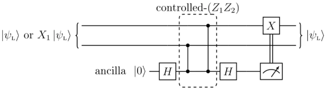
|𝜓⟩ 𝒦 𝑋𝑗 |𝜓⟩ |0⟩ |0⟩ |0⟩ |0⟩ |0⟩ 𝐻 𝐻 |0⟩ 𝐻 𝐻 controlled-(𝑍1𝑍2) controlled-(𝑍2𝑍3) recovery

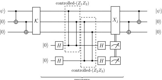
Figure 1-4: A circuit showing: (i) the encoding of a physical qubit into the bit-flip code, (ii) exposure to the channel 𝒦, (iii) a recovery consisting of two parity measurements followed by the application of 𝐼, 𝑋1, 𝑋2 or 𝑋3 as needed, and (iv) the

mapping of the encoded state back to the first physical qubit. Note that double wires denote the transmission of classical information, and that we have expressed the same parity measurements found in Fig. 1-2 in terms of Hadamard and c𝑍 operations, for reasons that will be explained in Section 1.2.4. Finally, in practice one may want to avoid converting between physical and logical states as shown here, and instead work only with encoded states at every step.

(36)

both simply called repetition codes, after the family of classical error-correcting codes which encode each bit into 𝑛 ≥ 3 copies (i.e., 0 ↦→ 0 . . . 0 and 1 ↦→ 1 . . . 1). Like their classical counterparts, these quantum error-correcting codes are the smallest instances in a family of codes. The 𝑛 = 3 repetition code can correct single 𝑋𝑗 errors (or linear

combinations of these) at the cost of an 𝑛 − 𝑘 = 2 qubit overhead. One can instead encode a logical qubit (𝑘 = 1) into 𝑛 = 5 physical qubits through |𝑖l⟩ = |𝑖𝑖𝑖𝑖𝑖⟩ for

𝑖 = 0/1 and correct for arbitrary bit flips on up to two qubits through a majority vote (similarly for the phase-flip code). This increased protection, which leads to a wider “net” E = span{𝐼, 𝑋𝑗, 𝑋𝑗𝑋𝑘} comes at the expense of an increased overhead of

𝑛_{− 𝑘 = 4. More generally, correcting for arbitrary bit or phase flips on ≤ 𝑤 qubits} with a repetition code requires an overhead of 𝑛 − 𝑘 = 2𝑤 qubits.

1.2.2 Role of Quantum Error-Correcting Codes

Notice that the circuit in Fig. 1-4 represents a multi-step procedure, whereas the Knill-Laflamme condition specifies only an abstract codespace C0 =range(𝑃 ). There

are two reasons why we will often treat such QEC codespaces as fundamental in this thesis, and focus on them accordingly. First, a QEC code satisfying the Knill-Laflamme condition automatically implies the form of an appropriate feedback cor-rection scheme. Second, a QEC code can also be used to implement open-loop error suppression.

Let us briefly expand on the first point. Suppose {𝐸𝑗} are error operators for a

QEC code that have been chosen to produce a diagonal code matrix, i.e., 𝑃 𝐸†

𝑗𝐸𝑘𝑃 =

𝛿𝑗𝑘𝜆𝑗𝑃. Such 𝐸𝑗’s exist for any appropriate E . For each nonzero 𝜆𝑗, one can define

a unitary 𝑈𝑗 by performing a polar decomposition of 𝐸𝑗𝑃 to give

𝐸𝑗𝑃 = √︀𝜆𝑗𝑈𝑗𝑃. (1.27)

We can then define orthogonal projectors 𝑃𝑗 := 𝑈𝑗𝑃 𝑈𝑗† onto the error subspaces

(37)

condition. Finally, it is straightforward to show that the channel ℛ(𝜌) := ∑︁

𝑗|𝜆𝑗̸=0

𝑈_𝑗†𝑃𝑗𝜌𝑃𝑗𝑈𝑗 (1.28)

reverses any channel 𝒦 with Kraus operators in E on a logical state 𝜌l:

ℛ[︀𝒦(𝜌l)]︀ = 𝜌l, (1.29)

Note that ℛ describes the process of measuring operators {𝑃𝑗}, then applying the

unitary 𝑈†

𝑗 in the event of outcome 𝑗. Therefore, as claimed above, a QEC code

C0 and a set of error operators {𝐸𝑗} together imply a closed-loop correction scheme

[7, 8].

Now the second point. Rather than correct errors explicitly, one could think of making them energetically unfavorable and thus unlikely to occur, instead of correct-ing them when they do [9]. This could be done by engineercorrect-ing a system Hamiltonian with low-energy eigenstates forming a desired error-correcting code3_{, separated from}

higher-energy states by a large energy gap. Such a Hamiltonian could be realized through strong, carefully designed couplings between qubits, for instance. The result would be a system with a low-energy subspace in which decoherence is exponentially suppressed in the size of the energy gap (under quite general assumptions about the environment) [10–12]. For instance, a register of qubits with a Hamiltonian

𝐻 = 1 2 ∑︁ 𝑗 𝜔𝑗𝑍𝑗− ∑︁ 𝑗𝑘 𝐽𝑗𝑘𝑍𝑗𝑍𝑘, (1.30)

with sufficiently strong couplings 𝐽𝑗𝑘 > 0will have a protected subspace corresponding

to the bit-flip code. We will not deal explicitly with such open-loop error suppression techniques in this thesis. However, it is natural to think of some of the results presented here in this context. Since both the closed- and open-loop control schemes discussed above are ultimately specified by a codespace C0 ⊂ H , we will often treat

3_{In fact, an error-detecting code, which reveals when an error occurs though not necessarily which}

(38)

the latter as the core of QEC. Example 2: Local Phase Flips

Let us build up towards more realistic decoherence models by considering the single-qubit channel

𝒦1(𝜌) = (1− 𝑝)𝜌 + 𝑝𝑍𝜌𝑍, (1.31)

representing a phase error with probability 𝑝. The aggregate channel4 _{for 𝑛 qubits}

undergoing 𝒦1 simultaneously (and independently) is denoted 𝒦⊗𝑛1 =𝒦1⊗ · · · ⊗ 𝒦1.

Notice that for 𝑛 = 3 this is not the same (contrived) channel as in Example 1 with 𝑋 ↔ 𝑍. Here we do not artificially impose that errors can occur only on one qubit at once; rather, since each qubit is subject to an independent decoherence process, errors can occur on 𝑤 qubits with probability 𝑂(𝑝𝑤₎_{. For 𝑛 = 3, 𝒦}⊗𝑛

1 has Kraus operators 𝐾0 = (1− 𝑝)3/2𝐼 𝐾1 =√𝑝(1− 𝑝)𝑍1 𝐾2 =√𝑝(1− 𝑝)𝑍2 𝐾3 =√𝑝(1− 𝑝)𝑍3 𝐾4 = 𝑝√︀1 − 𝑝𝑍1𝑍2 𝐾5 = 𝑝√︀1 − 𝑝𝑍2𝑍3 𝐾6 = 𝑝√︀1 − 𝑝𝑍1𝑍3 𝐾7 = 𝑝3/2𝑍1𝑍2𝑍3, (1.32)

describing errors on 0 to 3 qubits by descending rows. We can still use the repeti-tion code (this time for phase-flips) to suppress the decoherence described by this channel; however, we cannot hope to reverse it exactly, even over the codespace, as the number of Kraus operators grows too fast with 𝑛. This follows from a simple counting argument: 𝒦⊗𝑛

1 has 2𝑛 distinct Kraus operators in general. To have one

perfect logical qubit, we would need to decompose the total Hilbert space H into 2𝑛 _{orthogonal 2-dimensional subspaces}5 _C

0,C1, . . . ,C2𝑛₋₁. Since dim(H ) = 2𝑛, this is clearly impossible. Instead, we must make due with reversing the most damaging

4_{In general a density matrix for a bipartite system can be decomposed into a linear combination}

of separable matrices 𝜌𝑖⊗ 𝜌𝑗. The overall action of subsystem superoperators 𝒜 and ℬ, described by

the joint superoperator 𝒜⊗ℬ can be understood through its action (𝒜⊗ℬ)(𝜌𝑖⊗𝜌𝑗) =𝒜(𝜌𝑖)⊗ℬ(𝜌𝑗). 5_{Unless one can find a “degenerate code,” in which distinct Kraus operators act identically on}

(39)

Kraus operators; here, those of largest magnitude. Note that this means the error “net” E can no longer simply coincide with span{𝐾𝑗}7𝑗=0; this example therefore begins

to illustrate the distinction between the Kraus operators of a physical decoherence process {𝐾𝑗}, and the more abstract error operators {𝐸𝑗} = {𝐼, 𝑍1, 𝑍2, 𝑍3} around

which the code is built.

For 𝑛 = 3, the effect of 𝒦⊗𝑛

1 followed by a recovery using the repetition code is

𝜌l ↦→ ℛ[︀𝒦⊗31 (𝜌l)]︀ = (1 − 𝑝eff)𝜌 + 𝑝eff𝑋l𝜌𝑋l, (1.33)

where 𝑝eff = 𝑝2(3− 2𝑝) is smaller than the physical error probability 𝑝 when 𝑝 < 1/2,

and 𝑋l maps |0l⟩ ↔ |1l⟩. That is, at the logical level, the system behaves not like a

noiseless qubit, but like a less noisy one, provided the physical noise strength is below a threshold value. While {𝐾𝑗}𝑗≥1 can be viewed as describing physical errors, 𝑋l

describes a “logical error” occurring with probability 𝑝eff. For 𝑛 = 3 𝑝eff = 𝑂(𝑝2), and

more generally 𝑝eff = 𝑂(𝑝

𝑛+1

2 ) with these codes, reflecting the fundamental trade-off of QEC: decreased space for reduced noise.

Example 2 illustrates a common reality. A channel describing the open dynamics of a real quantum device is generally too complex (i.e., has too many Kraus oper-ators, with too complicated a time dependence) to be exactly reversed over some codespace—even in principle. In this sense, all QEC is approximate QEC in practice. We will therefore aim to get the best logical error rates using the fewest possible resources in this thesis, by targeting the dominant decoherence mechanisms inherent in specific devices and applications.

1.2.3 Lindblad Equation

Moving closer yet to a picture of QEC in real devices, we introduce a simple model for the dynamics of open quantum systems called the Lindblad equation [13]:

𝑑𝜌 𝑑𝑡 =−𝑖[𝐻, 𝜌] + ∑︁ 𝑗𝑘≥1 𝑑𝑗𝑘 (︁ 𝐴𝑗𝜌𝐴†_𝑘− 1 2{𝐴 † 𝑘𝐴𝑗, 𝜌} )︁ . (1.34)

(40)

Here 𝐻 is the system’s Hamiltonian, 𝐷 = (𝑑𝑗𝑘)is a positive semidefinite matrix (i.e.,

Hermitian with non-negative eigenvalues), {𝐴𝑗} are arbitrary matrices on H , and

{𝐴, 𝐵} := 𝐴𝐵 + 𝐵𝐴 is an anti-commutator. There are numerous ways to derive the Lindblad equation. For instance, by postulating that the quantum channel which propagates a system from time 𝑡 to 𝑡 + 𝛿𝑡 depend only on 𝛿𝑡, one arrives at Eq. (1.34) from the channel’s Kraus decomposition in the 𝛿𝑡 → 0 limit. More physically, one can arrive at the same equation by considering a system weakly coupled to an environment in which information about the system dissipates quickly compared to the system dynamics of interest [14, 15]. In Part II we will arrive at Eq. (1.34) differently still by analyzing the effect of a classical noise process on a quantum sensor. Suffice it to say that the Lindblad equation is an important tool for modeling open quantum systems. It therefore behooves us to connect it with the QEC formalism introduced thus far.

Eq. (1.34) can be written compactly as 𝑑𝜌

𝑑𝑡 =−𝑖ℋ(𝜌) + 𝒟(𝜌) (1.35)

in terms of the Hamiltonian superoperator ℋ(𝜌) := [𝐻, 𝜌] and the “dissipator” 𝒟(𝜌) = ∑︁ 𝑗𝑘≥1 𝑑𝑗𝑘 (︁ 𝐴𝑗𝜌𝐴†𝑘− 1 2{𝐴 † 𝑘𝐴𝑗, 𝜌} )︁ . (1.36)

One can go a step further and define the superoperator ℒ = −𝑖ℋ + 𝒟, often called the Lindbladian superoperator, which has both Hamiltonian and dissipative parts, ℋ and 𝒟 respectively. The Lindblad equation then becomes ˙𝜌 = ℒ(𝜌). If 𝒟 = 0, the Lindblad equation reduces to the quantum Liouville equation for a closed system. As the name would suggest, however, a vanishing 𝒟 generally introduces a non-unitary, irreversible character to the dynamics.

Notice that the sum in Eq. (1.34) runs over 𝑗 and 𝑘. It is an important fact that one can always get rid of the 𝑗 ̸= 𝑘 cross-terms in this sum by expressing 𝒟 in terms of new operators. Concretely, let 𝑊 be a unitary matrix which diagonalizes 𝐷:

(41)

where {𝛾𝑗} are the eigenvalues of 𝐷. Such a 𝑊 is guaranteed to exist. Then, one can re-write 𝒟 as 𝒟(𝜌) =∑︁ 𝑗≥1 (︁ 𝐿𝑗𝜌𝐿†𝑗− 1 2{𝐿 † 𝑗𝐿𝑗, 𝜌} )︁ , (1.38)

in terms of the “jump operators”

𝐿𝑗 = √𝛾𝑗

∑︁

𝑘≥1

𝑤𝑘𝑗𝐴𝑗. (1.39)

These are so named because one can interpret each 𝐿𝑗𝜌𝐿†𝑗 term in 𝒟 as describing

the occurrence of a discrete jump/error 𝐿𝑗 on the system with some probability per

unit time, determined by 𝛾𝑗, within an otherwise-unitary dynamics [16, 17]. (The

−1 2{𝐿

†

𝑗𝐿𝑗, 𝜌} terms ensure proper normalization when no such jump occurs.)

This “diagonal” (i.e., having no cross-terms) form of 𝒟 allows us to straightfor-wardly understand QEC in the language of Lindblad dynamics. To do so, consider the channel 𝒦 describing Lindblad evolution for some short time 𝑡, which is given for-mally by 𝒦 = 𝑒ℒ𝑡 _{(assuming ℒ is time-independent, otherwise the expression should}

include a time-ordered integral). In general, Kraus operators of 𝒦 will depend on 𝑡 in complicated ways. However, we can expand them in powers of 𝑡 and solve for the leading-order parts quite easily. Consider some initial state 𝜌 evolving under Eq. (1.34) for a short time 𝑡. To first order in the evolution time 𝑡 the state becomes 𝒦(𝜌) = 𝜌 + 𝑡 [︂ (︁ − 𝑖𝐻 − 1₂∑︁ 𝑗≥1 𝐿†_𝑗𝐿𝑗 )︁ 𝜌 + 𝜌(︁_{− 𝑖𝐻 −}1 2 ∑︁ 𝑗≥1 𝐿†_𝑗𝐿𝑗 )︁† +∑︁ 𝑗≥1 𝐿𝑗𝜌𝐿†𝑗 ]︂ ⏟ ⏞ ℒ(𝜌) +𝑂(𝑡2₎ = 𝐾0𝜌𝐾0†+ ∑︁ 𝑗≥1 𝐾𝑗𝜌𝐾𝑗†+ 𝑂(𝑡 2 ), (1.40) where 𝐾0 = 𝐼− 𝑡 (︁ 𝑖𝐻 + 1 2 ∑︁ 𝑗≥1 𝐿†_𝑗𝐿𝑗 )︁ + 𝑂(𝑡2) and 𝐾𝑗≥1 = √ 𝑡𝐿𝑗+ 𝑂(𝑡3/2). (1.41)

(42)

get time-averaged operators in the expressions above.) Because Kraus operators always act on 𝜌 from both sides as 𝐾𝑗𝜌𝐾𝑗†, expanding 𝒦 = 𝑒ℒ𝑡 = ℐ + ℒ𝑡 + . . . in

powers of 𝑡 produces Kraus operators in integer powers of √𝑡. We cannot generally hope to correct 𝒦 to all orders in 𝑡, just as we could not do so for all powers of 𝑝 in Example 2. As in that example though, we can aim to correct the most damaging errors perturbatively, to order 𝑂(𝑡). This amounts to demanding that

𝑃 𝐾₀†𝐾𝑗𝑃 ∝ 𝑃 + 𝑂(𝑡3/2), (1.42)

𝑃 𝐾_𝑗†𝐾𝑘𝑃 ∝ 𝑃 + 𝑂(𝑡3/2), (1.43)

and

𝑃 𝐾₀†𝐾0𝑃 ∝ 𝑃 + 𝑂(𝑡3/2), (1.44)

for all 𝑗, 𝑘 ≥ 1. In terms of operators appearing in the Lindblad equation, these requirements are equivalent to

𝑃 𝐿𝑗𝑃 ∝ 𝑃, (1.45)

𝑃 𝐿†_𝑗𝐿𝑘𝑃 ∝ 𝑃, (1.46)

and

𝑃 𝐻𝑃 _{∝ 𝑃,} (1.47)

respectively [18, 19]. This means that to suppress the dissipative part of a Lindblad dynamics to leading order in time, one should use a code for which {𝐼, 𝐿𝑗} ⊂ E .

If one also wants to suppress the Hamiltonian part of the dynamics through QEC, one also needs 𝐻 ∈ E . (This may or may not be desirable, and can also be done e.g., through dynamical decoupling, as we will see in Part II.) The idea is to perform QEC recoveries frequently as compared to the relevant timescale set by {𝐿𝑗} and/or

𝐻 (often in a rotating frame), so as to keep uncorrected 𝑂(𝑡2₎ _{terms from becoming}

important. One could also use a code which corrects to higher orders in 𝑡 through a broader E , thus further reducing—though never completely nullifying—the logical error rate.

(43)

Example 3.1: Independent Dephasing

Consider for illustration the purely dissipative Lindblad equation 𝑑𝜌 𝑑𝑡 = 1 2𝑇* 2 3 ∑︁ 𝑗=1 (︁ 𝑍𝑗𝜌𝑍𝑗− 𝜌 )︁ (1.48) on 𝑛 = 3 qubits. One can easily show that the resulting dynamics coincides with the channel 𝒦⊗3

1 from Example 2, with 𝑝 = (1−𝑒−𝑡/𝑇

*

2)/2. The 3-qubit repetition code can therefore largely suppress this decoherence when recoveries are repeated frequently compared to the dephasing time 𝑇*

2. Over longer timescales, however, higher-order

errors start to become significant, causing substantial decoherence at the logical level.

Example 3.2: Independent Dephasing with a Hamiltonian

Suppose there is also a Hamiltonian component to the above dynamics, namely: 𝑑𝜌 𝑑𝑡 =−𝑖[𝐻, 𝜌] + 1 2𝑇* 2 3 ∑︁ 𝑗=1 (︁ 𝑍𝑗𝜌𝑍𝑗 − 𝜌 )︁ . (1.49) for 𝐻 = 1

2(𝜔1𝑍1+ 𝜔2𝑍2+ 𝜔3𝑍3). An initial logical state of the repetition code 𝜌l that

is corrected after a time 𝑡 will become

𝜌_l _{↦→ ℛ(𝑒}ℒ𝑡𝜌_l) = 𝜌_l+ 𝑂(𝑡2_), _(1.50)

regardless of the exact values of 𝜔𝑗 and 1/𝑇2*, provided all are sufficiently small

com-pared to 𝑡−1 _{for this perturbative expansion to be meaningful. This insensitivity of}

the code to the precise dynamics is because the Kraus operators of 𝑒ℒ𝑡_{, truncated}

to order 𝑂(𝑡), are contained in the code’s error “net” E = span{𝐼, 𝑍1, 𝑍2, 𝑍3}. Note

however, that these short-time Kraus operators are now not equal to—nor propor-tional to—the error operators 𝐼, 𝑍1, 𝑍2, and 𝑍3; they only have the same span. This

(44)

Example 3.3: Correlated Dephasing with a Hamiltonian

Finally, consider the Lindblad equation 𝑑𝜌 𝑑𝑡 =−𝑖[𝐻, 𝜌] + 1 2𝑇* 2 3 ∑︁ 𝑗,𝑘=1 (︁ 𝑍𝑗𝜌𝑍𝑘− 1 2{𝑍𝑗𝑍𝑘, 𝜌} )︁ , (1.51) where 𝐻 = 𝜔 2(︀𝑍1+ 𝑍2+ 𝑍3). (1.52)

We will see how such dynamics can arise in Part II. Upon diagonalizing 𝒟, one finds that it has but a single non-vanishing jump operator, 𝐿1 ∝ 𝑍1 + 𝑍2 + 𝑍3 ∝ 𝐻. Of

course, the repetition code can still reverse this dynamics to leading order in time for logical states. Here, however, not only are 𝐻 and 𝐿1 not Pauli operators, they

(together with 𝐼) do not span E for this code. Rather, they span only a subset of E (namely, span{𝐼, 𝑍1 + 𝑍2 + 𝑍3}), suggesting that the repetition code might be

overkill here; i.e., that its error “net” is bigger than needed. This is indeed the case. Consider instead the following code on any two qubits: |0l⟩ = |01⟩ and |1l⟩ = |10⟩.

Not only does this code satisfy the Knill-Laflamme condition, it is a “decoherence-free subspace” (DFS) of this dynamics, meaning that there is no need to actually correct errors (i.e., ℛ = ℐ), since the codespace is immune to them from the start. Note that this code/DFS does not correct for single-qubit phase flips, by design. Rather, it uses our knowledge of the dynamics to cast a more targeted “net” ˜E , and achieves (in principle) a vanishing logical error rate while reducing the overhead by half. This example illustrates clearly the distinction between the error operators around which a code is designed and the physical Kraus operators to be corrected. Moreover, it shows that choosing error operators carefully in light of the decoherence at hand, and designing new QEC codes from these error operators, can be quite beneficial. We will expand broadly on this approach in later chapters.

(45)

1.2.4 Choosing Error Operators

Based on this last example, the reader may wonder why most of the codes we have considered so far were constructed using bit or phase flips as error operator. As-suming nature has no special affinity for Pauli matrices, why are they so central to these and many other QEC codes? It is not because they are the Kraus operators describing decoherence in all leading quantum devices. Rather, it is because they have convenient mathematical properties, which in turn, lead to QEC codes with nice features; notably, these codes require remarkably little knowledge of the deco-herence mechanisms against which they protect. This is a potentially critical feature for implementing QEC in large systems, where fully characterizing decoherence is all but impossible. Of course, this generality comes at a cost: the Pauli-centric approach to QEC can require prohibitive overheads in many devices, and can be largely in-compatible with near-term applications like quantum sensing. This would seem to severely limit the utility of these codes in existing and emerging quantum devices. In this thesis we will largely consider codes built around non-Pauli errors, designed specifically for such devices. Before getting into these, however, it is useful to establish a baseline by briefly discussing Pauli-based QEC codes.

Strong, many-body interactions are rare in quantum systems. This means we generically expect quantum devices to couple to their environments in a predomi-nantly local way; that is, through an interaction Hamiltonian that acts non-trivially on only one qubit (or perhaps few qubits) at a time, e.g.,

𝐻_int _≈∑︁ 𝑗 (︀𝐼 ⊗ · · · ⊗ 𝐼 ⊗ 𝐻𝑗 ⏟ ⏞ qubit 𝑗 ⊗𝐼 · · · ⊗ 𝐼)︀ ⊗ 𝐻𝐸𝑗 ⏟ ⏞ environment . (1.53)

Recall that {𝐼, 𝑋, 𝑌, 𝑍} is a basis for all Hermitian matrices on single qubits, of which 𝐻𝑗 is one. Similarly, any 2-qubit Hermitian matrix can be written as a linear

combi-nation of tensor products of 𝐼, 𝑋, 𝑌 and 𝑍, and so on for multi-qubit Hamiltonians. This means that, quite generally, a QEC code built around an error “net” E compris-ing all scompris-ingle-qubit Paulis can suppress the effects of local couplcompris-ing to an environment,

Device- and application-adapted quantum error correction

Device- and Application-Adapted Quantum Error

Correction

by

David Layden

B.S. Mathematical Physics, University of Waterloo (2014)

MMath Applied Mathematics, University of Waterloo (2016)

Submitted to the Department of Nuclear Science and Engineering

in partial fulfillment of the requirements for the degree of

Doctor of Philosophy in Quantum Science and Engineering

at the

MASSACHUSETTS INSTITUTE OF TECHNOLOGY

May 2020

c

○ Massachusetts Institute of Technology 2020. All rights reserved.

Author . . . .

Department of Nuclear Science and Engineering

May 20, 2020

Certified by. . . .

Paola Cappellaro

Professor of Nuclear Science and Engineering

Thesis Supervisor

Certified by. . . .

William D. Oliver

Associate Professor of Electrical Engineering and Computer Science

Thesis Reader

Accepted by . . . .

Ju Li

Battelle Energy Alliance Professor of Nuclear Science and Engineering

Professor of Materials Science and Engineering

Chair, Department Committee on Graduate Students

Device- and Application-Adapted Quantum Error Correction

by

David Layden

Abstract

Acknowledgments

Contents

I Device-Adapted Quantum Error Correction

18

II Application-Adapted Quantum Error Correction

92

Appendices

175

List of Figures

Citations to Previously Published

Work

Preface

Part I

Device-Adapted Quantum Error

Correction

Chapter 1

Introduction

1.1 Formalism

1.2 Quantum Error Correction

1.2.1 Knill-Laflamme Condition

1.2.2 Role of Quantum Error-Correcting Codes

1.2.3 Lindblad Equation

1.2.4 Choosing Error Operators