Nuclear forces at the extremes

(1)

HAL Id: tel-02082089

https://tel.archives-ouvertes.fr/tel-02082089

Submitted on 28 Mar 2019

HAL is a multi-disciplinary open access archive for the deposit and dissemination of sci-entific research documents, whether they are pub-lished or not. The documents may come from teaching and research institutions in France or abroad, or from public or private research centers.

L’archive ouverte pluridisciplinaire HAL, est destinée au dépôt et à la diffusion de documents scientifiques de niveau recherche, publiés ou non, émanant des établissements d’enseignement et de recherche français ou étrangers, des laboratoires publics ou privés.

Nuclear forces at the extremes

Aldric Revel

To cite this version:

Aldric Revel. Nuclear forces at the extremes. Nuclear Experiment [nucl-ex]. Normandie Université, 2018. English. �NNT : 2018NORMC227�. �tel-02082089�

(2)

THÈSE

Pour obtenir le diplôme de doctorat

Spécialité PHYSIQUE

Préparée au sein de l'Université de Caen Normandie

Les fοrces nucléaires à l'extreme

Présentée et soutenue par

Aldric REVEL

Thèse soutenue publiquement le 27/09/2018 devant le jury composé de

Mme SANDRINE COURTIN Professeur des universités, Institut Hubert Curien Rapporteur du jury M. JEROME GIOVINAZZO Directeur de recherche au CNRS, Centre d'Etudes_{Nucléaires de Bordeaux} Rapporteur du jury Mme FRANCESCA GULMINELLI Professeur des universités, UNIVERSITE CAEN NORMANDIE Président du jury M. ELIAS KHAN Professeur des universités, INSTITUT DE PHYSIQUE_{NUCLEAIRE D'ORSAY} Membre du jury M. ALEXANDRE OBERTELLI Chargé de recherche HDR, GSI Darmstadt - Allemagne Membre du jury M. OLIVIER SORLIN Directeur de recherche au CNRS, 14 GANIL de CAEN Directeur de thèse M. MIGUEL MARQUES Chargé de recherche au CNRS, UNIVERSITE CAEN_NORMANDIE Co-directeur de thèse

Thèse dirigée par OLIVIER SORLIN et MIGUEL MARQUES, Grand accélérateur national d'ions lourds (Caen)

(3)

(4)

Acknowledgment

First, I would like to acknowledge all the people working in GANIL and LPC for welcoming me in their laboratory for a little more than three years. And I would like to thank especially my group leaders, Abdou and Nigel.

I would also like to acknowledge my two supervisors, Olivier and Miguel, for all their support and advice during those three years and half working together. I would also like to thank them especially for giving me the opportunity to present my work in several conferences around the world.

During those three years of PhD, I have been working within the R3B and SAMURAI

international collaborations. I would therefore like to thank all the members of those

collaborations and more especially Nakamura-san, Kondo-san, Yasuda-san for their support in the analysis of the RIKEN data and for welcoming me at TiTech for two weeks, and also Christoph and Thomas for the their support in the analysis of the GSI data.

I also want to thank all my fellow PhD and Post-doc colleagues for all the coffee breaks and also for all the drinks shared when it was more than needed. I give my best wishes to the PhD that will finish in the coming years and more specifically to Armel, Belen, Blaise, Louis, Quentin, Simon and Valerian.

I also would like to say thank you to my family for supporting me for 26 years and especially to my parents, Thierry and Catherine, and my brothers, Adrien and Guillaume. I also thank Amelia, for being there every step of the way and for supporting me everyday.

Finally, I would like to acknowledge all the people I met and worked with during my PhD. It has been a pleasure and I am sure we will cross paths again in the near future.

(5)

(6)

List of Figures

1.1 Chart of the nuclides representing with black squares stable nuclei, light yellow neutron-rich or neutron-deficient nuclei already produced in terrestrial laborato-ries, and in light blue nuclei not studied yet. The limits of proton and neutron particle stability (or driplines), predicted by theoretical models, are shown with red and blue lines, respectively. . . 22

1.2 Energy levels of a model with independent particles. Each level (also called orbital) is characterized by the quantum numbers nlj. The orbitals are classi-fied from bottom to top by increasing energy. The numbers between orbitals correspond to the number of nucleons used if all the lower energy orbitals are filled. . . 26

1.3 Nuclear chart for light nuclei. . . 27

1.4 Evolution of the neutron separation energy for nuclei with an even number of neutrons as a function of their neutron number. The arrows located below the horizontal axis correspond to the magic numbers (figure taken from [1]).. . . 27

1.5 On the left, effective potential felt by a neutron with an ℓ > 0 angular momen-tum. We notice that it shows a centrifugal barrier (in dashed blue line) that can confine the neutron and induce the formation of resonant states that can be observed. On the right, case where ℓ = 0, no centrifugal barrier is felt by the neutron. The insets on the top right of each figure represent the kind of differential cross-section in relative energy that we obtain in each case. . . 29

1.6 Determination of the interaction energy πd3/2⊗ νf7/2 from the structure of 38Cl extracted from [2]. Int(J) are the interaction energies defined as the difference between the reference value BE(38_{Cl) and the real binding energy of the J spin} state. The weighted average of those interaction energies Vpn_(d

3/2f7/2) is an approximation of the monopole energy. . . 31

1.7 Experimental interaction energies corresponding to the πd5/2⊗ νd3/2 coupling in 26_{F. Int(J) (green cicles), are plotted as a function of J(J + 1) and compared} to calculations using the IM-SRG procedure (left) and the USDA interaction (right). Fitted parabolas are drawn to guide the eye (taken from [3]). . . 36

(11)

1.9 Relative (or decay) energy spectrum for27_{F+n coincidences (extracted from [}₄_]). The filled squares with error bars are the measured data, and the dashed red and dotted blue curves represent the 220 keV and 810 keV simulation results, respectively. The solid black curve is the sum of the two resonances, with the ratio of 220 keV resonance to the total area being 28%. The filled orange curve is a simulation of a single resonance at 590 keV, and the gray dot-dashed curve is the best fit of a single s-wave (as=-0.05 fm). The two neutron emission threshold (S2n) has also been added. . . 38 1.10 Simulated resolution and acceptance of the experimental setup (figure taken

from [4]). Each colored histogram was generated by simulating a 28_{F breakup} at the indicated energy and then folding in detector resolution and acceptance cuts. The shaded curve was generated by simulating a 28_{F breakup with the} relative energy uniformly distributed from 0-3 MeV and folding in acceptance and resolution. The colored histograms are all normalized to a total area of unity, and the shaded curve was arbitrarily scaled to fit within the same panel. . 39

2.1 Principle of the reaction of interest where a nucleus of the beam is undergoing a knock-out reaction in order to populate unbound states that will decay via the emission of neutron(s). We take here the example of a proton knockout with a proton target. . . 42

2.2 The cross-talk principle: sketch of all the possible scenarios for the detection of 3 hits in the neutron detectors (adapted from [5]). . . 43

2.3 On the left, relative energy spectrum and non-resonant distribution for the (29_F,27_{F+n) reaction. The non-correlated distribution has been maximized in} order to reach the data points in some areas of the spectrum without going above it. On the right, the superposition of the non-resonant distributions obtained for different iterations of the algorithm are presented. . . 48

2.4 On the left, results from the subtraction of the maximized non-resonant contri-bution from the relative energy spectra for the (29_F,27_{F+n) reaction. On the} right, correlation function, (i.e. ratio between the relative energy spectrum and the maximized non-resonant distribution for the same reaction). . . 49

2.5 Experimental relative energy spectrum of the decay 18_O+n+n. _{. . . 51} 2.6 Dalitz plot (a) of the 18_{O+n+n events from the simulation of a phase-space}

decay for Erel =0-12 MeV. The projections over the normalized invariant masses are presented in (b) and (c) for m2

f n and m2nn, respectively. We observe that the projections are not identical because of the mass asymmetry of the three particles (mA, mn, mn). . . 52 2.7 Definition of the two angles used in order to investigate three-body correlations

as a function of the momenta of the three particles involved, ~pf, ~pn1 and ~pn2 for the fragment, the first neutron and the second neutron, respectively. . . 52

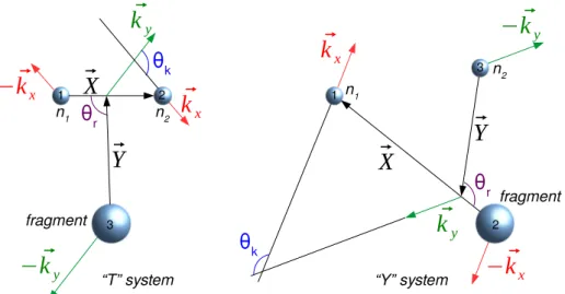
2.8 Two dimensional plot of cos(θnn) as a function of cos(θf /nn) (a) for the18O+n+n events from the simulation of a phase-space decay for Erel =0-12 MeV. The projections over cos(θf /nn) and cos(θnn) are presented in (b) and (c), respectively. 53 2.9 “T” (left) and “Y” (right) Jacobi systems for the fragment+n+n three-body

(12)

2.10 “T” (left) and “Y” (right) Jacobi coordinates of the 18_{O+n+n events from} the simulation of a phase-space decay for Erel =0-12 MeV. The “T” system [Ex/Erel, cos(θk)] coordinates are presented in (a) and (c), respectively and the “Y” system [Ex/Erel, cos(θk)] coordinates in (b) and (d), respectively. . . 56 2.11 (a) Two-neutron correlation function for Erel=3.7-12 MeV of 20O∗ 2n decays.

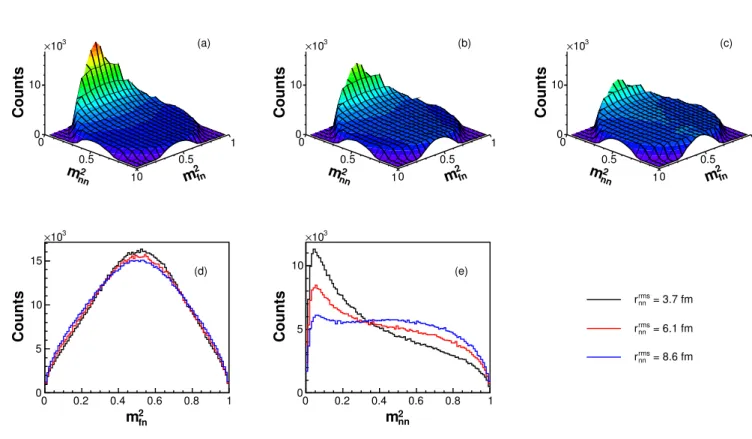
The solid line is traced to guide the eye. (b) Numerator (measured relative momentum distribution, blue points) and denominator (phase space, yellow) of Cnn for the 20O∗ case. . . 56 2.12 (a), (b), (c) Dalitz plots for the 18_{O+n+n direct decay for E}

rel =0-12 MeV from the simulation with a source size of rrms

nn =3.7, 6.1 and 8.6 fm, respectively. The projections onto the normalized invariant masses m2

f n (d) and m2nn (e) are displayed for the three different rrms

nn values. . . 58 2.13 (a), (b), (c) Two dimensional plots of cos(θnn) as a function of cos(θf /nn) for the

18_{O+n+n direct decay for E}

rel=0-12 MeV from the simulation with a source size rrms

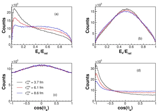
nn =3.7, 6.1 and 8.6 fm, respectively. The projections onto the cos(θf /nn) (d) and cos(θnn) (e) are displayed for three different rnnrms values. . . 59 2.14 “T” (left) and “Y” (right) Jacobi coordinates of the 18_{O+n+n events from the}

simulation of a two-neutron direct decay for Erel =0-12 MeV. The “T” system [Ex/Erel, cos(θk)] coordinates are presented in (a) and (c), respectively and the “Y” system [Ex/Erel, cos(θk)] coordinates in (b) and (d), respectively. The re-sults of three different source sizes rrms

nn are presented. . . 60 2.15 (a) Two-neutron correlation functions and (b) relative momentum distribution

(numerator of Cnn) and phase space (denominator of Cnn in yellow) for the 18_{O+n+n direct decay for E}

rel=0-12 MeV from the simulation for three different source sizes rrms

nn . Lines has been added in (a) with the only purpose to guide the eye. . . 60

2.16 (a), (b), (c) Dalitz plots of the18_{O+n+n sequential decay for E}

rel =5.3-7.2 MeV from the simulation for Er =0.5 MeV, Er =1.5 MeV and Er =2.5 MeV, respec-tively (rrms

nn =6.1 fm and Γr =0.5 MeV being fixed). The projections onto the normalized invariant masses m2

f n (d) and m2nn(e) are displayed for three different Er values. . . 61 2.17 (a), (b), (c) Dalitz plots of the18_{O+n+n sequential decay for E}

rel =5.3-7.2 MeV from the simulation for Γr =0.5 MeV, Γr =1.5 MeV and Γr =3.5 MeV, respec-tively (rrms

nn =3.9 fm and Er =1.5 MeV being fixed). The projections onto the normalized invariant masses m2

f n (d) and m2nn(e) are displayed for three different Γr values (the black curve here corresponds to the red curve in Fig. 2.16). . . 62 2.18 (a), (b), (c) Two dimensional plots of cos(θnn) as a function of cos(θf /nn) for

the 18_{O+n+n sequential decay for E}

rel =5.3-7.2 MeV from the simulation with Er =0.5 MeV, Er =1.5 MeV and Er =2.5 MeV, respectively (rnnrms =6.1 fm and Γr =0.5 MeV being fixed). The projections onto the cos(θf /nn) (d) and cos(θnn) (e) are displayed for three different Er values. . . 63 2.19 (a), (b), (c) Two dimensional plots of cos(θnn) as a function of cos(θf /nn) for

the 18_{O+n+n sequential decay for E}

rel =5.3-7.2 MeV from the simulation with Γr =0.5 MeV, Γr =1.5 MeV and Γr =3.5 MeV, respectively (rnnrms =3.9 fm and Er =1.5 MeV being fixed). The projections onto the cos(θf /nn) (d) and cos(θnn) (e) are displayed for three different Γ values. . . 64

(13)

2.20 “T” (left) and “Y” (right) Jacobi coordinates of the 18_{O+n+n events from} the simulation of a two-neutron sequential decay for Erel =5.3-7.2 MeV with rrms

nn =6.1 fm and Γr =0.5 MeV. The “T” system [Ex/Erel, cos(θk)] coordinates are presented in (a) and (c), respectively and the “Y” system [Ex/Erel, cos(θk)] coordinates in (b) and (d), respectively. The results of three different resonance energies Er are shown. . . 65 2.21 “T” (left) and “Y” (right) Jacobi coordinates of the 18_{O+n+n events from}

the simulation of a two-neutron sequential decay for Erel =5.3-7.2 MeV with rrms

nn =3.9 fm and Er =1.5 MeV. The “T” system [Ex/Erel, cos(θk)] coordinates are presented in (a) and (c), respectively and the “Y” system [Ex/Erel, cos(θk)] coordinates in (b) and (d), respectively. The results of three different resonance widths Γ are shown. . . 65

2.22 (a) Two-neutron correlation functions and (b) relative momentum distribution (numerator of Cnn) for the18O+n+n sequential decay for Erel =5.3-7.2 MeV from the simulation with rrms

nn =6.1 fm, Γr =0.5 MeV and three different resonance energy values Er. . . 66 2.23 (a) Two-neutron correlation functions and (b) relative momentum distribution

(numerator of Cnn) for the18O+n+n sequential decay for Erel =5.3-7.2 MeV from the simulation with rrms

nn =3.9 fm, Er =1.5 MeV and three different resonance width Γ values. . . 66

3.1 Nuclei studied during this thesis at RIKEN (blue square) and GSI (red square). The secondary beams used to populate them are also presented in green and black squares for RIKEN and GSI, respectively. . . 69

3.2 Sketch of the general principle used during our experiments. . . 70

3.3 Sketch of the typical detection setup used during our experiments, with the beam traveling from left to right. It is first going through beam trackers in order to reconstruct its trajectory before reaching the reaction target, which is surrounded by a γ-ray detector to detect eventual in flight γ rays. After the reaction, the emitted neutron(s) go straight into a neutron detector where their trajectory and time of flight are measured, while the charged fragment, deflected by a magnet, is detected and identified using a set of detectors allowing us to reconstruct its trajectory and energy loss. . . 71

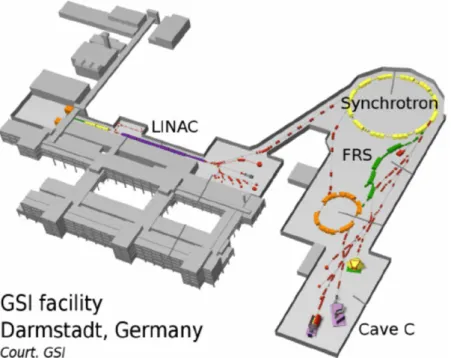
3.4 Schematic layout of the GSI accelerator complex used during the experiment. . . 72

3.5 Sketch of the FRS. The Bρ-∆E-Bρ method is applied using dipoles to bend the beam (Bρ) as well as a degrader to have a position and Z-dependent energy loss (∆E) (figure taken from [6]).. . . 73

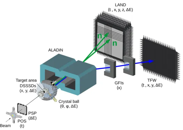
3.6 Experimental setup in Cave C as used during the s393 campaign. The observables measured by each detector are presented in parenthesis. . . 74

3.7 Identification of the nuclei in the cocktail beam. . . 75

3.8 Identification of the fragments produced from the interaction of19_{N nuclei from} the beam with the target. The charge identification is presented of the left panel and the mass identification for the Carbon isotopes is presented on the right panel. 77

(14)

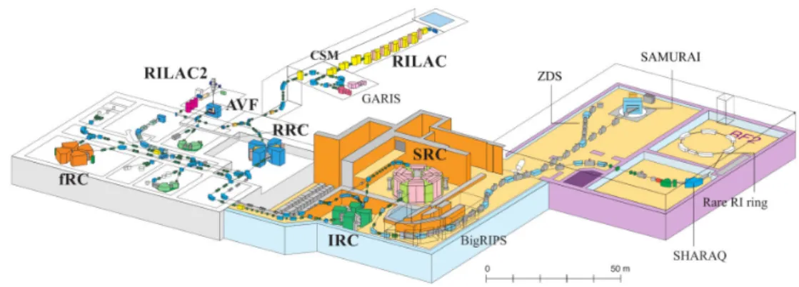
3.9 Sketch of the RIBF facility at RIKEN. During the SAMURAI 21 experiment, the 48_{Ca stable beam has been accelerated from the linear accelerator RILAC} to the cyclotron SRC. After fragmentation on the Be target, the radioactive beam was selected using the BigRIPS fragment separator before being sent to the SAMURAI experimental area. . . 78

3.10 Sketch of the BigRIPS fragment separator. The different dipoles are labeled from D1 to D7 and the quadrupoles allowing the focusing of the beam are labeled from STQ1 to STQ25. . . 79

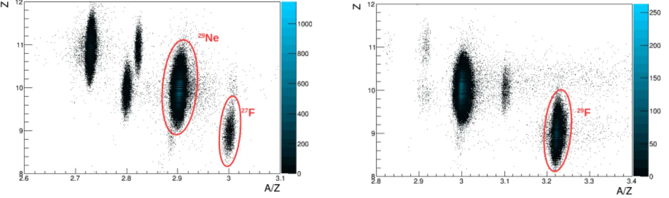
3.11 Identification of the cocktail beam for the two different settings used in the SAMURAI21 experiment. . . 80

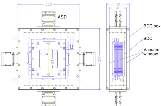
3.12 Sketch of a Beam Drift Chamber (BDC). The dimensions are displayed in mm. . 81

3.13 Sketch of the MINOS device.. . . 81

3.14 Sketch of a FDC1 drift chamber. The dimensions are displayed in mm. . . 83

3.15 Sketch of a FDC2 drift chamber. The dimensions are displayed in mm. . . 84

3.16 Identification of the charged fragments produced from a 29_{Ne (left) and} 29_F (right) beam after its interaction with the MINOS target. . . 84

3.17 Test of the DALI2 simulation on the γ-ray transition from 27_F∗_{. The data (black} points) are fitted using a distribution (black line) with two components: the result of the simulation (red dashed line) and a exponential (blue dashed line). . 86

3.18 Superposition of the beam velocity distributions from the data (red) with the distribution given as an input of the simulation (black) for the (29_F,27_F+n) reaction channel. . . 87

3.19 Superposition of the angular distributions obtained for different ions by selecting a pencil beam on the empty target and the function used in the simulation to reproduce those distributions. . . 89

3.20 Distributions of total momentum obtained for the 29_F, 29_Ne,30_{Ne pencil beams.} The black curve represent the best compromise obtained to reproduce the three distributions using only one Gaussian. In each case, the simulation is normalized to the data so that their integrals match. . . 90

3.21 On the left, evolution of the geometrical acceptance for the neutron detection in the SAMURAI21 experiment (NeuLAND and NEBULA) as a function of the relative energy of a fragment+n resonance formed at 230 MeV/nucleon. On the right, evolution of the geometrical acceptance for the neutron detection in NeuLAND (blue) and NEBULA (red). . . 91

3.22 Evolution of the experimental resolution in the SAMURAI21 as a function of the fragment-neutron relative energy for a beam at 230 MeV/nucleon. The red line on the right characterizes the evolution of the resolution. . . 92

3.23 Effects of the cross-talk rejection procedure of the true 2n events using MANGA. We show the superposition of the detection efficiency curves before (blue) and after (red) the cross-talk rejection algorithm as a function of the relative energy. 93

3.24 On the left, relative energy spectrum obtained for the 29_F(p,pn)28_{F reaction in} the SAMURAI21 experiment to which the maximized non-resonant contribution has been added (red). On the right, ratio of the relative energy by the maximized non-resonant contribution for the same reaction channel. . . 94

(15)

3.25 On the left, χ2 _{surface obtained by adjusting the relative energy spectrum for} the first peak observed in the 29_F(p,pn)28_{F reaction. Each area corresponds to} five units of χ2_{. The energy is varying from 0.15 to 0.25 MeV and the width} from 0.01 to 0.3 MeV. On the right, result for the best fit of the same spectrum. 95

3.26 Projections of the χ2 _{surface on the resonance energy (E}

r) and width (Γr). The red line corresponds to the limit χ2 _{≤ χ}2

min+ 10 . . . 95

4.1 Gamma rays observed in coincidence with the reaction19_N(p,2p)18_C∗_{. The data} are fitted with an exponential component as well as three Gaussian functions. . 98

4.2 Relative energy obtained for the 19_N(p,2p)18_C∗ _→17_{C+n reaction. The data} are fitted using two ℓ-dependent Breit-Wigner functions (green and blue dashed lines) where the response of the experimental setup is taken into account. The total fit (red line) has been found to be the best with ℓ=1 for the lower-energy resonance and ℓ=0 for the higher-energy one. The blue histogram represents events in coincidence with known γ-rays in17_{C taking into account the efficiency} of the γ-ray detector. . . 99

4.3 Gamma rays observed in coincidence with the 19_N(p,2p)18_C∗ _→17_{C+n reaction.} The data are fitted with an exponential component as well as a Gaussian function.100

4.4 Illustration of the shell-model configuration of the 12 neutrons in the 18_{C (left)} and20_{O (right) isotones. In the (p, 2p) reaction the configuration of the neutrons} is unchanged and all neutrons are likely paired, while in the (p, pn) reaction two neutrons are left unpaired. . . 101

4.5 Experimental decay energy spectra of16_{C+n+n and}18_{O+n+n measured} respec-tively in the proton/neutron knockout reactions from 19_N/21_{O (blue histograms} represent events in coincidence with known γ rays in16_C/18_{O, corrected by ε}

γ). The corresponding locations of the 2n and 4n thresholds are noted. . . 102

4.6 Comparison between the Erel of three different systems. The 21_O(p,pn)20_O→18_{O+2n system in black and the} 19_N(p,2p)18_C→16_C+2n system in red from Fig. 4.5, and the 16_C(p,2p)15_B→13_{B+2n system in blue.} _{. . . 103} 4.7 γ-ray spectra observed in coincidence with the 18_C→16_{C+2n channel for two}

different gamma multiplicities (Mγ).. . . 104 4.8 Dalitz plots of fragment+n+n decays (fragment-n vs n-n normalized squared

in-variant masses). Left panels correspond to16_{C+n+n, right panels to} 18_O+n+n. The four upper panels represent simulations of (a) phase space, (b) sequential decay through a fragment-n resonance, (c) direct decay with n-n FSI, and (d) a combination of the latter two. The lower panels (e,f) correspond to the experi-mental data for the relative energies noted. . . 105

4.9 Projection of the Dalitz plots defined in Fig. 4.8 onto either axes for the data of 18_C∗ _{(left) and} 20_O∗ _{(right) decays. The rows correspond to the four E}

rel bins defined in the text, from lower (top) to higher (bottom). The yellow histograms represent phase space, normalized to the data at m2

nn> 0.6. The red histograms are the projections of the best two-dimensional fit of the plots, with their direct (green) and sequential (purple, with percentage noted) decay components. . . . 106

(16)

4.10 (a) Two-neutron correlation functions from the three higher-energy bins of 18_C∗ (blue) and 20_O∗ _{(red) 2n decays. The solid lines are traced to guide the eye,} while the dashed lines correspond to the fits of the experimental data from the breakup of 14_{Be (green) [}₇_{] and the neutron evaporation from} 44_{Ca (black) [}₈_]. (b) Numerator (measured relative momentum distribution, blue points) and de-nominator (phase space, yellow) of Cnn for the 18C∗ case. . . 107 4.11 Comparison between the Dalitz plot for 18_{C obtained with the data (left) and}

the one obtained from the simulation for the best fit (right). The comparison for different Erel ranges are shown: Erel =0-3.7 MeV for (a) and (b), Erel =3.7-5.3 MeV for (c) and (d), Erel=5.3-7.2 MeV for (e) and (f) and Erel =7.2-12 MeV for (g) and (h). . . 108

4.12 Comparison between the Dalitz plot for 20_{O obtained with the data (left) and} the one obtained from the simulation for the best fit (right). The comparison for different Erel ranges are shown: Erel =0-3.7 MeV for (a) and (b), Erel =3.7-5.3 MeV for (c) and (d), Erel=5.3-7.2 MeV for (e) and (f) and Erel =7.2-12 MeV for (g) and (h). . . 110

5.1 Relative energy spectrum obtained for the 27_F(p,pn)26_{F reaction in the} SAMU-RAI21 experiment (black). The relative energy spectrum obtained for the same reaction in the DAYONE experiment (without the MINOS target and without the NeuLAND detector) is also shown (red). . . 114

5.2 On the left, relative energy spectrum obtained for the 27_F(p,pn)26_{F reaction in} the SAMURAI21 experiment to which the maximized non-resonant contribution as been added. On the right, ratio of the relative energy by the maximized non-resonant contribution for the same reaction channel. . . 115

5.3 Best fit obtained for the relative energy spectrum of the 27_F(p,pn)26_{F reaction.} The resonances are numbered as R₁₋₆. . . 115

5.4 On the left, decomposition of the γ-ray spectrum of 25_{F. The solid black line} shows the final fit which includes the response function from GEANT4 simulation (green solid curves) and the additional exponential background plotted as dashed red line. On the right, proposed level scheme of 25_{F compared to shell-model} calculations performed using USD, USDA and USDB interactions. Energies are given along the transitions as well as their relative intensities in italics. Both figures are taken from [9]. . . 116

5.5 γ-ray spectrum obtained in coincidence with 25_{F+n events.} _{. . . 117} 5.6 Upper panel, relative energy gates for the 25_{F+n events corresponding to the}

R₁₋₆resonances. Lower panel, γ-ray spectra corresponding to each gate (match-ing colors) presented in the upper panel. . . 118

5.7 Inclusive parallel-momentum distribution of the fragment (26F) in the beam rest frame detected during the 27_F(p,pn)26_F(∗) _{reaction. Eikonal-model theoretical} calculations are shown in different colors in order to compare them to the exper-imental distribution. . . 119

5.8 Parallel-momentum distribution for the R₁₋₄resonances of the (25_{F+n) unbound} system in the beam rest frame. Eikonal-model theoretical calculations are shown in different colors in order to compare them to the experimental distribution. . . 120

(17)

5.9 Proposed level scheme of 26_{F deduced from our experimental results for the} 27_{F(−1n) reaction.} _{. . . 121} 5.10 On the left, relative-energy spectrum obtained for the 29_Ne(p,2p)28_{F reaction in}

the SAMURAI21 experiment to which the maximized non-resonant contribu-tion has been added (red). On the right, ratio of the relative energy and the maximized non-resonant contribution for the same reaction channel. . . 121

5.11 Superposition of the relative-energy spectra for the27_{F+n system obtained when} the neutron is detected in NeuLAND (black) or NEBULA (red). . . 122

5.12 On the left, best fit obtained for the relative-energy spectrum for the 27_F+n system. On the right, same figure in logarithmic scale. . . 122

5.13 γ-ray spectrum obtained in coincidence with 27_{F+n events. The data (black} points) are fitted using a distribution (black line) with two components: the result of the simulation (red dashed line) and an exponential (blue dashed line). 123

5.14 Upper panel, relative energy gates for the 27_{F+n events. Lower panel, γ-ray} spectra corresponding to each gate (matching colors). . . 124

5.15 Proposed level scheme of 28_{F deduced from our experimental results for the} 29_{Ne(−1p) reaction.} _{. . . 125} 5.16 On the left, relative energy spectrum obtained for the 29_F(p,pn)28_{F reaction in}

the SAMURAI21 experiment to which the maximized non-resonant contribution has been added (red). On the right, ratio of the relative energy by the maximized non-resonant contribution for the same reaction channel. . . 126

5.17 γ-ray spectrum obtained in coincidence with 27_{F+n events.} _{. . . 126} 5.18 Upper panel, relative-energy gates for the 27_{F+n events. Lower panel, γ-ray}

spectra corresponding to each gate (matching colors). . . 127

5.19 On the left, best fit obtained for the relative energy spectrum for the 27_F+n system populated from 29_{F(−1n). On the right, same figure in logarithmic scale.} ₁₂₈ 5.20 Proposed level scheme of 28_{F deduced from our experimental results for the}

29_{F(−1n) reaction.} _{. . . 129} 5.21 Parallel-momentum distribution for the R1 resonance (0.20 MeV) of the 27F+n

unbound system populated from 29_{F(−1n) in the beam rest frame.} Eikonal-model theoretical calculations are shown in different colors in order to compare them to the experimental distribution. The area in which theoretical and exper-imental distributions are compared is shown in red. . . 130

5.22 Parallel-momentum distribution for the R3 resonance (1.00 MeV) of the 27F+n unbound system populated from 29_{F(−1n) in the beam rest frame.} Eikonal-model theoretical calculations are shown in different colors in order to compare them to the experimental distribution. The area in which theoretical and exper-imental distributions are compared is shown in red. . . 131

5.23 Relative energy for one and two neutrons decay channels of 28_{F populated from} 29_{Ne(-1p). On the left, the S}

n(27F) value considered is the one from the AME2016 evaluation. On the right the Sn(27F) value is 1600 keV. . . 132 5.24 Superposition of the relative-energy spectra for the 26_{F+2n system populated}

from 29_{Ne(-1p) when the two neutrons are detected in NeuLAND (black), the} two neutrons are detected in NEBULA (red) and one neutron is detected in each detector (blue). The distributions are normalized to the red curve to facilitate the comparison. . . 133

(18)

5.25 Relative-energy spectrum for the 26_{F+2n system populated from}29_{Ne(-1p) with} a gate such as 0.4 < m2

f n < 0.6. . . 133 5.26 Relative-energy spectrum for the 26_{F+2n system populated from} 29_Ne(-1p). _{. . . 134} 5.27 On the upper panel, the gates applied to construct the Dalitz plots are

repre-sented on the relative-energy spectrum for the 26_{F+2n system populated from} 29_{Ne(-1p). On the lower panel, the Dalitz plots are presented for the red and the} blue gates on the left and right, respectively. . . 135

5.28 Proposed level scheme of 28_{F deduced from our experimental results for the} 26_{F+2n system.} _{. . . 136}

6.1 On the left, level scheme summarizing the states observed in 28_{F. On the right,} proposed parabolas for the lower energy states observed in 28_F. _{. . . 141} A.1 Sketch of the alignment procedure for the drift chambers (figure taken from [5]).

The position measured in BDC2 is compared to the one interpolated from BDC1 and FDC1.. . . 143

A.2 Measurement of the relative alignment of the drift chambers. The graphs rep-resent the difference between the measured position in BDC2 and interpolated position from BDC1 and FDC1 for a 29_{Ne beam on empty target.} _{. . . 144} A.3 Drift time inside the TPC during a physics run. . . 145

A.4 Evolution of the drift velocity as a function of the run number during the SAMU-RAI21 experiment. . . 146

A.5 zvertex distribution for an empty target run.. . . 146 A.6 TDC distribution of the first wire plane of BDC1. . . 149

A.7 Schematic view of the position of the HPC around NEBULA (figure taken from Ref. [5]). . . 153

A.8 Distribution of the measured time in the bar number 315 of NeuLAND. . . 154

A.9 ToF of the measured particles in NeuLAND as a function of the bar ID. . . 154

A.10 Fragment-n alignment procedure for the 29_F→ 27_{F+n reaction channel. Each} figure represents the evolution of an observable as a function of the fragment velocity shift ∆βf. . . 156 A.11 Space-time distribution of the hits detected for the29_Ne→27_{F+n reaction}

(19)

(20)

List of Tables

1.1 Experimental and calculated interaction energies, Int(J), between a πd5/2proton and a νd3/2 neutron in 26F. Calculated results are obtained from USDA and IM-SRG shell-model calculations (adapted from [3]).. . . 36

3.1 Properties of the different plastic scintillators placed on the beam line. The relative distances are given with respect to the middle of the two SBT detectors. 80

4.1 Energies of the γ-ray transitions observed in our experiment for the reaction 19_N(p,2p)18_C∗_{. The results of a previous study are also presented as comparison.} ₉₈ 4.2 Summary of the results obtained from the fitting of the experimental relative

energy for the 19_N(p,2p)18_C∗ _→17_{C+n reaction.} _{. . . 99} 4.3 Table summarizing the parameters obtained from the fits of the four-decay energy

bins of 18_{C shown in Fig. 4.11.} _{. . . 109} 4.4 Table summarizing the parameters obtained from the fits of the four-decay energy

bins of 20_{O shown in Fig. 4.12.} _{. . . 109} 5.1 Parameters obtained for the best fit of the relative energy spectrum of the

27_F(p,pn)26_{F reaction.} _{. . . 116} 5.2 On the left, parameters obtained for the best fit of the relative energy spectrum of

the 27_{F+n system populated from} 29_{F(−1n). On the right, parameters obtained} for the best fit of the relative energy spectrum of the 27_{F+n system populated} from29_{Ne(−1p) are recalled in order to facilitate the comparison.} _{. . . 129} A.1 List of the γ-ray sources used for the calibration of DALI2. . . 148

(21)

(22)

Chapter 1 Introduction

N

uclear physics is not a new science. However, after almost one century of research, theatomic nucleus is still not fully understood and new unexpected properties are emerging frequently. Trying to understand the structure and the evolution of the nucleus depending on its constituents is one of the fundamental goals of nuclear physics. Nevertheless, describing the interaction between nucleons is extremely hard to achieve, even for light nuclei where the number of nucleons is small.

Historically, fundamental properties of the nucleus have been investigated by reducing the N-body problem to independent nucleons located in a mean field built in an auto-coherent way. This approach allowed to explain several phenomena observed experimentally such as the magic numbers associated to certain configurations of nucleons particularly stable, and lead to the shell model of the nucleus.

However, even if the stable nuclei are the most abundant on earth, their diversity (nearly

300) represents only a small fraction of the existing nuclei (see Fig. 1.1). Today, nearly 3000

nuclei have been observed experimentally and it is expected that the same amount still remains to be observed. Those nuclei have a limited lifetime after which they decay mainly via β decay. For a given Z number, the more (or the less) neutrons we count away from the equilibrium

(23)

value, and the less stable the nucleus becomes, until reaching a threshold where even in its ground state the nucleus is not bound anymore and decays in a very short time by emitting nucleons. This limit is called neutron dripline (or proton dripline, respectively) and the nuclei around this region usually exhibit very different behavior compared to the stable nuclei.

Figure 1.1: Chart of the nuclides representing with black squares stable nuclei, light yellow neutron-rich or neutron-deficient nuclei already produced in terrestrial laboratories, and in light blue nuclei not studied yet. The limits of proton and neutron particle stability (or driplines), predicted by theoretical models, are shown with red and blue lines, respectively.

One of the major research goals of modern nuclear physics is to explore those regions where the neutron to proton imbalance is reaching extreme values in order to determine the exact position of the dripline. Studying the properties of the nuclei in those regions gives us information on the evolution of their structure while approaching (sometimes even crossing) the limits of existence. The results obtained can then be compared to existing theoretical models and if needed, used to correct or justify the development of new models. A single look

at Fig.1.1 shows the huge work that still needs to be done, in particular around the neutron

dripline. Indeed, the neutron dripline has been reached experimentally only for nuclei with a proton number Z lower than ten.

In this document, we will be investigating the nucleon-nucleon interaction toward the neutron dripline. In practice, the dripline can be reached by changing the proton to neutron ratio but also by increasing the excitation energy of a nucleus beyond the nucleon(s) emission thresholds. This work can be divided in two studies: the n-n interaction in the core+xn systems and the evolution of the p-n interaction in the Fluorine isotopic chain. Indeed, we

(24)

and 20_{O (that can be seen as} 14_{C+4n and} 16_{O+4n, respectively). And we will then study the}

evolution of the p-n interaction in the Fluorine isotopic chain by comparing results from 26_F

and 28_{F, the latter being an unbound system. All the nuclei, be there bound or unbound, are}

studied using knockout reactions, meaning that a nucleon is removed from a nucleus in order to populate the system of interest.

This document is divided in five chapters. In the first one, we will present the particularities of the study of nuclei at the neutron dripline as well as the motivations of such studies. We will then describe the different techniques and observables used in order to explore unbound states. In a third chapter, we are presenting the experimental principle and setups used during this work in order to populate the nuclei of interest as well as the simulations used to understand and interpret the data. In the fourth chapter, we are presenting our results and interpretation

on the n-n pairing in unbound states of 18_{C and} 20_{O. And finally, in the last chapter, we are}

presenting our results and interpretation on the evolution of the p-n interaction in the Fluorine

isotopic chain between 26_{F and} 28_F.

1.1 Toward the neutron dripline

1.1.1 General properties of nuclei

In this section, we are focusing on the description of the lightest nuclei Z ≤ 10. Since we will be investigating those nuclei, we start by describing the characteristics of stable nuclei before comparing them to those of neutron-rich ones.

Despite a limited number of isotopes for each chemical element, light nuclei can be very different from each other. Stable nuclei have the following characteristics:

• The N/Z ratio between their number of neutrons and protons varies slightly varying around 1.

• The binding energy between the nucleons is similar for all the nuclei and is around

8 MeV/nucleon. The separation energies for one proton (Sp) or one neutron (Sn) are

also very similar.

• Their radius can be described by the empirical formula R = r0A1/3 [10], where r0 is

the effective radius of a nucleon (r0 ≈1.2 fm) and A is the total number of nucleons.

Such description assumes an homogeneous distribution of the nucleons in the nucleus (independently of their nature).

• The presence of several bound excited states. Those states, whose excitation energies vary from one isotope to the other, usually decay by the emission of γ-rays.

While moving away from stability those properties change rapidly and nuclei become unstable, with shorter and shorter lifetimes. If the lifetime of the nuclei close to stability is varying from a few years to a few seconds, the lifetime of the neutron rich nuclei is dropping rapidly under the second and they survive only a few milliseconds approaching the dripline. The N/Z ratio for nuclei outside the valley of stability can vary from 0.6 to 4 and their

(25)

separation energies Sn,p vary from 40 to 0 MeV [11].

When the ratio reaches extreme values, the radial distributions of protons and neutrons can decouple massively and give raise to exotic phenomena such as the neutron halo: in those nuclei, the radial distribution of neutrons shows a tail that spreads much further than the proton one. Those nuclei can therefore be represented as a light core around which one or several neutrons are orbiting. A similar phenomenon can be observed for proton halos in the case where N/Z is very low. However, in that case this manifestation is less obvious due to the Coulomb bar-rier that does not allow protons to have a spatial wave function as spread as the one of neutrons. In our study, we are interested by the light neutron-rich nuclei and in particular nuclei that

have such a large excess of neutrons that are unbound (28_{F). For a stable nucleus, the proton}

and neutron potentials have similar characteristics, except for the Coulomb contribution, that makes the proton potential less deep. If the number of neutrons increases, the proton potential

becomes deeper due to the attractive n-p interaction [11]. Therefore the separation energy for

the protons becomes larger while the one for the neutrons becomes smaller, its value reaching zero close to the dripline.

Moreover, bound excited states become more and more rare while moving toward the neutron dripline. The last bound isotopes of an element usually do not have any bound excited state. This is why the study of neutron-rich nuclei usually requires to do spectroscopy of unbound states.

1.1.2 Structure in nuclear physics

Nuclei, like all the subatomic particles, follow the rules of quantum mechanics. In particular, their evolution is governed by the Shr¨odinger equation. Considering the simple case of a particle with mass m in a potential depending only on its position, the Shr¨odinger equation can be written as follows [12]: − ~ 2 2m∆ψ(~r, t) + V (~r)ψ(~r, t) = i~ ∂ψ(~r, t) ∂t (1.1)

where V (~r) is the potential in which the particle is and ψ(~r, t) its wave function. In the case of a problem with several particles interacting with each other, the problem is more complex since the potential felt by each particle is a function of the state of all the others. This interdependence is known as the N-body problem and is encountered in numerous fields of physics. The complexity of this problem increases with the number of particles. It is possible to solve it analytically for very small number of particles but it remains unsolvable exactly in its general case. We therefore solve it numerically using different methods that have been developed. We can give as example for light nuclei the techniques called ab initio: NSCM (No Core Shell Model), GFMC (Green Function Monte Carlo), Coupled Cluster... However, those different techniques encounter sometimes different problems that can be conceptual or due to numerical convergence.

Another difficulty, proper to nuclear physics, adds itself to the problem: there is no analytic form for the interaction potential between two nucleons inside a same nucleus fundamentally

(26)

speaking. Quantum chromodynamics [13] is the theory that studies, in a fundamental level, the strong interaction that confines the quarks inside the nucleus. This theory allowed to treat problems up to four nucleons but shows some numerical limitations when the systems become more complex. Moreover all the models used in nuclear physics are based on effective interaction potentials.

Historically, the model that encountered a big success and allowed us to better understand nuclei is the model of independent particles. In this model, particles are considered entirely independent one from another and are sitting in a mean potential (also called mean field). In this context, we can express the wave function of the system such as the sum of the wave functions of each independent particle that composes the system. The Hamiltonian of the system can be expressed as follows:

ˆ H = N X i=1 ˆ Ti+ N X i=1 N X j>i ˆ Vij ≈ N X i=1 ˆ Ti+ ˆUi (1.2)

where ˆH is the Hamiltonian of the system, ˆTi is the kinetic part associated to the particle i,

ˆ

Vij the interaction potential between particles i and j, and ˆUi the effective potential felt by

particle i.

Considering that the potential has spherical symmetry and by adding the spin-orbit term,

it is possible to show [12] that the energy levels of the system can be obtained as the sum

of the energies enlj of the independent particles. Those energies enlj are obtained using the

diagram presented in Fig.1.2. Each combination of quantum numbers n, l and j characterizes

what is called an orbital. The latter can contain at most 2j+1 nucleons with the same energy, depending on the orbital. The total energy is obtained by filling the orbitals with the nucleons of the system. In this model, neutrons and protons are decoupled and are filling a similar diagram independently. To build those diagrams, we order the orbitals from the lower to the higher energy, so that an independent particle located on a higher orbital has systematically more energy than any other particle located in a lower orbital. The nucleons of the last occupied orbital are called valence nucleons, the others being sometimes called core nucleons.

In this model, the ground state of a nucleus is obtained by minimizing the total energy, i.e. by following the order of the orbitals while filling them with the nucleons of the nucleus of interest. In order to obtain the different excited states of a nucleus, one needs to modify the ground-state configuration by promoting one or several valence nucleons into higher orbitals. To distinguish the different configurations, we are using in this entire document the following notation:

π(nlj)Np_{⊗ ν(nlj)}Nn_,

where π(nlj) and ν(nlj) depict the valence protons and the valence neutrons, respectively

and Np and Nn how many of them are located in those orbitals. All the lower orbitals

be-low the valence ones are supposed to be fully filled, which albe-lows the use of a condensed notation. There are pairing effects between nucleons of a same orbital that tend to lower their individual energy when they are paired. This effect is directly visible by looking at the nuclear

(27)

Figure 1.2: Energy levels of a model with independent particles. Each level (also called orbital) is characterized by the quantum numbers nlj. The orbitals are classified from bottom to top by increasing energy. The numbers between orbitals correspond to the number of nucleons used if all the lower energy orbitals are filled.

neutron dripline: some isotopes with an even number of neutrons are bound while isotopes with one neutron less are unbound.

The historical model that has been used to reproduce the nuclei from the valley of stability

using the assumption of independent particles is the shell model [14]. It allows to derive in

particular the so called magic numbers. Nuclei with a magic number of nucleons (2, 8, 20, 28, 50, 82, 126) show singular properties that have been observed experimentally. For example,

Fig. 1.4 shows the evolution of the neutron separation energy (Sn) for nuclei with an even

number of neutrons as a function of their neutron number. We observe sharp drops at each magic number (in particular for 50, 82 and 126), meaning that it is much harder to remove a neutron when the neutron number corresponds to a magic number.

In the diagram presented in Fig. 1.2, the magic numbers correspond to the number of

nucleons necessary to fill entirely certain orbitals: 1s1/2, 1p1/2, 1p3/2... Those orbitals are characterized by an important separation energy compared to the orbital above, meaning that transferring a nucleon to the next orbital would cost a lot of energy.

However, this simple model shows its limits while moving away from stability. The sepa-ration energy between two orbitals and even their order can change while moving toward the neutron dripline. If we take as an example the Oxygen isotopic chain, several experimental

(28)

1 H 2H 3 He 4He 7 Li 6 Li 7 Be 9Be 11_B 10_B 13_C 12_C 15_N 14_N 16_O 17_O 18_O 19 F 20 Ne 21Ne 22Ne 23 Na 5 He 7He 10 Li 12Li 13 Be 8 Be 9_B 9_B 16_B 18_B 21_C 24_N 25_N 25_O 26_O 27_O 28_O 28 F 30F 33 Ne 36 Na 1 n 3 H 8 He 9 Li 8 Li 10 Be 11Be 12Be 12_B 13_B 14_B 15_B 14_C 15_C 16_C 17_C 18_C 19_C 20_C 16_N 17_N 18_N 19_N 20_N 21_N 22_N 23_N 19_O 20_O 21_O 22_O 23_O 24_O 20 F 21F 22F 23F 24F 25F 26F 27F 29F 31F 23 Ne 24Ne 25Ne 26Ne 27Ne 28Ne 29Ne 30Ne 31Ne 32Ne 34Ne 24 Na 25Na 26Na 27Na 28Na 29Na 30Na 31Na 32Na 33Na 34Na 35Na 6 He 11 Li 14 Be 17_B 19_B 22_C 8_B 9_C 10_C 11_C 12_N 13_N 13_O 14_O 15_O 14 F 14 F 15F 16F 17F 18F 16 Ne 17Ne 18Ne 19Ne 18 Na 19Na 20Na 21Na 22Na stable β+ β− halo unbound

Figure 1.3: Nuclear chart for light nuclei.

Figure 1.4: Evolution of the neutron separation energy for nuclei with an even number of neutrons

as a function of their neutron number. The arrows located below the horizontal axis correspond to the magic numbers (figure taken from [1]).

the magic number N = 20 disappears [18]. Different theoretical calculations [19, 20] explain

(29)

1.1.3 Unbound nuclei and resonant states

Nuclei close to the dripline are weakly bound and most of the time do not have any bound

excited state. It is the case for example for nuclei such as 6_{He or} 11_{Li, that do not have any}

bound excited states below the two neutron emission threshold (S2n). In this conditions, excited

states can manifest themselves as resonances. Past the dripline, nuclei become unstable with respect to the emission of particles even in their ground state. However, in the case of unbound nuclei located close from the emission thresholds, it is possible to observe resonant states, their lifetime τ being generally associated to the width of the resonance Γ due to the Heisenberg uncertainty principle:

Γ × τ ∼ ~ (1.3)

For an unstable system with respect to the emission of one neutron, the relative energy spectra of the fragment-neutron system can reveal the presence of resonant states. A well

known example is the one of the unbound Helium isotopes. For example 7_{He, which ground}

state has been observed as a resonance since the sixties [21]. The difficulty to observe

those states is that they have very short lifetimes (of the order of 10−21 _{s). As a}

conse-quence, the measurement of the energy of those states can only be done in an indirect way, using reactions, by observing the decay products and/or other particles involved in the reaction. If we consider only the fragment-neutron relative movement during the decay, the apparition of a resonant state depends entirely on the shape of the potential felt by the neutron. For a neutron with an angular orbital ℓ, the effective potential is given by [22]:

Vef f(r) = VN(r) + Vℓ(r) = VN(r) +

~2_{ℓ(ℓ + 1)}

2µr2 (1.4)

where r is the fragment-neutron distance, µ the reduced mass, VN the attractive nuclear

potential created by the fragment and Vℓ the repulsive centrifugal potential, that depends

quadratically on the angular momentum. The larger is the angular momentum ℓ, the higher is the centrifugal barrier, which implies the confinement of the neutron in the potential for a longer time since the penetrability of the barrier is inversely proportional to its height

[23]. As a consequence, for ℓ > 0, we obtain resonant states which lifetime τ increases

(and width decreases) with a larger ℓ. But for neutrons with angular momentum equal

to zero, the contribution from the Vℓ term disappears and there is no more centrifugal

barrier (see Fig. 1.5). It is therefore impossible to observe resonant states in that case.

How-ever, if an increase of the cross-section is observed toward 0 energy, we talk of virtual states [24]. In fact, such a description is too simple, since only the relative fragment-neutron movement is taken into account and that no assumption is made on the internal structure of the fragment. Indeed, models that take into account the coupling between the different configuration of the

fragment predict the existence of an ℓ = 0 resonance [1]. However this simple vision allows us

to obtain information on the structure of unbound states.

In this description, resonant and virtual states are treated like the diffusion of a neutron on

the fragment. The differential cross-section in relative energy (Erel) for a partial wave with an

angular momentum ℓ can be expressed as follows: dσℓ dErel = 4π k2 rel (2ℓ + 1) sin2_δ ℓ(Erel) (1.5)

(30)

Figure 1.5: On the left, effective potential felt by a neutron with an ℓ > 0 angular momentum. We notice that it shows a centrifugal barrier (in dashed blue line) that can confine the neutron and induce the formation of resonant states that can be observed. On the right, case where ℓ = 0, no centrifugal barrier is felt by the neutron. The insets on the top right of each figure represent the kind of differential cross-section in relative energy that we obtain in each case.

where krel is the wave number linked to the fragment-neutron relative momentum and δℓ is

the phase of the wave ℓ induced by the potential on the neutron wave function. In the case of a resonance with ℓ > 0, the phase will be negligible for all the partial waves except for

the resonant ℓ component. The cross-section will display a maximum at an energy Er with a

width Γ. In that case, the shape of the phase in Eq. 1.5 leads to a Breit-Wigner distribution

and the two parameters Er and Γ allow to entirely characterize the unbound state.

For virtual states, at low energy, it is possible to link the phase with the scattering length as. This parameter gives us a measurement of the attractive potential ability to bind the system:

it is positive for bound states and negative for unbound states. At very low energy (krel→ 0),

we can do the following approximation:

δ0 ≈ −askrel (1.6)

In such conditions, the cross-section displays a maximum very close from the neutron emis-sion threshold, with a tail that spreads to higher energies (see Fig.1.5). We can link qualitatively the scattering length to the corresponding resonance energy using the following approximation [25]: Er ≈ ~2 2µa2 s (1.7)

We obtain therefore for example that a scattering length as =-20 fm corresponds to a

resonance energy of about Er =50 keV for A∼9. However this formula can be used only

(31)

1.2 The nucleon-nucleon interaction inside the nucleus

1.2.1 General properties of the nucleon-nucleon interaction

We present here the general properties of the nucleon-nucleon interaction in a qualitative way. The intensity of the interaction between two nucleons depends on several parameters:

• The strongest intensity for the interaction is obtained when the wave functions of the two nucleons show the larger spatial overlap. This is happening when two nucleons have the same number of nodes (characterized by the quantum number n) and the same angular orbital momentum ℓ.

• The nuclear interaction depends on the spins of the nucleons. The proton-neutron inter-action, in particular, is the largest for a proton and a neutron with anti-aligned spins for

ℓ 6= 0, i.e. for s1 = 1/2 and s2 = −1/2. For example, the proton-neutron πd5/2⊗ νd3/2

interaction will be stronger than the πd5/2⊗ νd5/2 interaction.

• Empirically, it has been shown that the intensity of the nuclear force inside a nucleus is

inversely dependent on the size of the nucleus. This dependence is a function of A−1/3 _or

A−2/3 _{depending whether the nucleons are located at the surface or at the center of the}

nucleus. We can understand it qualitatively from the fact that when the size increases, nucleons ‘meet’ less often, decreasing therefore their interaction which has a short range. An important consequence from this decreasing of the nuclear interaction when the size of the nucleus increases is that the modification of the nuclear structure will occur much faster in light nuclei compared to heavier ones.

• Since the nucleus is made of neutrons and protons, there are two isospin values: T=0 and T=1. However, the T=0 value can be obtained only for a proton-neutron system while the T=1 value can be obtained for proton-proton, proton-neutron or neutron-neutron system. The effective interaction will therefore be stronger for a proton-neutron system than for a system with two identical nucleons.

1.2.2 Empirical determination of the proton-neutron interaction

The proton-neutron interaction, for given orbitals, can be obtained experimentally from the structure of odd-odd nuclei (odd number of protons and odd number of neutrons). We also need to assume that the chosen nucleus can be seen as an inert core to which only

one neutron and one proton are added. This method can therefore only be applied to

nuclei with a core possessing a strong shell closure. Indeed in that case, the core excita-tions are at very high energy and their influence on the valence proton and neutron is negligible.

We can take as an example the 38_{Cl nucleus. It can be seen as a} 36_{S doubly-magic core}

on top of which a proton is added in πd3/2 and a neutron in νf7/2. The coupling of those two

nucleons gives four negative parity states with spin Jπ _{= 2}−_{, 3}−_{, 4}−_{, 5}−_{. We will now determine} their binding energy (BE) resulting from adding independently one proton and one neutron

to the 36_{S core. Adding one proton in πd}

3/2 gives us 37Cl which binding energy is known.

Therefore we can determine the gain in binding energy resulting from adding a proton in πd3/2

to the 36_{S core:}

(32)

In a similar way, adding one neutron in νf7/2 gives us37S and the resulting binding energy gain can be expressed as follows:

BE(37_{S) − BE(}36S) = Sn(37S) (1.9)

Figure 1.6: Determination of the interaction energy πd_3/2_⊗νf_7/2from the structure of38Cl extracted from [2]. Int(J) are the interaction energies defined as the difference between the reference value BE(38Cl) and the real binding energy of the J spin state. The weighted average of those interaction energies Vpn(d_3/2f_7/2) is an approximation of the monopole energy.

Finally, adding those two terms to the36_{S nucleus binding energy, we obtain the}38_{Cl nucleus}

binding energy assuming that the neutron in νf7/2 and the proton in πd3/2 do not interact with

each other. This can be written such as:

BE(38Clf ree) = BE(36S) + Sn(37S) + Sp(37Cl) (1.10)

Comparing now this value to the binding energies of the four states obtained experimentally

for38_{Cl, we obtain the interaction energy between the proton in πd}

3/2 and the neutron in νf7/2 coupled to a given spin (assuming that the gain in energy is only due to the proton and the neutron that have been added). We note those interaction energies Int(J). The results for 38_{Cl, extracted from [}₂_{], as well as an illustration of the method are presented in Fig.} _1.6_{. We}

then define the weighted average Vpn _{of the interaction energies, called monopole energy. It}

can be expressed in the following way:

Vpn _≈ P j(2J + 1) × Int(J) P j(2J + 1) (1.11)

(33)

In the case discussed here, we have been able to determine the Vpn_(d

3/2f7/2) value that is of about −1 MeV, which is close from the value predicted by shell-model calculations (-1.19 MeV). The monopole interaction is characterizing the average change of the binding energies due to the nucleon-nucleon interaction inside the nucleus, an essential element in order to understand the evolution of the shell closures. However it is often complicated to determine it using the technique that we just presented due to several constraints. Indeed, not only the core used (A,Z) needs to have a strong shell closure, but also the nuclei (A + 1,Z), (A,Z + 1) and (A + 1,Z + 1), needed in the calculation, cannot be deformed. Otherwise we would not be dealing with single particle states and the calculation presented here would have no sense since the states for which the interaction energies are calculated would show too many correlations. And finally, the last condition is obviously knowing experimentally all the states from the multiplet involved which often requires the use of different experimental techniques.

We can also notice the parabolic shape of the interaction energy curve as a function of the spin J. This is due to the quadrupole interaction that will be discussed in the following.

1.2.3 Effective single particle energies

We determined in the previous section the intensity of the monopole interaction Vpn_(d

3/2f7/2) equal to −1 MeV. Assuming that the inert core approximation is valid, adding protons

in πd3/2 to a 36S core will bind the neutrons in νf7/2 by −1 MeV by proton added. This

can be observed by looking at the effective “single particle” energies (ESPE). Those ESPE depict the mean effect of the other nucleons on a nucleon in a given orbital, meaning the variations of the binding energies induced by the monopole interaction alone. The ESPE of an occupied orbital is defined such as the energy needed to remove one of its nucleons, while the ESPE of an empty orbital corresponds to the binding energy gained while filling it with nucleons. For nuclei close to a shell closure, the ESPE will be similar to the exper-imental binding energies. However this is not true for nuclei that are strongly correlated

or deformed. In the case discussed here, we are close from the doubly magic 36_{S and the}

equivalence between ESPE and binding energy can be considered valid in a first approximation.

When adding four protons in πd3/2, we expect that ESPE(νf7/2) will shift by the quantity

4Vpn_(d

3/2f7/2), meaning −4 MeV. This value can be compared to the one obtained from the

experimental binding energies of neutrons in νf7/2:

• for Z=16 (0 in πd3/2) and N=21 (1 in νf7/2), i.e. Sn(37S)=4.303 MeV • for Z=20 (4 in πd3/2) and N=21 (1 in νf7/2), i.e. Sn(41Ca)=8.363 MeV Therefore:

Sn(41Ca) − Sn(37S) ≈ 4 MeV (1.12)

We obtain then a gain of binding energy of nearly 4 MeV when adding four protons in

πd3/2. The two methods to determine the monopole interaction are in good agreement if the

(34)

1.2.4 Quadrupole interaction and nucleus deformation

On top of the monopole interaction, nuclei can gain binding energy through deformation. This gain of energy comes from the quadrupole interaction. Indeed, while filling a new orbital, the experimental binding energy is often found stronger than the ESPE deduced from the

monopole interaction alone. Taking back the example of the νf7/2 orbital, experimentally,

the protons in πd3/2 have been found more bound than predicted by the ESPE(πd3/2). This

quadrupolar gain of energy reaches its maximum in the middle of the orbital. We confirm,

as mentioned before, that in case of shell closure (here νf7/2 completely empty or full)

experimental proton binding energies are equal to ESPE(πd3/2).

For those nuclei with closed shell, nucleons occupy all the possible magnetic sub-states and therefore adopt a spherical shape. When those shell closures disappear, nucleons can move in an extended valence space and adopt more configurations, implying more than one orbital, with some that are more favorable than the one of the inert core. Nucleons from different orbitals mix and maximize their quadrupole energy, leading to deformed structures. We understand that in those cases where strong correlations exist, the determination method of the monopole interaction described earlier is not valid anymore.

1.3 The n-n interaction in core+xn nuclei

In the previous section, we have been mainly interested in the p-n interaction. However, pairing interactions between identical particles play a major role in nuclear physics. Therefore, we propose to discuss the n-n and p-p interactions in this section.

Pairing interactions play crucial roles in atomic nuclei and quantum many-body physics in

general [26]. In finite nuclei, two-neutron and/or two-proton pairing are responsible for the

odd-even staggering observed in the binding energy of atomic masses and for the fact that all

even nuclei have a J = 0+ _{ground state. Pairing correlations also imply a smoothing of the}

level occupancy around the Fermi energy surface, an enhancement of pair transfer probabilities (see e.g. Refs. [27, 28]), as well as a superfluid behavior in nuclear rotation [29] and vibration

[30]. When moving from the interior to the surface of the neutron-rich nuclei 11_{Li [}₃₁_], 6_He

and 18_{C [}₃₂_{], a transition from BCS (Bardeen Cooper-Schrieffer) [}₃₃_{] to BEC (Bose-Einstein}

Condensation) [34] pairing has been predicted to possibly occur. On a larger nuclear-matter

scale, pairing plays a major role in the modeling of the rotation, magnetization and cooling of neutron stars [35].

Recently, the formation of tetra-neutron resonances, either from an ensemble of four

interacting neutrons [36] or from the coupling of four neutrons inside atomic nuclei [37] were

proposed on the basis of experimental results. If confirmed, tetra-neutron excitations would

require a higher range of (four-body) nucleon interactions [38], with expected important

consequences in the description of finite nuclei, of nuclear matter [39] and in the determination

of neutron captures in the Big Bang [40] and in neutron-star mergers. Despite of its tremendous

importance, the real observation of the decay of paired or tetra nucleons is still lacking or very

scarce as difficult to evidence. By generalizing the Ikeda conjecture [41], initially proposed

Nuclear forces at the extremes

HAL Id: tel-02082089

https://tel.archives-ouvertes.fr/tel-02082089

Nuclear forces at the extremes

Aldric Revel

To cite this version:

THÈSE

Pour obtenir le diplôme de doctorat

Les fοrces nucléaires à l'extreme

Présentée et soutenue par

Aldric REVEL

Acknowledgment

Contents

Appendix

142

List of Figures

List of Tables

Chapter 1

Introduction

Contents

N

1.1

Toward the neutron dripline

1.1.1

General properties of nuclei

1.1.2

Structure in nuclear physics

1.1.3

Unbound nuclei and resonant states

1.2

The nucleon-nucleon interaction inside the nucleus

1.2.1

General properties of the nucleon-nucleon interaction

1.2.2

Empirical determination of the proton-neutron interaction

1.2.3

Effective single particle energies

1.2.4

Quadrupole interaction and nucleus deformation

1.3

The n-n interaction in core+xn nuclei