HAL Id: halshs-00275769
https://halshs.archives-ouvertes.fr/halshs-00275769
Submitted on 25 Apr 2008HAL is a multi-disciplinary open access archive for the deposit and dissemination of sci-entific research documents, whether they are pub-lished or not. The documents may come from teaching and research institutions in France or abroad, or from public or private research centers.
L’archive ouverte pluridisciplinaire HAL, est destinée au dépôt et à la diffusion de documents scientifiques de niveau recherche, publiés ou non, émanant des établissements d’enseignement et de recherche français ou étrangers, des laboratoires publics ou privés.
A non-parametric method to nowcast the Euro Area IPI
Laurent Ferrara, Thomas Raffinot
To cite this version:
Laurent Ferrara, Thomas Raffinot. A non-parametric method to nowcast the Euro Area IPI. 2008. �halshs-00275769�
Documents de Travail du
Centre d’Economie de la Sorbonne
A non-parametric method to nowcast the Euro Area IPI
Laurent F
ERRARA, Thomas R
AFFINOTA non-parametric method to nowcast the Euro Area IPI
Laurent FERRARA* and Thomas RAFFINOT**
April 2008
Abstract:
Non-parametric methods have been empirically proved to be of great interest in the statistical literature in order to forecast stationary time series, but very few applications have been proposed in the econometrics literature. In this paper, our aim is to test whether non-parametric statistical procedures based on a Kernel method can improve classical linear models in order to nowcast the Euro area manufacturing industrial production index (IPI) by using business surveys released by the European Commission. Moreover, we consider the methodology based on bootstrap replications to estimate the confidence interval of the nowcasts.
Key Words: Non-parametric, Kernel, nowcasting, Bootstrap, Euro area IPI.
JEL Classification: C22, C51, E66
* Banque de France and CES, University Paris 1 – Panthéon - Sorbonne. Email: [email protected]. The views expressed herein are those of the author and do not necessarily reflect those of the Banque de France.
1. Introduction
Accurate and timely information on the current state of economic activity is of great interest for market analysts and policy-makers. However, diffusion delays of the main economic indicators do not allow a true real-time assessment. For example, first estimates of the quarterly national accounts in the Euro area are released by Eurostat around 45 days after the end of the quarter. The same delay applies for the industrial production index (IPI hereafter), around 45 days after the end of the reference month. Thus, during this interval of time there is an uncertainty about the economic conditions. In this respect, several statistical procedures have been developed to provide a consistent picture of the current state of the economy by using more timely information conveyed by indicators (see, among others, Sédillot and Pain, 2005, Diron, 2006, or Angelini et al., 2008). This exercise is often referred to as nowcasting. Among those indicators, business and consumer surveys constitute very useful information set for analysts. Moreover, they are generally released the last working day of the reference month and they are not revised, or very slightly.
In this paper, we focus on the one-month-ahead forecasting (or nowcasting) of the aggregated Euro area manufacturing industrial production index (IPI, hereafter) by using the industrial opinion surveys, released monthly by the of the European Commission. Several studies have empirically proved that those surveys are strongly linked to the fluctuations of the IPI (see Bengoechea et al., 2006 or Ferrara, 2005). Instead of using a parametric model to calibrate IPI with surveys, we propose here a non-parametric tool, which has never been considered for such exercise. Non-parametric methods have been empirically proved to be of great interest in order to forecast stationary time series (see for instance Matzner-Lober, Gannoun and De Gooijer, 1998, or Thomakos and Guerard, 2004), mainly because they are easy to implement and provide competitive results. Especially, when comparing with classical ARMA processes, non-parametric methods seem to give better results in the presence of non-linearities in time series
(see Cao and Vilar-Fernandez, 2005). However, very few applications have been proposed in the econometrics literature, see for instance Thomakos and Guerard (2004). We propose here a non-parametric bivariate procedure based on a Kernel method (see for instance Härdle and Vieu, 1992) in order to nowcast the euro area IPI and we compare the results with benchmark parametric models as regards both the root mean squared errors and the directional forecasts. Moreover, we provide bootstrapped confidence intervals for the nowcasts. In the next section, we briefly present the non-parametric forecasting method and section three contains the main results.
2. Non-Parametric forecasting
Let (Y1,…,YT) denote an observed covariance-stationary time series stemming from a p-order
Markovian process (Yt)t, with p ≥ 1. Our aim is to forecast the value YT+k, k ≥ 1 being the
horizon, by a non-parametric predictor . Among the diverse non-parametric forecasting methods, we focus in this paper on the Kernel-type k-step-ahead predictor. We refer to Bosq (1998) for further details on non-parametric prediction. In a first step, we present the univariate predictor, then we describe how to integrate information brought by another variable into a bivariate approach. Last, we deal with the empirical issues linked to this forecasting method and we present the bootstrap resampling method to compute confidence intervals.
) ( ˆ k
YT
2.1. Univariate forecasting
In this subsection, we assume that the whole information set is contained in the past values of the series of interest. The non-parametric predictor is strongly related to the notion of smoothing and can be seen as a kind of weighted average of the past values where the weights are adequately computed.
First, we split the original series into two sub-series defined, for t = p,…,T-k, by (Yt+k)t, and (Vt)t
(for t = T) and the second, (Vt)t, contains the information set related to the nature of the p-order
process that will be useful to predict future values. In fact, due to p-order Markovian nature of the process, we assume that any value Yt can be explained by the p preceding values (Yt-1,…,Yt-p).
The k-step-ahead Kernel-type non-parametric predictor is thus given by the following formula:
,
∑
− = +=
T k p t k t T t Tk
w
V
Y
Y
ˆ
(
)
(
)
where :∑
− = − − =T k p t t t t h V x K h V x K x w ) / ) (( ) / ) (( ) ( ,where h is a positive sequence, referred to as the bandwidth, which controls the size of the local neighbourhood and where K is a p-multivariate kernel function, defined as being continuous, positive, symmetric, integrable and integrates to one. Generally, the p-multivariate kernel function is the product of p univariate kernel (Kj)j=1,…,p defined on the interval ] -∝, +∝ [, such
that:
∏
= = p j j j n K x x x K 1 1,..., ) ( ) (As regards the choice of the kernel, we refer to subsection 2.3.
In fact, it can be shown that the kernel-type predictor minimizes the least-squares criteria and thus Yˆ kT( ) is a non-parametric estimate of the conditional expectation of YT+k knowing all the
past, namely . Thus, this predictor is often referred to as the conditional mean predictor. Other non-parametric predictor have been similarly proposed to estimate the location parameter of the conditional distribution of Y
...)
,
,
/
(
Y
T+kY
TY
T−1E
T+k, such as the conditional median and the
conditional mode (see Matzner-Lober, Gannoun and De Gooijer, 1998, for a comparison of these approaches). As regards the asymptotic properties of this predictor, Collomb (1984) proved that
Y
ˆ
T(
k
)
−
Y
T+k tends to zero almost surely as T→ ∝.As a special case of this predictor, we consider the one-step-ahead predictor (k=1) and we assume that the generating process is a first order Markovian process (p=1). Hence, the kernel-type predictor is defined as follows:
∑
∑
− = − + =−
−
=
1 1 1 1 1)
/
)
((
)
/
)
((
)
1
(
ˆ
T t t T t t T t T TY
h
Y
Y
K
h
Y
Y
K
Y
.In this simple case, we clearly observe that the predictor is a weighted average of past values where a higher weight is given to values Y
) 1 ( ˆ T Y
t+1 for which the preceding value Yt is close to
the last observed value YT.
2.2. Bivariate forecasting
Let us turn to the case where another variable (Xt)t may contain useful information to predict
more efficiently YT+k. Thus, we observe two trajectories (Y1,…,YT) and (X1,…,XT) stemming from
covariance-stationary Markovian processes of order, respectively, p and q. Here again, we split the time series (Yt)t into two sub-series, defined, for t = max(p-1,q), …, T-k, by: (Yt+k) and (Vt)t =
(Yt, Yt-1 …,Yt-p+1, Xt, Xt-1 …,Xt-q)t. In this case, the information set is represented by the past
values of the variable of interest (Yt)t and by the coincident and lagged values of the explanatory
variable (Xt)t. The k-step-ahead Kernel-type non-parametric predictor is thus given by:
,
∑
− − = +=
T k q p t k t T t Tk
w
V
Y
Y
) , 1 max()
(
)
(
ˆ
where:∑
− − = − − = T k q p t t t t h V x K h V x K x w ) , 1 max( ) / ) (( ) / ) (( ) ( ,where K is a p+q+1-multivariate kernel defined as the product of p+q+1 univariate kernels. As in the application presented in section 3, it may happen in practice that the explanatory variable (Xt)t is known at date T+s, where s ≥ 1. In this case, the vector of information (Vt)t is
(V’t)t = (Yt, Yt-1 …,Yt-p+1, Xt+s, Xt+s-1 …,Xt+s-q)t.
For instance, consider the special case p=1 and q=0 and assume that the explanatory variable is known with an advance of s=1. The one-step-ahead predictor is thus given by:
∑
∑
− = − + = + +−
−
−
−
=
1 1 1 1 1 1 1)
/
)
((
)
/
)
((
)
/
)
((
)
/
)
((
)
1
(
ˆ
T t t T t t T t T t T t T TY
h
X
Y
K
h
Y
Y
K
h
X
Y
K
h
Y
Y
K
Y
Obviously, this bivariate approach can be extended to the multivariate case by considering several explanatory variables X1t,Xt2,...
2.3. Empirical issues
When dealing with parametric forecasting, the two main empirical issues are the specification of the adequate parametric model, supposed to reproduce the stylized facts of the series, and the parameter estimation. In the non-parametric framework, the corresponding issue is the choice of the smoothing parameters involved in the forecast procedure, namely the bandwidth h, the kernel K(.) and the order p.
Several kernels have been proposed in the statistical literature to be implemented in non-parametric forecasting. The most often used kernel is the Gaussian kernel defined as the density function of a standardized Gaussian distribution, i.e., for u∈ ] -∝, +∝ [:
)
2
/
exp(
2
1
)
(
u
u
2K
G=
−
π
Other used kernels are the Epanechnikov and the triangle respectively defined as follows, for u
∈ ] -∝, +∝ [: { 1} 2 ) 1 ( 4 3 ) ( = − u≤ E u u I K , { 1}
)
1
(
)
(
=
−
u≤ Tu
u
I
K
,optimal bandwidth h can be exhibited under this assumption.
The choice of the bandwidth h is crucial in the non-parametric framework, because it controls the smoothing degree of the non-parametric estimate. Thus, the value of h is proportional to the bias and inversely proportional to the variance of the estimate. Therefore, the classical statistical trade-off between bias and variance arises. According to the classical literature on non-parametric density estimation, a bandwidth which assures an optimal rate of convergence has been proposed by Deheuvels (1977), such as:
=
ˆ
×
−1/(p+4), whereT
T
h
σ
σ
ˆ
Tis the empiricalstandard error of the variable of interest and p the Markovian order. In this paper, we consider this latter bandwidth. It is noteworthy that data-driven approaches, like cross-validation (see Hardle and Vieu, 1992) are widely used in empirical studies to determine the optimal bandwidth in a, for example, forecasting sense.
As regards the choice of Markovian orders p and q, there is, to our knowledge, no optimal theoretical approach. In this respect we advocate a data-driven approach by choosing the best orders that minimize a forecasting criterion (for example the root mean squared error, RMSE) over a learning set.
2.4. Confidence intervals
We consider now the construction of a confidence interval around the predictor . In opposition to parametric forecasting, no assumption is done for the residuals distribution. Therefore, we focus on the re-sampling smoothed bootstrap technique that provides confidence intervals when the underlying distribution is unknown. Let consider the learning set (Y
) 1 ( ˆ T Y t Xt)t from
t=1 to t=t0 with t0≤ t1≤ t2≤ …≤ T . For t=1,…,T we get n = T- t1 +1 residuals εt, t=t1,…,T, by :
)
1
(
ˆ
1 −−
=
t t tY
Y
ε
.As regards the confidence interval for , we compute B replications of the smoothed bootstrap residuals (see for instance Cao and Vilar-Fernandez, 2005) defined by, for i=1,…,B:
) 1 ( ˆ T Y
,
* I i
i
ε
i gξ
ε
= +where Ii is a discrete random variable with uniform distribution in {1,…,n}, ξi is a standard
Normal random variable and g is the smoothing parameter such as g = (4/3n)1/5s , with s being the sample standard deviation. The smoothed bootstrap methodology seems to be more adequate than the classical bootstrap in the sense that it reduces the effects of outliers in the empirical residuals distribution.
Once the smoothed bootstrap residuals are computed, they are sorted from ε(1)* to ε(B)*; and the
quantiles of order [(α/2)B] and [(1-α/2)B] are selected for a given confidence level 1-α. Thus, the confidence prediction interval for the one-step-ahead predictor, at the level 1-α, is given by:
]
*
)
1
(
ˆ
,
*
)
1
(
ˆ
[
Y
T+
ε
([(α/2)B])Y
T+
ε
([(1−α/2)B]) .3. Application
In this section, we apply our methodology to nowcast the manufacturing IPI for the Euro area (seasonally adjusted and corrected from working days1) one month in advance by using the
industrial opinion surveys. Besides, surveys at the euro area aggregated level published by the EC are stemming from national statistical institutes and are harmonised in Brussels (more information can be obtained from the DG-EcFin web site2). The monthly EC industrial survey
collects the following 7 balances of opinions (covering about 22 000 enterprises in the euro area):
1) Production trend observed in recent months 2) Assessment of order-book levels
3) Assessment of export order-book levels 4) Assessment of stocks of finished products
1
We use the official IPI data set released by Eurostat the 17th of March 2006
2
5) Production expectations for the months ahead 6) Selling price expectations for the months ahead 7) Employment expectations for the months ahead
To summarise the information contained in those balances of opinions at the euro aggregated level, the EC also computes two composite indices. First, the Industrial Confidence Indicator (ICI) is computed by simply averaging items 2, 4 and 5. Second, the Business Climate Indicator (BCI) is computed as the first common factor of a static Principal Component Analysis applied to items 1, 2, 3, 4 and 5.
As the manufacturing IPI series appears to be non-stationary (the mean is clearly non-constant and the usual unit root tests tend to reject the stationarity hypothesis), we consider the annual growth rate of the series. It turns out that the annual IPI growth rate is the most strongly correlated with the items of the industrial survey. Thus, we work on the series:
12 12
100
− −−
×
=
t t t tIPI
IPI
IPI
Y
We focus on the years 2002-2005 as period of interest. Those years are interesting for economists because the euro area economic activity experienced a lot of uncertainty during this period, just after the industrial recession of 2001. 2002 was a year of recovery, but, 2003 experienced a strong decay during the first 6 months, followed by a recovery starting in July. Then, the annual growth rate went down from 4.1 percent in May 2004 to -2.0 percent in June 2005. Last, since July 2005, the growth rate has been increasing. We compare four diverse approaches to predict the annual IPI growth rate:
- Naive: the naive forecast for a period t is simply the observed value at t-1. - ARMA: we apply an univariate ARMA model
- Non-parametric univariate forecasting: we apply the method presented in 2.1.
- Non-parametric bivariate forecasting: we apply the method presented in 2.2, with various exogenous variables, namely the seven items plus BCI and ICI.
As regards the choice of the Markovian orders p and q the ability to make useful ex ante forecasts is the real test. Therefore, we perform a selection of parameters p and q via one-step-ahead predictions over the years 2002-2005. For each related time series, we compute dynamic one-step-ahead predictions with a range of parameters p and q from 1 to 4. It means that the nowcasts are computed recursively each month by integrating the new data and by re-estimating dynamically the models with fixed parameters p and q. Thus, for each related time series, sixteen various models are tested. The performances of nowcasts are evaluated through RMSE and MAE criteria, defined by:
∑
= +− + − = m i i T i T Y Y m RMSE 1 1(1) ) ˆ ( 1 , and∑
= +− + − = m i i T i T Y Y m MAE 1 1(1) ˆ 1 ,where m is the number of observations retained to evaluate the one-step ahead forecasts generated from models fitted to the first T+i-1 observations of (Y
)
1
(
ˆ
1 − +i TY
t)t. In our application, m equals to 48.Prediction criteria for the IPI annual growth rate for years 2002-2005 are presented in the Table 1. According to those prediction criteria, it turns out that surveys improve the nowcasting of the IPI, especially the Industrial Confidence Indicator (see Figure 1). The modified Diebold-Mariano test (1995) points out that the inclusion of the ICI into a bivariate non-parametric approach provides significatively better results than the three other methods (at the classical level of 5%). Note also that the univariate non-parametric forecast outperforms the naive forecast and also the forecasts based on some items, less correlated with the IPI annual growth rate (items 3, 4 and 5).
From Table 2, we observe that 2004 is the most difficult year to nowcast. It seems that the turning-point in the mid-2004, was hard to catch for industrials. Conversely, the 2002 recovery
was easier to predict. This point underlies an asymmetric behaviour of the cycle.
Unfortunately, it is well known from experts that the IPI annual growth rate is too volatile to be accurately forecasted on a monthly basis. Nevertheless, it may be interesting for economists, to evaluate whether the time series is going to accelerate or to decelerate, in order to asses the current phase of the acceleration cycle. Therefore, the ability to guess the sign of the future evolution is also a widely used criterion. For this purpose, we consider the so-called success ratio (SR) defined by:
{
}
∑
= + − + − + + −>
−
−
=
m j j T j T j T j T jY
Y
Y
Y
I
m
SR
1 1 1 1(
1
)
)(
)
0
ˆ
(
1
,where Ij{.} is the indicator function. Note that the SR criterion is simply the fraction of times the
sign of (YT+j -YT+j-1) is predicted correctly. According to the results presented in table 3, it turns
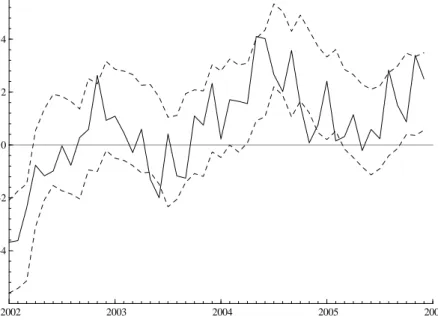
out that using ICI in a bivariate non-parametric approach is more efficient in sign prediction. Moreover, Pesaran and Timmermann (1992) developed a sign predictability test. Using the ICI, we obtain a test statistic of 9.2, which is well above the 95% critical value of a standard normal variable. There is thus a clear evidence of predictive power in ICI for the IPI movements. Last, we compute prediction intervals as presented in section 2.4. We choose 1995-2002 as learning period and compute B=1000 replications of the smoothed bootstrap residuals. To get narrower confidence intervals, we opt for a confidence level 1 - α equal to 70%. The dynamic one-step-ahead confidence intervals are shown in figure 2.
Conclusion
In this paper, we introduce a non-parametric Kernel-based method in order to predict the one-month-ahead manufacturing Euro area IPI using industrial opinion surveys. Moreover, we compute confidence intervals for the predictor based on the re-sampling Bootstrap
methodology. We show that this non-parametric method allows to improve the forecasting performances with respect to more classical techniques. This approach could be fruitfully used to asses the current state of the industrial activity during the 45 days between releases of IPI and opinion surveys.
References
Angelini, E, G. Camba-Mendez, D. Giannone, L. Reichlin and G. Rünstler (2008), Short-term forecasts of Euro area GDP growth, Discussion Paper Series No. 6746, CEPR.
Bengoechea, P., M. Camacho and G. Perez-Quiros (2006), A useful tool for forecasting the Euro area business cycle phases, International Journal of Forecasting, 22, 735-749.
Cao, R. and Vilar-Fernández, J.M. (2007), Nonparametric forecasting in time series. A comparative study, Communications in Statistics / Simulation and Computation, 36, 3043-3057.
Collomb, G. (1984), Propriétés de convergence presque complète du prédicteur à noyau, Zeitschrift für
Wahrseinlichkeitstheorie, 66, 441-460.
Diron, M. (2006), Short-term forecasts of euro area real GDP growth: An assessment of real time performance based on vintage data, Working Paper No. 622, European Central Bank.
Diebold, F.X. and R.S. Mariano (1995), Comparing predictive accuracy, Journal of Business and
Economic Statistics, 13, 253-263.
Ferrara, L. (2007), Point and interval nowcasts of the euro area IPI, Applied Economics Letters, 14, 2, 115-120.
Härdle, W., and Vieu, P. (1992) Kernel regression smoothing of time series, Journal of the Time Series
Analysis, 13, 209-232.
Harvey, D.I., Leybourne, S.J. and P. Newbold (1997), Testing the equality of prediction mean squared errors, International Journal of Forecasting, 13, 281-291.
Matzner-Lober, E., Gannoun, A. and De Gooijer, J.G. (1998), Nonparametric forecasting: Comparison of three kernel-based methods, Theory and Methods, 27 , 1593-1617.
Pesaran, H. and Timmermann, A. (1992), A Simple Nonparametric Test of Predictive Performance,
Journal of Business & Economic Statistics, 10, 4, 561-65.
Sédillot, F., and N. Pain (2005), Indicator models of real GDP growth in the major OECD countries,
OECD Economic Studies, No. 40, 2005/1, 167-217.
Thomakos, D. and Guerard, J. (2004), Naive, ARIMA, nonparametric, transfer function and VAR models: A comparison of forecasting performance, International Journal of Forecasting, vol. 20(1), 53-67.
Table 1. Prediction criteria for the IPI annual growth rate (period 2002-2005) (p,q) MAE RMSE item 1 (2,1) 0.91 1.13 item 2 (3,1) 1.00 1.23 item 3 (2,1) 1.17 1.46 item 4 (2,2) 1.09 1.32 item 5 (3,1) 1.02 1.20 item 6 (3,2) 1.02 1.24 item 7 (2,1) 1.06 1.24 BCI (2,4) 0.97 1.17 ICI (3,2) 0.88 1.09 Naive 1.14 1.38 Univariate NP 3 1.03 1.23 ARMA (3,0) 1.06 1.25
Table 2. Prediction criteria for the IPI annual growth rate (period 2002-2005)
2002 2003 2004 2005
MAE RMSE MAE RMSE MAE RMSE MAE RMSE ICI 0.67 0.90 0.87 1.08 1.10 1.30 0.90 1.08
Naive 0.95 1.15 1.12 1.38 1.25 1.49 1.26 1.50
Univariate NP 0.94 1.17 0.99 1.14 1.30 1.47 0.92 1.15
Table 3. Prediction criteria: Success Ratio (period 2002-2005)
Success Ratio
ICI 0.78
Univariate NP 0.68
Figure 1. IPI annual growth rate (in %) and the non-parametric kernel predictor wit h ICI (2002-2005) 2002 2003 2004 2005 2006 -3 -2 -1 0 1 2 3 4 IPI Prediction
Figure 2. Bootstrapped confidence interval at the 0.70 confidence level (2002-2005)
2002 2003 2004 2005 2006 -4 -2 0 2 4