HAL Id: hal-02946364
https://hal.archives-ouvertes.fr/hal-02946364
Submitted on 7 Oct 2020
HAL is a multi-disciplinary open access
archive for the deposit and dissemination of sci-entific research documents, whether they are pub-lished or not. The documents may come from teaching and research institutions in France or abroad, or from public or private research centers.
L’archive ouverte pluridisciplinaire HAL, est destinée au dépôt et à la diffusion de documents scientifiques de niveau recherche, publiés ou non, émanant des établissements d’enseignement et de recherche français ou étrangers, des laboratoires publics ou privés.
Injection height of biomass burning aerosols as seen
from a spaceborne lidar
Mathieu Labonne, François-Marie Bréon, Frederic Chevallier
To cite this version:
Mathieu Labonne, François-Marie Bréon, Frederic Chevallier. Injection height of biomass burning aerosols as seen from a spaceborne lidar. Geophysical Research Letters, American Geophysical Union, 2007, 34 (11), pp.L11806. �10.1029/2007GL029311�. �hal-02946364�
Injection height of biomass burning aerosols as seen from a spaceborne
lidar
Mathieu Labonne,1 Franc¸ois-Marie Bre´on,1 and Fre´de´ric Chevallier1
Received 10 January 2007; revised 16 March 2007; accepted 27 April 2007; published 5 June 2007.
[1] This paper analyzes new lidar measurements from
space over regions of biomass burning activity. The height of the aerosol layers deduced from the lidar observations is compared to the mixing layer top diagnosed from numerical weather forecasts, to identify whether or not the aerosols are directly injected in the free troposphere. During July and August 2006, the best cases (limited cloudiness, high density of fires) are found over South Africa and Northern Australia. Over these regions, the top of the aerosol layer is close to the mixing layer height, which is a strong indication that the aerosols are injected within the mixing layer. Other tropical areas with biomass burning activity are more difficult to interpret but the valid data support the same conclusion. For higher latitudes regions with biomass burning activity, although several aerosol plumes are identified above the mixing layer, most of the load is within the mixing layer. These observations made over a limited period and set of regions indicate that cases with pyro-convection and/or direct injection to the free troposphere are not frequent. Citation: Labonne, M., F.-M. Bre´on, and F. Chevallier (2007), Injection height of biomass burning aerosols as seen from a spaceborne lidar, Geophys. Res. Lett., 34, L11806, doi:10.1029/2007GL029311.
1. Introduction
[2] Biomass burning is a major contributor of trace gases
and aerosols to the atmosphere, which affects its chemistry, in particular ozone formation. Although some fires have a natural origin, a large fraction of biomass burning results from anthropogenic activities, either for clearing a forest and making place to new agriculture and grazing, or through annual agricultural practices. Over a given region affected by such processes, biomass burning has a very strong annual cycle, with a peak during the dry season. Satellite observations of active fires [e.g., Justice et al., 2002] and burned surfaces have provided useful information on the amount of burning and on its inter-annual variations.
[3] In addition to solid and gaseous material, fires release
considerable amount of heat. The resulting plume possesses some buoyancy that generates strong updrafts above the fire. If the plume kept its initial buoyancy, it would rise to considerable heights in the atmosphere. However, strong turbulence mixes the plume with the surrounding air so that the plume temperature and the buoyancy are reduced. Eventually, the plume reaches a stable layer at which the updraft stops. Because of turbulence and mixing, the fire
products are not entirely injected at this maximum height, but are rather distributed unevenly between the surface and the top height. Note that the updraft may lead to conden-sation within the plume, which releases some latent heat and increases the plume buoyancy [Freitas et al., 2006] and cases with direct injection in the stratosphere have been reported [e.g., Damoah et al., 2006].
[4] After this initial injection phase, the material enters
the general atmospheric circulation. The fraction that is within the boundary layer height is well mixed by diurnal convection. On the other hand, the fraction that reaches the free troposphere is then transported over very long distan-ces. Indeed, the transport in the free troposphere is faster than in the boundary layer and, more importantly, there is less removal of material by scavenging and wet-removal processes. As a consequence, the injection height is a major parameter for a proper understanding and modeling of the atmospheric chemistry. It is also of considerable importance for the interpretation of observations [e.g., Che´din et al., 2005].
[5] This study investigates the initial injection height of
aerosol generated by biomass burning. Deep moist convec-tion and dynamic processes transport some of the material from the boundary layer to the free troposphere, but this requires longer time scales (biomass burning occurs during the dry season so that moist convection is unlikely in the immediate vicinity of the fires). Note that such processes are realistically accounted for in atmospheric circulation models in contrast to injection heights. In this paper, we focus on the initial injection, i.e. we analyze the aerosol distribution in the immediate vicinity of the fires.
[6] For that purpose, we make use of the recently
released data from the Cloud Aerosol Lidar and Infrared Pathfinder Satellite Observations (CALIPSO) spaceborne lidar and analyze the vertical distribution of aerosols in areas that are strongly affected by biomass burning. We assume that the aerosol is a good marker of the fire emissions. Therefore, the aerosol profile provides some information on the injection height. The results are based on a visual analysis and interpretation of several hundred slices of the atmosphere that we extracted from the dataset over regions of intense biomass burning activity, together with statistical analysis of the CALIPSO aerosol products.
2. Data
2.1. MODIS Active Fire
[7] For the identification of the areas that are affected by
biomass burning, we used the Moderate Resolution Imaging Spectroradiometer (MODIS) active fire product [Justice et al., 2002; Giglio et al., 2003]. The fires are identified based on the temperature at wavelength 4mm compared to that at
1
Laboratoire des Sciences du Climat et de l’Environnement, Institut Pierre-Simon Laplace, CEA, CNRS, UVSQ, Gif sur Yvette, France.
Copyright 2007 by the American Geophysical Union. 0094-8276/07/2007GL029311
11mm. Thanks to the very non-linear characteristic of the Planck function, hot fires have a very distinct signature even when they cover a fraction of the MODIS pixel. The active fire product includes a confidence index that was used here with a threshold at 80%.
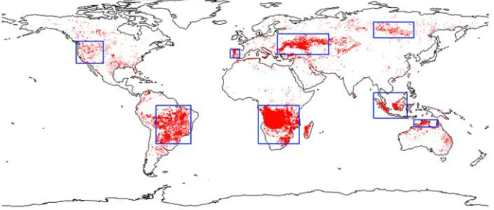
[8] Figure 1 shows the locations of the actives fires
identified from MODIS observations during July and August 2006. A large fraction of the fires are observed over Southern Africa and correspond to burning savanna as studied during the SAFARI2000 field campaign [Privette and Roy, 2005]. Other locations show an intense biomass burning activity and we have selected eight different zones that are representative of tropical, mid-latitude and high-latitude fires (see Table 1).
2.2. CALIPSO
[9] The CALIPSO satellite is a collaborative effort
between the US and the French space agencies, respectively NASA and Centre National d’E´ tudes Spatiales (CNES). It was launched on April 28, 2006 and carries a two-wavelength lidar at 532 and 1064 nm. As a first step, we have used the level 1 data, i.e. the attenuated backscatter. A visual analysis of the two channels, together with their ratio, permits an easy identification of the aerosols and cloud layers (see an example in Figure 2). In this paper, we focus on the CALIPSO measurements acquired in July and August 2006, first because they were available at the beginning of this study, and also because this period includes the peak of the biomass burning season both in
the tropics (South Africa) but also over mid and high latitude of the Northern hemisphere.
[10] Note that the lidar backscatter data are rather noisy
and require significant averaging for a proper identification of the aerosol layers. The amount of noise is a function of the reflected solar flux, so that daytime measurements and scenes with a high albedo are the most affected. We have adapted the level of smoothing to each case. Aerosol layers appear rather smooth with a large spatial extension so that little information is lost in the spatial smoothing.
[11] For a statistical analysis of the results, we have
attempted to use the CALIPSO aerosol layer product. This product provides a description of the aerosol layers, including their top heights and bottoms, identified from the level-1 data. However, the first and current release of this product shows many errors where clouds are identified as aerosols and vice-versa. As a consequence, much caution is necessary in its use. As an attempt to reject layers erroneously identified as aerosols (in particular below cloud decks), we have set a threshold to the integrated atmospheric backscatter at 0.02 sr 1. Profiles with larger values are not used for the statistical analysis. Although efficient, this simple procedure does not eliminate all errors in the level-2 product and caution is required in the analysis these data.
2.3. ECMWF Mixing Layer Height
[12] As explained above, the main objective of this paper
is to analyze the height of the aerosol layer in relation to that of the mixing layer. We have therefore used the data from Figure 1. Global distributions of active fires as seen by the MODIS instrument during July and August of 2006. The boxes indicate the various areas that are analyzed in detail in this paper.
Table 1. Summary of Aerosol Layer Top Height and Boundary Layer Height in the Eight Analyzed Regionsa
Case Names Dates
Number of Cases
Range of Top Height of the Aerosol Layers
ECMWF Boundary Layer
Typical Values A South Africa July + August 130 3 to 4.5 kms 3 to 4.5 kms B South America July + August 137 1.5 to 3.5 kms 1.5 to 3.5 kms C North of Australia August 42 2 to 2.5 2 to 2.5 D Indonesia August 66 2 to 2.5 kms with 2 peaks at 3 kms 1.5 to 2.5 kms
E Portugal August 20 1,5 to 5 kms 1,5 to 4.5 kms
F Western USA July + August 107 4 to 7 kms 4 to 7 kms G Eastern Europe July + August 178 Large range: 1.5 km to
6 kms
Large range: 1.5 km to 4.5
H Siberia July 70 2 to 4 kms 2 to 3.5 kms
aThe number of cases indicates the total number of CALIPSO passes, some of them are not useful for our analysis because of the cloud cover. The top
height of the aerosol layer that can be identified from a visual analysis of the data in region of active fires gives an estimate of the maximum injection height.
L11806 LABONNE ET AL.: INJECTION HEIGHT AS SEEN FROM SPACE L11806
the European Centre for Medium-range Weather Forecast (ECMWF) that provides a diagnostic of the boundary layer height. This product is available with a 3-hourly and 25 km resolution.
[13] The parameterization of the mixed layer (and
entrainment) already uses a model level index as boundary layer height, but in order to get a continuous field, also in neutral and stable situations, the parcel lifting method (or bulk Richardson method) is used as a diagnostic, indepen-dent of the turbulence parameterization (see the model documentation at http://www.ecmwf.int/research/ifsdocs/ CY28r1/Physics/Physics-04-09.html#wp972354). The three-hourly fields show a strong diurnal cycle (low values at night). Since we are interested in the layer that is mixed during the diurnal convection, the largest value of the day is used as a proxy of the mixing layer height. In the following, we refer to this daily maximum as the mixing layer.
3. Case Study
[14] Figure 2 illustrates one of the many cases that we
have analyzed. The image is based on the attenuated backscatter at wavelength 532 nm, although our analysis uses the other channel as well. Biomass burning aerosols have a much larger response at 532 nm than in the longer wavelength channel while clouds and coarse mode aerosols show similar responses. This provides an easy method to distinguish fine aerosols and cloud layers. The CALIPSO track passes right over an area with many active fires (see Figure 2). It is therefore reasonable to assume that the thick plume observed over this area is mostly generated by active fires of the same day. Figure 2 indicates that the plume is contained within the mixing layer which top height is around 4.5 km according to ECMWF. Figure 2 (right) corresponds to the Southern part of the track, which is over the ocean. Over this area, the mixing layer is much thinner (1 – 2 km) and capped by stratocumulus clouds. The
bio-mass burning plume is transported over the cloud deck, well above the mixing layer but as a consequence of remote transport, not of direct injection. On the left side of the image, which corresponds to the Northern part of the track, high clouds are present and limit the observation capabili-ties. Nevertheless, an aerosol plume can be observed around 4 km over a region with a lower mixing layer and where no active fires are observed. Therefore, this aerosol layer also results from atmospheric transport.
[15] For this particular case, there is therefore strong
indication that the initial injection of the biomass burning aerosol is within the boundary layer, while atmospheric flow transports the aerosol in areas where the boundary layer is much lower.
4. Global Analysis
[16] We have analyzed several hundred cases such as
those shown in Figure 2. In the following we discuss the findings for each of the eight regions that were selected based on Figure 1. Cases A – D correspond to tropical areas, whereas cases E – H are at mid and high latitudes. Table 1 provides a summary of the injection height in relation to the mixing layer depth.
4.1. Case A: South Africa
[17] The observation of aerosol layers over South Africa
with the CALIPSO lidar is rather easy with very little interference by clouds. A large area is affected by the fires (see Figure 1) and they are persistent during July and August. Over this area, ECMWF indicates a mixing layer height of 3 to 4.5 km. There is a surprisingly good correspondence between the ECMWF diagnostic and the top of the aerosol layer, an example of which is shown in Figure 2. For most cases, the top of the aerosol layer is very close (i.e. within 500 meters) to the boundary layer given by Figure 2. (left) An example of lidar backscatter profile at 532 nm together with ECMWF boundary layer height (yellow line), as analyzed in this paper, and the location of the corresponding CALIPSO subtrack. On the lidar profile, the black line shows the surface level and the logarithm of the attenuated backscatter is shown on a rainbow color scale from purple (0.001 km 1sr 1) to red (0.1 km 1sr 1). The spike around 20°S is the Brandberg massif in Namibia. (right) On the map, the color of the dots indicates the temporal difference between the fire and the lidar observation: red, same day; green, previous day; blue, 2 days before. The wind speed and direction retrieved from ECMWF are represented with the orange arrows. The length of the arrow corresponds to the atmospheric transport within half a day at 850 hPa (around 1.5 km above sea level).
the ECMWF model, especially when the satellite subtrack is right above fires.
[18] For a quantitative analysis, we use the CALIPSO
aerosol layer product. Figure 3 shows the histogram of the difference between the upper aerosol layer top and the ECMWF mixing layer height. Such a result should be interpreted with caution since the aerosol layer product still shows many errors. Nevertheless Figure 3 confirms that there is a high coherence between the mixing layer and the aerosol layer heights. Indeed, they agree within 500 m in 75% of the cases. Besides, visual analysis confirms that most of the other cases result from erroneous aerosol identification. In Figure 3, we distinguish cases that are ‘‘close’’ and ‘‘far’’ from active fires. Cases where the aerosol layer is well above the mixing layer top tend to be ‘‘far’’ from the sources. This observation confirms that, in this region, the presence of aerosol above the mixing layer is a result of remote atmospheric transport rather than of direct injection.
4.2. Case B: South America
[19] South America is another area with intense biomass
burning during July and August. On the other hand, cloudiness is much higher than it is over South Africa at the same period, which makes the analysis of the lidar data more difficult. As for South Africa, there is a surprisingly good correspondence between the ECMWF diagnostic and the top of aerosol layers. The histogram analysis (similar to Figure 3, not shown) shows a high coherence but is less conclusive than for case A as a result of smaller sample (higher cloudiness and fewer active fires). Although the mixing layer depth is somewhat smaller than over South Africa, the analysis of the valid cases supports the conclusions made for case A.
4.3. Case C: Australia
[20] As for South Africa, the observation is easy thanks to
a very low cloudiness above North Australia in August. There is a small area with a high density of biomass burning activity that generates aerosol layers easily identified on the
lidar products. The correspondence between the ECMWF mixing layer and the aerosol layer top is excellent. Most cases show a mixing layer thickness of about 2 km. Among the cases analyzed for this paper, only one showed a much higher thickness (up to 3.5 km) as identified by both the lidar image and the ECMWF. The histogram (not shown) confirms these findings with 80% of the aerosol layer tops in the 500 m just below the ECMWF diagnostic.
4.4. Case D: Indonesia
[21] MODIS data indicate an intense biomass burning
activity over Indonesia, in particular during August. Cloud-iness is high over this area, which makes the analysis more difficult than over the other regions analyzed above. The quantitative analysis requires the rejection of many cases that are corrupted as a result of the erroneous identification of cloud layers as aerosols. Valid cases support the conclu-sion that biomass burning plumes are injected within the mixing layer as identified by the ECMWF.
4.5. Case E: Portugal
[22] Portugal experienced a series of devastating fires
during the first half of August 2006, which location is clearly identified by MODIS. This region constitutes an interesting case study because the area affected by the fires is rather small in comparison to the other cases analyzed here. On the other hand, few CALIPSO passes are exactly over the affected area. These cases indicate that the aerosol plume reaches a few km (up to 5), which is consistent with the mixing layer depth over the Iberic Peninsula. Some cases show the plume transported over the Atlantic Ocean, in which case it is well above the mixing layer. There are too few cases to derive meaningful histogram and statistics. 4.6. Case F: Western USA
[23] There were many fires over the western part of the
USA during the summer of 2006 as identified by MODIS data (see Figure 1) although the density is much smaller than for the other cases analyzed here. The affected area is mostly mountainous and ECMWF diagnoses a mixing layer top around 5 km above sea level. The lidar observations clearly show that most of the aerosol is contained within the ECMWF mixing layer. The active fire density is much smaller than that over the tropical areas analyzed above so that individual plumes are observed rather than a large-scale aerosol layer. There are a few cases where the lidar track is directly above well-identified active fires. For such cases, the aerosol plume is within the mixing layer. Other cases with aerosol layers above the mixing layer top cannot be related to active fires so that they may result from atmo-spheric transport.
4.7. Case G: Eastern Europe
[24] Many fires are reported by MODIS over Eastern
Europe during the period of interest (see Figure 1). These fires occurred mostly after July 15th. Aerosol layers are clearly depicted by the lidar over the same area at variable altitudes up to 6 km. Although the aerosols layers are often contained within the mixing layer, there are also a large number of cases where they extend well above the ECMWF diagnosed top height. Such cases may result from direct injection in the free troposphere as reported for biomass burning events in mid and high latitude [Fromm et al., Figure 3. Statistical analysis of the difference in km
between the ECMWF mixing layer height and the top height of the aerosol layer identified in the CALIPSO standard product for the area A (South Africa) for July and August (CALIPSO minus ECMWF). Both the histogram and the cumulative histogram are shown for locations within 80 km of a fire (plain lines) and those further than 140 km from a fire (dashed lines).
L11806 LABONNE ET AL.: INJECTION HEIGHT AS SEEN FROM SPACE L11806
1998; Jost et al., 2004]. However, synoptic transport, including moist convection, cannot be ruled out and a further investigation would require atmospheric transport modeling.
4.8. Case H: Siberia
[25] Many fires were detected by MODIS over Siberia
during July and August 2006. Unfortunately, the cloudiness is rather high which makes difficult the analysis of the lidar data. There are a few well identified aerosol layers however. The bulk of the aerosol load is clearly within the mixing layer. There are a few cases with significant load above the ECMWF diagnosed top level. On the other hand, we were not able to unambiguously relate those layers to active fires. Thus, these aerosol layers in the free troposphere may result from atmospheric transport rather than direct injection.
5. Discussion and Conclusions
[26] One potential bias in our procedure results from the
higher quality of the nighttime lidar data while biomass burning is mostly daytime, in particular when it results from agricultural practices. Daytime data are considerably noisier than nighttime’s due to the solar contribution to the mea-surement. However, spatial averaging of the data provides images of good quality that are suitable to identify clouds and aerosol layers. Our analysis of such images did not identify meaningful difference in the structure of the aerosol layers between daytime and nighttime.
[27] For the analysis of the aerosol height in relation to
the mixing layer thickness, the best cases were found over South Africa and Australia. Over these regions, a high density of fires and the absence of clouds made the analysis much easier than over other areas. The data strongly support the conclusions that biomass burning plumes are injected within the mixing layer, the depth of which is remarkably diagnosed by the ECMWF short-range forecast. The aerosol plume may then be transported by the atmospheric flow over regions with a lower mixing layer depth, i.e. to the free troposphere. The other tropical areas are affected by cloudiness, which makes the analysis more difficult. Although no case with direct injection to the free tropo-sphere has been identified, it cannot be ruled out.
[28] Over mid and high-latitudes areas, there are several
reports of biomass burning plumes injected well above the mixing layer, up to the upper-troposphere or even the stratosphere. Although the CALIPSO lidar data do show some aerosol layers above the mixing layers, none of the analyzed cases could be unambiguously related to an active
fire, so that the presence of aerosol in the free troposphere might be the result of atmospheric transport rather than direct injection. The few cases where the source fire could be identified showed a plume within the mixing layer (as diagnosed by ECMWF). These results indicate that, although cases with direct injection to the free troposphere have been reported, most biomass burning plumes are initially limited to the mixing layer. Note that this conclu-sion is also supported by an analysis of MISR aerosol heights [Mazzoni et al., 2007]. The fact that the biomass burning plumes are hardly injected above the mixing layer should facilitate their inclusion in general circulation models, even though some specific cases or applications may neces-sitate elaborate parameterizations.
[29] Acknowledgments. We thank NASA and CNES for making the CALIPSO data available to the scientific community and the ICARE thematic center for its assistance. This study was partly funded by the European Union under project GEMS.
References
Che´din, A., S. Serrar, N. A. Scott, C. Pierangelo, and P. Ciais (2005), Impact of tropical biomass burning emissions on the diurnal cycle of upper tropospheric CO2retrieved from NOAA 10 satellite observations,
J. Geophys. Res., 110, D11309, doi:10.1029/2004JD005540.
Damoah, R., N. Spichtinger, R. Servranckx, M. Fromm, E. W. Eloranta, I. A. Razenkov, P. James, M. Shulski, C. Forster, and A. Stohl (2006), A case study of pyro-convection using transport model and remote sensing data, Atmos. Chem. Phys., 6, 173 – 185.
Freitas, S. R., et al. (2006), Including the sub-grid scale plume rise of vegetation fires in low resolution atmospheric transport models, Atmos. Chem. Phys. Discuss., 6, 11,521 – 11,559.
Fromm, M., J. Alfred, K. Hoppel, J. Hornstein, R. Bevilacqua, E. Shettle, R. Servranckx, Z. Li, and B. Stocks (1998), Observations of boreal forest fire smoke in the stratosphere by POAM III, SAGE II, and lidar in 1998, Geophys. Res. Lett., 27, 1407 – 1410.
Giglio, L., J. Descloitres, C. O. Justice, and Y. J. Kaufman (2003), An enhanced contextual fire detection algorithm for MODIS, Remote Sens. Environ., 87, 273 – 282, doi:10.1016/S0034-4257 (03)00184-6. Jost, H.-J., et al. (2004), In-situ observations of mid-latitude forest fire
plumes deep in the stratosphere, Geophys. Res. Lett., 31, L11101, doi:10.1029/2003GL019253.
Justice, C. O., L. Giglio, S. Korontzi, J. Owens, J. T. Morisette, D. Roy, J. Descloitres, S. Alleaume, F. Petitcolin, and Y. Kaufman (2002), The MODIS fire products, Remote Sens. Environ., 83, 244 – 262. Mazzoni, D., J. A. Logan, D. Diner, R. Kahn, L. Tong, and Q. Li (2007), A
data-mining approach to associating MISR smoke plume heights with MODIS fire measurements, Remote Sens. Environ., 107, 138 – 148. Privette, J. L., and D. P. Roy (2005), Southern Africa as a remote sensing
test bed: The SAFARI 2000 special issue overview, Int. J. Remote Sens., 26(19), 4141 – 4158.
F.-M. Bre´on, F. Chevallier, and M. Labonne, Laboratoire des Sciences du Climat et de l’Environnement, Institut Pierre-Simon Laplace, CEA, CNRS, UVSQ, F-91191 Gif sur Yvette, France. (mathieu.labonne@cea.fr)