A BGK-type model for inelastic Boltzmann equations with internal energy.
Texte intégral
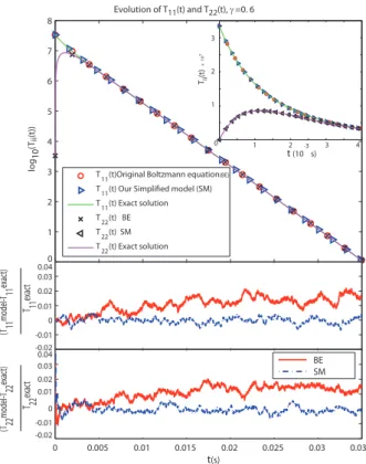
Figure


Documents relatifs
This paper is devoted to the proof of the convergence of the solution of the Boltzmann equation, for a degenerate semiconductor and with an arbitrary band structure, towards
Finally, we would like to mention that there are also some interesting results on the uniqueness for the spatially homogeneous Boltzmann equation, for example, for the Maxweillian
well suited to the mild solution concept used for soft forces, and this paper includes the first general existence proof for the nonlinear stationary
We prove an inequality on the Kantorovich-Rubinstein distance – which can be seen as a particular case of a Wasserstein metric– between two solutions of the spatially
For the Landau equation, lower and upper bounds for the solution have been obtained in [21] using integration by parts techniques based on the classical Malliavin calculus..
Navier-Stokes equations; Euler equations; Boltzmann equation; Fluid dynamic limit; Inviscid limit; Slip coefficient; Maxwell’s accommo- dation boundary condition;
(This is easily seen for instance on formula (1.2) in the special case of the radiative transfer equation with isotropic scattering.) At variance with the usual diffusion
However, the study of the non-linear Boltzmann equation for soft potentials without cut-off [ 20 ], and in particular the spectral analysis its linearised version (see for instance [
