Contextual Enhancement Of Satellite Images

République Algérienne Démocratique et Populaire

Ministère de l'Enseignement Supérieur et de la Recherche Scientifique Université de Batna

Faculté des Sciences de l'Ingénieur Département d'Electronique

Thèse

Contextual Enhancement

Of Satellite Images

En vue de l'obtention du diplôme de

Docteur d'état en électronique

Option: contrôle et traitement de signal

Par

SOUAD BENABDELKADER

Jury

Président N. Bouguechal Professeur (Université de Batna) Rapporteur M. Boulemden Professeur (Université de Batna) Examinateur D. Benatia Professeur (Université de Batna)

Examinateur M. Benyoucef Maître de conférence (Université de Batna) Examinateur F. Hachouf Maître de conférence (Université de Constantine) Examinateur S. Chikhi Maître de conférence (Université de Constantine)

Acknowledgments

I

t has been a long time since the last acknowledgments.

I would like to take this opportunity to express my thanks to Professor Mohammed Boulemden for his patience and encouragement that have been a true strength to complete this study.

I would like to thank Professor Noureddine Bouguechal from the Electronics Department at the University of Batna to preside at my maintaining thesis. Thank you very much to all the examining board members for their interest in my work namely, Dr. Fella Hachouf from the Electronics Department at the University of Constantine, Dr. Salim Chikhi from the Department of Computer Science of the University at Constantine, Prof. Djamel Benatia and Dr. Moussa Benyoucef from the Electronics Department at the University of Batna. I am deeply grateful for helping me to be finally in time before the dead line of December 31th.

I am very grateful to Dr. Farid Melgani with whom the essential of this work has been achieved. I would like to thank him for introducing me to the image restoration field and his constant supervision during the year I spent at the Dipartimento di Informatica at the University of Trento in Italy.

Thank you very much to my friends Lemia, and Samira for their constant support.

I am also very grateful for the assistance given to me by my friends and colleagues Dr. Djamel Benatia, Dr. Ramdane Mahammdi and Dr. Tarek Fortaki.

Dedications

W

ednesday, December 18, 2008, was the day of my doctorate thesis discussion. My parents could not be physically present because my father was ill with bronchitis since two weeks.

A

t that day, I left early with the precious prayers of my mother and my youngest sister

Roukia. I could not see my father before leaving. He was in pain and I did not want to worry

him.

W

hen coming home in the afternoon, my father was up out of bed for the first time since several days. He looked tired but so glad. We celebrated the event in family and took photos, the last we had with my father alive.

T

hree weeks after, exactly in Tuesday, January 6, 2009, my father died. Now that I think of it, I thank ALLAH day and night to have allowed me finishing this thesis before my father departs this life for ever.

T

his thesis is dedicated to the memory of my father, Si Larbi El-Khroubi. An adherent of the revolutionary agitation since his childhood. A great Hero of November, 1st, 1954. A man who had a partiality for his religion and nation; he went in Palestine in 1948, but the British army caught him with his four companions at the frontier between Libya and Egypt. The French authorities put them in prison for three months. A man who lived and died with honor and honesty. A model citizen. A model of all virtues. A father who taught us the love of Islam, family and country. A father who taught us how to read a newspaper at seven. A friend of his daughters. A Great Father, The Best.

T

his thesis is dedicated to my mother with all my love and respect. She corrected my compositions in the primary school, stood awake with me in the secondary school and university, and was longing for me to get the doctorate degree.

Abstract

I

mages are the main sources of information in many applications. However, the images obtained from various imaging systems are subject to degradations and loss of information. In the field of remote sensing, cloud obscuration presents a major impediment to the effective use of passive remotely sensed imagery. Cloud occurrence distorts or completely obscures the spectral response of land covers, which contributes to difficulties in understanding scene content. Therefore, a cloud removal task is needed as the primary important step to recover the missing measurements. Recently, cloud removal has been addressed as an image reconstruction/restoration issue, in which it is aimed at recovering an original scene from degraded or missing observation.

As a first application for remote sensing, we propose three general methods for post-restoration of cloud contaminated areas in multispectral multitemporal remote sensing images. Spatial, temporal and spectral information are incorporated in the post-restoration processes to analyze which is more suited to improve the restoration quality, depending on the contamination scenario. Experiments have shown that higher accuracies are obtained with the use of mutual spatio-spectral and temporal information.

Second, we address the problem of contrast enhacement for remote sensing application. At this purpose, two variational perspectives to bright preserving contrast enhancement scheme have been proposed. The methods can be viewed as refinements of histogram equalization, which use both local and global information to remap the image gray levels. The brightness preserving constraint is implicitly expressed with the use of a fuzzy 2-partition thresholding process to extract object regions from their background on the basis of the similarity of brightness of image objects.

The first method models the spatial relationships between neighboring pixels with a second order derivative metric which provides a local measure of spatial activity within the data. The second method uses a contextual spatial histogram to describe the gray level distribution in a predefined neighborhood system over a predefined area in the image.

Experiments have shown that the proposed methods increase the brightness preservation and yield a more natural enhancement. They are able to amplify edge contrast without explicitly detecting edge pixels.

Résumé

L

'être humain dépend à 99% de sa vision pour récolter des information sur le monde qui l'entoure. Il est donc naturel que l'imagerie numérique ait pris une importance considérable. Néanmoins, historiquement parlant, les potentialités du traitement numérique des images pour

le transfert et l’amélioration des images sont apparues avec le développement des grands

ordinateurs et surtout avec les nécessités des programmes de recherche spatiale. Puis est venue l'ère de l’explosion des applications dans tous les domaines....

L'imagerie numérique est limitée par les dégradations, généralement désignées sous le terme de bruit d'image, dues aux bruits inhérents aux dispositifs d'acquisition (caméra,

amplificateurs, quantification, …). L'élimination du bruit et le recouvrement de l'information

perdue ou cachée constituent donc une étape cruciale dans le traitement d'image.

D'un autre côté, les images acquises dans des conditions d'éclairage extrêmes; lumière trop faible ou trop puissante ainsi que les images issues de capteurs dont la dynamique est trop réduite sont peu contrastées, ce qui gêne sérieusement les opérations de reconnaissance, d'analyse et d'interprétation. Les méthodes de manipulation d'histogramme sont à l'origine des techniques d'amélioration du contraste, en particulier l'égalisation d'histogramme en raison de sa simplicité et des informations pertinentes à l'amélioration fournies par l'histogramme de l'image.

Il est important de noter que la restauration constitue une opération d'amélioration basée sur un modèle mathématique de la dégradation, alors que l'amélioration du contraste ne prend en considération aucun modèle de bruit, et est par conséquent laissée aux soins de l'observateur pour juger de la qualité de l'amélioration.

Le travail présenté dans cette thèse concerne à la fois restauration et amélioration du contraste appliquées au domaine de la télédétection satellitaire.

La thèse est composée de quatre chapitres.

Le premier chapitre introduit l'état de l'art des méthodes de restauration tout en présentant les critères quantitatifs standard de la qualité de restauration en plus d'un aperçu sur la littérature des méthodes de restauration.

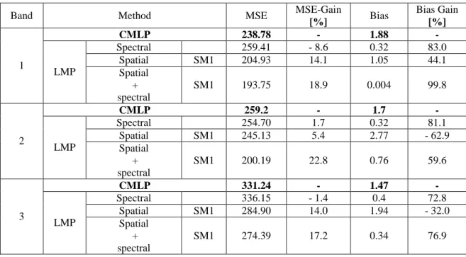
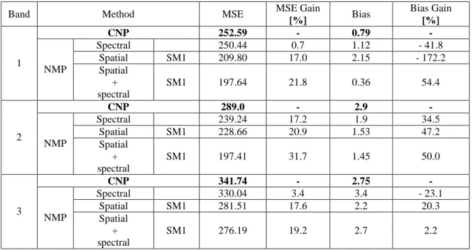
Le deuxième chapitre aborde la restauration du point de vue d'une post-reconstruction de zones contaminées par les nuages dans une séquence d'images multispectrales multitemporelles. L'objectif visé dans ce chapitre est d'améliorer la qualité de restauration obtenue par deux méthodes générales de restauration développées récemment, en l'occurrence la technique dite Contextual Multiple Linear Prediction (CMLP) et celle appelée Contextual Nonlinear Prediction (CNP). Une post-reconstruction est alors effectuée en utilisant conjointement l'information spatiale, spectrale et temporelle. Trois méthodes en guise de solution ont été proposées, en l'occurrence la prédiction multimodale, la prédiction de l'erreur résiduelle issue d'un estimateur et enfin la post-reconstruction spatio-spectrale. La génération d'une Map d'erreur est utilisée comme critère d'évaluation supplémentaire de la qualité de restauration. Les résultats de la simulation ont été présentés à la fin du chapitre.

Le troisième chapitre présente les bases théoriques générales des techniques de modification d'histogramme. Les techniques de transformation ponctuelles sont considérées, en particulier l'égalisation et la spécification d'histogramme qui sont décrites en détail et par l'exemple pour la première. Trois critères de uantitification de la qualité d'amélioration sont présentés et le chapitre s'achève par un aperçu sur la littérature concernant les méthodes d'égalisation d'histogramme.

Le quatrième chapitre concerne l'amélioration du contraste d'images de télédétection satellitaire en utilisant l'égalisation d'histogramme. Deux méthodes sont proposées, chacune se basant sur le seuillage d'une 2-partition floue pour satisfaire au critère de préservation de la luminosité des pixels. L'incorporation de l'information spatiale est exprimée dans la première méthode par le calcul des gradients du second ordre. Dans la deuxième méthode, le modèle spatial est exprimé par un histogramme bi-dimensioonel représentant la distribution spatiale conjointe des niveaux de gris dans un voisinage prédéterminé. Cet histogramme est calculée sur une zone prédéfinie de l'image et est utilisé par la suite pour le calcul de la densité de probabilité cumulative de l'image entière. Finalement, les résultats de la simulation sont présentés à la fin du chapitre.

Contents

INTRODUCTION 1

1. DIGITALIMAGERESTORATION 3

1.1 INTRODUCTION 3

1.2 IMAGEDEGRADATIONMODEL 4

1.3 MEASURE OFIMAGERESTORATIONQUALITY 5

1.3.1 Standard Metrics 5

1.3.2 Accuracy of the Measure 6

1.3.3 Precision of the Measure 6

1.3.4 Meaning of Measurement 6

1.4 LITERATURESURVEY 7

1.4.1 Classical Image Restoration Techniques 7

1.4.2 New Image Restoration Techniques 10

1.5 SUMMARY 12

2. CONTEXTUALPOST-RECONSTRUCTION OFCLOUD-CONTAMINATEDIMAGES 13

2.1 INTRODUCTION 13

2.2 CLOUDREMOVALTECHNIQUES 14

2.3 Problem FORMULATION 17

2.4 PROPOSEDSOLUTIONS 17

2.4.1 Spectral Information Source 18

2.4.2 SPATIAL Information Source 18

2.5 MULTIMODALPREDICTOR 18

2.5.1 Spectral Information 18

2.5.2 Spatial Information 19

2.5.3 Prediction Function 19

2.6.1 Sequential Residual-Based Prediction (SRBP) 21 2.6.2 PARALLEL Residual-Based Prediction (PRBP) 23

2.7 CONTEXTUALSPATIO-SPECTRALPOST-RECONSTRUCTION 24

2.7.1 Description of the Method 24

2.7.2 Spectral Information 25

2.7.3 Spatial Information 25

2.7.4 Prediction Function 26

2.7.5 Error Map Generation 26

2.7.6 ALGORITHMIC Description 27

2.8 EXPERIMENTALRESULTS 28

2.8.1 Data Set Description and Experiment Design 28

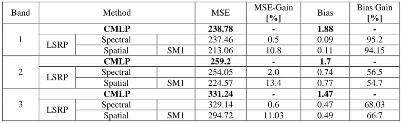
2.8.2 Previous Results 29

2.8.3 Multimodal Prediction Simulations 33

2.8.4 Residual-Based Prediction Simulations 37

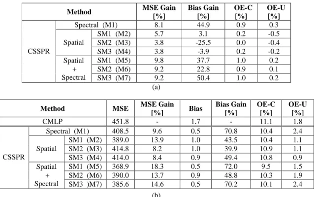
2.8.5 CSSPR Simulations 43 2.9 Summary 49 3. HISTOGRAMMODIFICATION 50 3.1 INTRODUCTION 50 3.2 HISTOGRAMMODIFICATION 51 3.2.1 Contrast of an Image 51 3.2.2 Image Transformation 51 3.2.3 Histogram Processing 51 3.3 QUALITYMEASURES 56

3.3.1 Absolute Mean Brightness Error 56

3.3.2 Contrast –Per-Pixel 55

3.3.3 Image Distortion 56

3.4 LITERATURESURVEY 56

3.5 SUMMARY 58

4. CONTRASTENHANCEMENTOFSATELLITEIMAGESBASEDSPATIALCONTEXT59

4.1 INTRODUCTION 59

4.2 CONTRASTENHANCEMENTBASEDTHRESHOLDING 59

4.2.1 Brightness Preserving Bi-Histogram Equalization 60 4.2.2 Dualistic Sub-Image Histogram Equalization 62

4.2.3 Fuzzy 2-Partition Thresholding 62 4.2.4 Fuzzy 2-Partition Thresholding for Local Contrast Enhancement 68 4.3 CONTEXTUALSPATIALHISTOGRAMFORCONTRASTENHANCEMENT 70

4.3.1 Contextual Spatial Neighborhood 70

4.3.2 Contextual Spatial Histogram 70

4.3.3 Contextual Cumulative Density Function 70

4.3.4 Algorithm 71

4.4 EXPERIMENTALRESULTS 71

4.4.1 Local Contrast Enhancement Based Thresholding Simulations 71 4.4.2 Contextual Spatial Histogram for Contrast Enhancement Results 72

4.5 SUMMARY 72

CONCLUSION 88

List of Figures

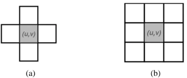
Figure 2.1 Neighborhoods system 18

Figure 2.2 Block diagram of the SRBP system 22 Figure 2.3 Block diagram of the PRBP system 24 Figure 2.4 Block scheme of the whole contextual reconstruction process 25 Figure 2.5 Original sub-images in the Visible range used in the simulations 29 Figure 2.6 Original sub-images in the Infra-Red range used in the simulations 30 Figure 2.7 Masks adopted to simulate different cloud contaminations 30

Figure 2.8 CMLP reconstruction results 31

Figure 2.9 Linear multimodal prediction reconstruction results of channel 1 34 Figure 2.10 Linear multimodal prediction reconstruction results of channel 2 35 Figure 2.11 Linear multimodal prediction reconstruction results of channel 3 35 Figure 2.12 Nonlinear multimodal prediction reconstruction results of channel 1 36 Figure 2.13 Nonlinear multimodal prediction reconstruction results of channel 2 36 Figure 2.14 Nonlinear multimodal prediction reconstruction results of channel 3 37 Figure 2.15 Linear sequential residual-based prediction results of channel 1 40 Figure 2.16 Linear sequential residual-based prediction results of channel 2 40 Figure 2.17 Linear sequential residual-based prediction results of channel 3 41 Figure 2.18 Linear parallel residual-based prediction results of channel 1 41 Figure 2.19 Linear parallel residual-based prediction results of channel 2 42 Figure 2.20 Linear parallel residual-based prediction results of channel 42 Figure 2.21 Reconstruction results with the CSSPR method 45 Figure 2.22 Color composite result with the CSSPR method 46 Figure 2.23 Plotting graphs inside the contaminated area 47 Figure 2.24 Multichannel classification maps obtained by the K-means algorithm 48 Figure 2.25 Reconstruction L2-norm error maps 49 Figure 3.1 Examples of some point processing transformations 52

Figure 3.3 Histogram equalization example 54 Figure 3.4 Illustration of some histogram equalization examples 55

Figure 4.1 Fuzzy membership function 64

Figure 4.2 Contextual spatial neighborhood system 70

Figure 4.3 Two level thresholding results of channel 1 73 Figure 4.4 Two level thresholding results of channel 2 73 Figure 4.5 Two level thresholding results of channel 3 74 Figure 4.6 Two level thresholding results of channel 4 74 Figure 4.7 Two level thresholding results of channel 5 75 Figure 4.8 Two level thresholding results of channel 7 75 Figure 4.9 Local contrast enhancement-based thresholding results of channel 1 77 Figure 4.10 Local contrast enhancement-based thresholding results of channel 2 78 Figure 4.11 Local contrast enhancement-based thresholding results of channel 3 79 Figure 4.12 Local contrast enhancement-based thresholding results of channel 4 80 Figure 4.13 Local contrast enhancement-based thresholding results of channel 5 81 Figure 4.14 Local contrast enhancement-based thresholding results of channel 7 82 Figure 4.15 Masks adopted to simulate different area locations 82 Figure 4.16 Contextual spatial contrast enhancement results of channel 1: Area C outside

the mask 84

Figure 4.17 Contextual spatial contrast enhancement results of channel 4: Area C outside

the mask 85

Figure 4.18 Contextual spatial contrast enhancement results of channel 1: Area C inside

the mask 86

Figure 4.19 Contextual spatial contrast enhancement results of channel 1: Area C inside

List of Tables

Table 2.1 Quantitative results obtained by the linear multimodal prediction 33 Table 2.2 Quantitative results obtained by the non linear multimodal prediction 34 Table 2.3 Quantitative results obtained by the linear sequential residual predictor 38 Table 2.4 Quantitative results obtained by the non linear sequential residual predictor 38 Table 2.5 Quantitative results obtained by the linear parallel residual predictor 39 Table 2.6 Quantitative results obtained by the non linear parallel residual predictor 39 Table 2.7 Quantitative results obtained by the CSSPR method 44 Table 3.1 Histogram equalization procedure 54 Table 4.1 Quantitative results obtained by the local contrast enhancement based fuzzy

2-partition thresholding scheme 76

Table 4.2 Quantitative results obtained by the contrast enhancement based-contextual spatial histogram scheme: Area C outside the mask 83 Table 4.3 Quantitative results obtained by the contrast enhancement based-contextual spatial histogram scheme: Area C inside the mask 83

INTRODUCTION

T

he main part of the information received by a human is visual. Receiving and using visual information is referred to as sight perception or understanding. When a computer receives and uses visual information, we call this computer image processing and recognition. The modern advancement in this area is mainly due to the recent availability of image scanning and display hardware at a reasonable cost, the relatively free use of computers and the popularization of numerous computer processing techniques.

One of the major problems that have evolved in computer image processing was the

degradation of the images in use. Images obtained from various imaging systems are subject

to degradations and loss of information which could be devastating in many applications. The two main limitations in image accuracy are blur and noise. As a result, it was not long before the work on using computer techniques for retrieving meaningful information from degraded images began, what is today known as digital image restoration.

Images are captured in an excessively bright or dark environment in a number of different situations (e.g., pictures taken at night or against the sun rays). As a result, the images are low contrasted, i.e. too dark or too bright, and inappropriate for visual inspection and human interpretation and analysis. Improving the visual quality and enhancing the contrast of images constitutes one of the major issues in image processing. Histogram modification, and in particular histogram equalization is one of the basic and most useful operations in image processing. It has been recognized as the ancestor of plentiful contrast enhancement algorithms [1].

Contrast enhancement and restoration techniques are designed to improve the quality of an image as perceived by a human for a specific application. Image restoration is distinct from contrast enhancement techniques, which are designed to manipulate a degraded image in order to reveal subtle details and produce results more pleasing to an observer, without making use of any particular degradation models. Image restoration is applied to the restoration of a known distortion for which an objective criterion can be applied.

Remote sensing images typically contain an enormous amount of information. From the field of computer vision, enhancement procedures among other techniques determine one possibility to extract such information. The aim of the study at hand is to apply some developed algorithms as means for spatial information extraction.

The present thesis may be divided into two parts. The first deals with a contextual post-restoration technique of cloud-contaminated areas in multispectral multitemporel remote sensing images. Spatial, temporal and spectral information are incorporated in the post-restoration process to analyze which is more suited to improve the post-restoration quality. The second part concerns the contrast enhancement of remote sensing images using two independent channel processing methods. Based on the spatial context, the processes can be considered as local histogram equalization techniques.

The thesis is organized as follows. The first chapter provides a general and inevitably superficial review of digital image restoration techniques.

The second chapter deals with a contextual post-restoration of cloud-contaminated remote sensing images. The spatial and spectral information are effectively used to produce a better quality restored image. Numerical and visual results are presented and commented.

The third chapter introduces the histogram modification techniques. In particular, the histogram equalization technique is described and a rapid survey of different procedures is given.

The fourth chapter describes two different contrast enhancement techniques. Both of them are based on the fuzzy 2-partition two level thresholding for brightness preserving. In the first method, the spatial information is modeled to describe some spatial activity of the data in a predefined neighborhood, whilst in the second it is modeled with the use of a contextual spatial histogram. Numerical and visual results are presented and commented.

Chapter 1

DIGITAL IMAGE RESTORATION

1.1. INTRODUCTION

Images are the main sources of information in many applications. However, the images obtained from various imaging systems are subject to degradations and loss of information. The two main limitations in image accuracy are blur and noise. Hence, the extreme need for the ability to retrieve meaningful information from degraded images, what is today known as restoration of images, was and still is a valid challenge since the problem arises in almost every branch of engineering and applied physics.

Digital image restoration is being increasingly used in many applications. Just to name a few, restoration is encountered in astronomy, geophysics, biomedical imaging, computer graphics and enhancement, and defense-oriented applications. It has received some notoriety in the media, especially in the movies of the last two decades, and has been used in law enforcement and forensic science since several years. Another emerging application of this field concerns the restoration of aging and deteriorated films, and perhaps the most expanding area of application for digital image restoration is that in the field of image and video coding. Digital image restoration is being used in many other applications as well, the list is not exhaustive. Image restoration is distinct from image enhancement techniques, which are designed to manipulate a degraded image in order to provide some interesting image features selectivity and produce results more pleasing to an observer, without making use of any particular degradation models. The problem of image reconstruction is a little more complicated since the true object is no longer a measure of light intensity over some scene, but a mapping of some physical property. The true object, therefore, must be reconstructed from data commonly called projections. Restoration and reconstruction techniques aim to the same

objective, however, which is that of recovering the original image and they end up solving the same mathematical problem which is that of finding a solution to a set of linear or non linear equations

Early techniques for digital image restoration were derived mostly from frequency-domain concepts. However, more modern algebraic approaches allow the derivation of numerous restoration methods that have been developed from different perspectives [1]-[3]. These algorithms have grown from denoising methods to spatially adaptive approaches and more recently neural networks and transform domain methods with the use of wavelets. Experiment results have shown that a single conventional restoration approach may not obtain satisfactory results. Therefore, hybrid methods have emerged.

1.2. IMAGE DEGRADATION MODEL

A two dimensional random field  

 

x_ij on a lattice L



(i,j):0iN, 0jM



represents a true but non observable image, where xij measures the grey level/color intensity of the pixel at the (i,j)th location. The available data are , a version of  subject to various blurring phenomena as well as noise. Thus, image restoration techniques seek to recover an image from a blurred and noisy one. In digital image restoration, the standard linear observation model is expressed as:

n H 

 

 (1.1) In this formulation, n represents an additive perturbation usually taken to be a zero mean Gaussian white noise. H is a point spread function (PSF) matrix of the imaging system. Sometimes however, the degradation involves a nonlinear transformation and a multiplicative noise. The problem of restoring x is then much more difficult. In model (1.1), matrix H and the statistical characteristics of the noise n are implicitly assumed to be known. But this assumption is not always fulfilled, and these quantities may also have to be estimated. Techniques used for image restoration require the modeling of the degradation; usually blur and noise and the image itself, then apply an inverse procedure to obtain an estimation of the original image.

Classical direct approaches to solving equation (1.1) have dealt with finding an estimate which minimizes the norm:

2

ˆ



 H (1.2)

leading to the least squares solution:



 t

t_{H H}

H )ˆ 

( (1.3)

This solution is usually unacceptable since H is most often ill conditioned. The critical issue that arises is that of noise amplification. This is due to the fact that the spectral properties of the noise are not taken into account. Indeed, it can be shown that the solution can be written in the discrete frequency domain as:

2 * ) ( ˆ ) ( ˆ ) ( Hˆ ) ( ˆ      l H l Y l l X (1.4)

Where ˆ_{( )}  l X , ˆ( )  l H , and ˆ( )  l

Y denote the DFT of the restored image, Xˆ(i,j), the PSF, h(i,j), and

the observed image, Y(i,j), as a function of the 2-D discrete frequency index  l, where

)

,

(

k

₁

k

₂

l



 for k1, k2 = 0, …, N-1, for an N x N point DFT, and * denotes complex

conjugate. Clearly, for frequencies at which ˆ_{( )}

 l

H becomes very small, division by it results in amplification of the noise. Assuming that the degradation is low pass, the small values of

) (

ˆ

 l

H are found at high frequencies, where the noise is dominant over the image. The noise component amplification exceeds any acceptable level.

In mathematical terms, image restoration is an ill-posed inverse problem. A problem is well-posed when its solution exists, is unique and depends continuously on the observed data. These are the so-called Hadamard conditions for a problem to be well posed [4]-[6]. Quite often in image restoration, no unique solution is available since many feasible solutions exist. In addition, image restoration is almost always ill-conditioned as shown above. It is interesting to note that the extent of the PSF has an effect on the severity of the ill-conditioning.

The ill conditioning is a direct consequence of the ill-posedness of the initial continuous data problem which is approximated by equation (1.1). In the restoration problem, the image is a convolution integral:



       Dh s r s r X r r drdr s s Y( , ) ( , ) ( , ) (1.5)

The kernel of this integral equation h is the 2-D impulse response or PSF of the imaging system. Since the data are erroneous or noisy, we cannot expect to solve this equation exactly and the true solution must be approximated in some sense.

The key idea is regularization. Obtaining the true solution from imperfect data is impossible. When regularizing the problem, it reduces to define a class of admissible solutions

 

ˆ :



:ˆ H  b



(1.6)

among which an acceptable solution must be sought. The means is that to include some a priori information besides the information provided by the observed data.

1.3. MEASURE OF IMAGE RESTORATION QUALITY 1.3.1. STANDARDMETRICS

In most image restoration studies, the degradation modeled by blurring and additive noise is referred to in terms of a metric called the Signal-to-Noise Ration (SNR), defined as:





            _ 



2 , 2 10 ) , ( 1 log . 10 n j i j i X N M SNR   (1.7)

for anM x N image, where  and  are the original image and its mean value respectively. In applications of image restoration, image quality usually refers to the image’s fidelity to its original. To measure the image restoration quality thus means to measure the amount of

improvement in image quality due to restoration. By far the most popular quantitative measures of image restoration quality are the Improvement in Signal-to-Noise Ratio (ISNR), the Mean Squared Error (MSE) and the Peak Signal-to-Noise Ratio (PSNR) metrics, which are defined as:









              





j i j i j i X j i X j i Y j i X ISNR , 2 , 2 10 ) , ( ˆ ) , ( ) , ( ) , ( log . 10 (1.8)





       



j i j i X j i X N M MSE , 2 ) , ( ˆ ) , ( 1 _(1.9)          MSE MAX PSNR p 2 10 log . 10 (1.10)

where X, Y and

Xˆ

are the original image, the degraded image and the restored image respectively.MAXp is the maximum pixel value of the image. When the pixels are represented using 8 bits per sample, this is 255. More generally, when samples are represented using linear PCM with B bits per sample, maximum possible value of MAXp is 2B-1. Obviously, these metrics can only be used for simulation cases when the original image is available. While MSE, PSNR and ISNR do not always reflect the perceptual properties of the human visual system, they serve to provide an objective standard by which to compare different techniques. When the image restoration quality is measured with two different metrics, three important aspects are considered in a comparative evaluation of the two measures: accuracy, precision and meaning of the measurement.

1.3.2. ACCURACY OF THEMEASURE

An accurate measure of image restoration quality should closely mirror the subjective judgment made by human observers. However, there exists no clear definition of image

quality and an ‘absolutely’ accurate measure of image quality is still not yet available in the

field.

1.3.3. PRECISION OF THEMEASURE

Precision is an expression of relative smallness of variability within the measuring process. Suppose a set of similar distorted images of same type of blur and with same amount of noise images were restored by the same restoration operator. A high precision measure of image restoration quality, when applied to these restored images, should produce a set of measurements of small spread. The smaller the spread of the measurements, the more precise will be the measure.

1.3.4. MEANING OFMEASUREMENT

In (1.8), for example, the SNR improvement (ISNR) is defined as the difference between SNRs of the images before and after restoration. A positive SNR improvement indicates that the quality of distorted image is improved, while a negative one indicates deterioration. The zero value of the SNR improvement indicates there is neither improvement nor deterioration. However, when two different restoration methods are compared with each other by means of the SNR improvement, it only reveals which method is better.

1.4. LITTERATURE SURVEY

1.4.1. CLASSICALIMAGERESTORATIONTECHNIQUES

1.4.1.1. DirectRegularizedRestorationApproaches

Numerous methods have been proposed for solving and regularizing equation (1.1). When considering the direct restoration approaches, one can use either a stochastic or a

deterministic model for the original image,  . In both cases, the model represents prior information about the solution which can be used to make the problem well-posed.

The stochastic regularization is based upon statistical considerations of the images and noise as stochastic or random processes. If the only random process involved is the additive noise,

n, then solving for the minimum mean squared estimate of 



2



ˆ

min E  (1.11) will be called the regression problem. If the image  is also considered as a random image, subject to knowledge of



T



xx E

R   , which is the covariance matrix of  , and

 

T nn E nn

R  , which is the covariance matrix of the noise, then the problem will be referred to a Wiener estimation [7]. In this case, the linear estimate which minimizes equation (1.11) is given by:   1 ) ( ˆ _{ }  nn T xx T xxH HR H R R (1.12)

By assuming block circulant structures for each of the matrices in (1.12), it can be rewritten and solved in the discrete frequency domain leading to the Fourier implementation of the Wiener filter. There are several methods that may be used to estimate the statistics required for implementing the Wiener filter. They can be separated into parametric and nonparametric approaches. Examples of techniques which fit into this framework can be found in [8]-[13]. The regression and Wiener estimation models are excellent restoration solutions for stationary random processes imaging situations. For imaging situations for which these assumptions are not appropriate, a variety of more advanced stochastic restoration solutions are available that are based upon estimation and decision theory concepts.

The deterministic regularization methods seek an estimate of  that minimizes a predefined criterion of performance. Because of their simplicity, the least squares criterion functions have been often used leading to several well-known restoration methods. These methods are the result of considering either an unconstrained or a constrained approach to the least squares restoration problem.

The least squares solution is the minimizer of the total energy of residual error between the actual observed data y and the observed response, using the approximate solutionˆ in the absence of any knowledge about noise. In other words, we want to find an ˆ such that:

2

2 _{ Hˆ}

n   (1.13)

Aside of the requirement that it minimizes equation (9), ˆ is not constrained in any other way. The least squares solution is given by:



In general, this solution, although unbiased, is rejected since the true image is expected to be significantly smoother. Thus, some infidelity to the data must be introduced in order to obtain a smoother solution. Constrained least squares (CLS) restoration can be formulated by choosing an xˆ to minimize the Lagrangian



_ˆ 2 _ˆ 2



min H  C (1.15) where the term Cˆ generally represents a high pass filtered version of the imageˆ. This is

essentially a smoothness constraint. Use ofC operator provides an alternative way to reduce the effects of the small singular values ofH, occurring at high frequencies, while leaving the larger ones unchanged. This approach introduces considerable flexibility in the restoration process because it yields different solutions for different choices ofC. One typical choice ofC is the 2-D Laplacian operator described in [14]. α Represents the Lagrange multiplier, commonly referred to as the regularization parameter, which controls the trade-off between fidelity to the data (as expressed by the term _{ H ˆ} 2_{) and smoothness of the solution (as}

expressed by _Cˆ 2_{). The minimization in equation (1.15) leads to a solution of the form:}



_{ˆ  (H}T_H_CT_C)1_HT _(1.16)

This may also be solved directly in the discrete frequency domain when block-circulant assumptions are used. The critical issue in the application of equation (1.16) is the choice of

α. This problem has been investigated in a number of studies [15]. Several variants of the CLS

restoration can be found, for example, in [16]-[22] and the references therein.

1.4.1.2. Iterative Approaches

Iterative reconstruction algorithms have been widely used in computational imaging applications. They are advantageous in that:

 there is no need to explicitly implement the inverse of an operator;

 the process may be monitored as it progresses and additional regularization may be obtained by terminating the iteration before convergence;

 the effect of noise may be controlled with certain constraints;

 spatial adaptivity may be introduced;

 and the parameters determining the solution can be updated as the iteration proceeds. The main disadvantage of iterative algorithms is their heavy computational burden. However, with the advance of high-performance computing technology, this is becoming a less serious hurdle.

There are many different iterative reconstruction algorithms. Among the first used are the

sequential block iterative (SeqBI) algorithms that have been improved by the simultaneous block iterative (SimBI) algorithms ([23]-[31] and the references therein). All SimBI

algorithms can be regarded as special cases of the general form, expressed in matrix-vector notations: ) ( 1 1 k T k k k  PH Q  H  _   _  (1.17) where _HT _{is the conjugate transpose ofH , P andQ are positive definite matrices and}

1



n

 is a positive scalar called the relaxation coefficient or the step size. Oftentimes _n1 is a constant, but it does not have to be.

More recently, one of the most basic of deterministic iterative techniques, that is widely used in various applications, considers solving

  T T T_{H C C H} H  )  (  (1.18) with the method of successive approximations [32]. This leads to the following iteration for x:



k



T T T k k T C C H H H H       ) ( 1 0          (1.19)

This iteration is often referred to as the iterative CLS or Tikhonov-Miller method (see for example [32]-[38] and the references therein), depending on the way the regularization parameter α is computed. Obviously, if the matricesH andC are block circulant, the iteration in equation (1.19) can be implemented in the discrete frequency domain. The termination criterion most frequently used compares at each iteration the normalized changes in energy to a threshold such as:

6 2 2 1 10    k k k    (1.20)

The choice of the regularization parameter, α, is still an issue with this approach, and it may be computed in a direct or iterative manner. There are other deterministic techniques which can be used to perform iterative restoration as well. For example, the deterministic approach described above can be generalized to form an iterative method called projections onto convex sets, or POCS, in which any number of prior constraints on a solution can be imposed as long as the constraint sets are closed convex [39]. POCS has been used very successfully in both deterministic and stochastic based image recovery techniques [40]-[44]. Other stochastic approaches also lead to iterative restoration techniques including in particular maximum likelihood solutions [45]-[49], various formulations of the Expectation-Maximization (EM) algorithm for image and blur identification and restoration [50]-[52] and the iterative Wiener filter [53]-[55].

1.4.1.3 Recursive Approaches

Recursive filtering operations usually require less memory for storage than the direct or iterative methods when reduced order models are used. The recursive equivalent of the Wiener filter is the discrete Kalman filter [56]-[58].

In the state space representation, the Kalman filter addresses the problem of estimating an image distorted by noise that is governed by the linear stochastic difference equation

) , ( ) 1 , ( ) , (i j X i j w i j X     (1.21) with a measurement that is

) , ( ) , ( ) , (i j HX i j v i j Y   (1.22) The random variables w and v represent the process and measurement noise (respectively). They are assumed to be independent (of each other), zero Gaussian processes with

] [ T

ww E ww

R  and R_vvE[vvT].  is the prediction matrix.

The Kalman filter estimates a process by using a form of feedback control: the filter estimates the process state at some time and then obtains feedback in the form of (noisy) measurements.

As such, the equations for the Kalman filter fall into two groups: time update equations (or predictor equations) and measurement update equations (or corrector equations). The time update equations are responsible for projecting forward (in time) the current state and error covariance estimates to obtain the a priori estimates for the next time step. The measurement update equations are responsible for the feedback, i.e. for incorporating a new measurement into the a priori estimate to obtain an improved a posteriori estimate. The prediction and update terms for the Kalman filter are simply:

Prediction equations: ) 1 , ( ˆ ) , ( ˆ _{i j  X i j} X  (1.23) ww T R j i P j i P(, )   (, 1)  (1.24)

Measurements update equations:

)] , ( ˆ ) , ( [ ) , ( ) , ( ˆ ) , ( ˆ _{i j X i j K i j Y i j H X i j} X      (1.25) ) , ( ] ) , ( [ ) , (i j K i j H P i j P    (1.26) 1 ] ) , ( [ ) , ( ) , (i j  P i j HT HP i j HT R_vv  K (1.27)

However, different models of Kalman filter have been developed as heuristic tools with different motivations [59]-[62]. Recall that there are other techniques which can be used to perform recursive restoration as well [63].

1.4.2. NEWIMAGERESTORATIONTECHNIQUES

The algorithms presented in the previous section represent the foundation of the approaches to the restoration problem today. They are successful approaches and they have been applied to many different image restoration problems. However, most of these algorithms deal with some global assumptions about the behavior of an image, which are at the origin of the two most prevalent restoration artifacts: ringing around the edges, and filtered noise causing false texturing in the flat regions of the image.

As we move into the different phases of research in this field, much progress has been made in the last two decades. Newer successful techniques which address the problem with the same assumptions as in the classical approaches include the use of robust functionals and total least squares. However, spatially adaptive or non-stationary approaches have also been developed to alleviate some of the problems associated with such rigid global restrictions.

1.4.2.1 Spatially Adaptive Approaches

Spatially adaptive algorithms frequently incorporate the properties of the human visual system [64]-[76]. Because the visual system is sensitive to sharp changes in an image, it is not desirable to smooth over the edges when performing restoration. Therefore, the application of a different restoration filter at each spatial location is desirable.

An iterative algorithm is generally employed in the case of spatially adaptive restoration, and the spatial adaptivity can be achieved with the use of weight matrices. These can be kept fixed, or be adapted at each iteration step based on the partially restored image.

Recursive methods can accommodate spatial adptivity when using a stochastic model of the image, by changing the parameters of the model at the edges. The multiple model approach can also lead to a reduction in ringing artifacts around the edges in a restored image.

Maximum a posteriori (MAP) probability methods have also been investigated in great detail

for non-stationary image restoration. These methods utilize space-variant density function as prior knowledge to capture the non-stationarity of the original image with Gibbs- Markov random field (MRF) models as powerful and robust descriptors of the spatial information. A rapid overview on the methods which fall under the Bayesian framework will be given in a subsection bellow.

1.4.2.2. Color and Multichannel Image Restoration

The problem of color image restoration presents a unique difficulty in that the multiple color channels are related. Thus, cross-channel correlations need to be exploited in order to achieve optimal restoration results. A number of approaches have been used to handle not only the color multichannel image restoration problem, but also other inherent multichannel problems such as image sequence restoration and multispectral remote sensing image restoration, see for example [77]-[91].

1.4.2.3. Astronomical Image Restoration

The first encounters with digital image restoration in the engineering community were in the area of astronomical imaging. Indeed, ground-based imaging systems were often subject to one or another of the two following forms of noise: a blurring due to the rapidly changing index of refraction of the atmosphere, and a motion blur resulting from slow camera shutter speeds relative to rapid spacecraft motion. Iterative approaches are found to be well-suited at restoring astronomical data, in particular entropy-based methods [92], modified Richardson-Lucy iterative approaches [93], [94], regularized iterative constrained least-squares techniques [95] and Bayesian approaches [96].

1.4.2.4. Neural Networks and Restoration

Neural networks may be used to realize well-known algorithms without the need for extensive underlying assumptions about the distribution of the parameters being estimated. They may also be used to estimate the regularization parameter in the CLS approach, and can be developed to alternate between learning and restoration cycles. In addition, neural processing techniques have led to efficient VLSI architectures for image restoration due to their highly parallel nature, see for example [97]-[101].

1.4.2.5. Wavelets in Restoration

Past adaptive restoration techniques have examined the problem in the spatial domain, using various local measures to describe the type of activity near a pixel. However, many regularized image restoration algorithms result in edge smoothness of the restored image. The use of wavelet based method greatly improves this condition.

The wavelet transform is a time-frequency representation which has good localization in both domains. The good performance of wavelet-based denoising is intimately related to the approximation capabilities of wavelets. The wavelet transforms of images tend to be sparse (i.e., many coefficients are close to zero) and the noise is uniformly spread throughout the coefficients, while most of the image information is concentrated in the few largest ones. This implies that image approximations based on a small subset of wavelets are typically very accurate. A number of researchers have investigated the restoration and recovery problems

from the subband/multiresolution perspective, see for example [102]-[112] and the references therein.

1.4.2.6. Blur Identification

Most classical techniques assume that the convolution operator representing the blur is known a priori. This, however, is almost never the case in practical imaging situations, thus, the area of blur identification, or blind deconvolution, is a very important subset of image restoration in which much important work has been performed.

Existing blind restoration methods can be categorized into two main classes: the first includes a large group of methods, which require estimating the PSF as a prerequisite stage to the image restoration process. In this approach, estimating the PSF and calculating the true image are disjoint procedures, such as zero sheet separation [113], generalized cross validation (GCV) [1114], and maximum likelihood and expectation maximization (ML-EM) [115] based on the ARMA image model; the second incorporates the PSF identification procedure within the restoration algorithm, via simultaneously estimating the PSF and the original image, such as nonnegative and support constraints recursive inverse filtering (NAS-RIF) [116], maximum likelihood and conjugate gradient minimization (ML-CGM) [117], ML-EM [118], and simulated annealing (SA) [119]. There are also several other emerging techniques that have been used to address this identification problem, see for example [120]-[126] and the references therein.

1.5. SUMMARY

In this rapid and inevitably superficial survey, we have mentioned many approaches for solving the restoration problem that have been proposed for different applications. In the same

way, there are many other applications in today’s world that make ready use of image

restoration techniques. Some of the most interesting of these lie in the areas of medical imaging [127]-[129], motion restoration [130]-[132], image and video coding [133], [134], digital restoration of films [135], digital consumer products, optics, geophysics, defense oriented applications, printing applications that require the use of restoration to ensure halftone reproductions of continuous images to be of high quality, etc .

In spite of their apparent variety, image restoration methods have a common estimation structure. This can be summed up in a single word: regularization. In addition, most image restoration and estimation methods present some common practical limitations. The most sophisticated methods require the use of several tuning parameters (referred to as hyperparameters) which should be estimated from the data. Methods are available to perform this task. Some of them are reputed to give correct results, others not.

Though more complex than classical approaches, newer techniques, in particular spatially varying restoration methods such as those based on MRFs [136]-[228] and wavelets modeling, allow an improvement in the description of an image with the use of more complete models. Computational and methodological complexity has, thus, to be balanced against the quality of results, depending on the reliability for a given application.

Chapter 2

CONTEXTUAL POST-RECONSTRUCTION OF

CLOUD-CONTAMINATED IMAGES

2.1. INTRODUCTION

Images acquired from passive sensors are often subject to cloud contamination whose extent varies depending on the season and the geographic area. For example, only 40% of the Brazilian Amazon basin has a good probability (>90%) of one image with less than 10% cloud contamination [229]. In some of the Canadian coastal regions there are areas where the probability of acquiring one satellite scene with less than 10% cloud cover during July and August is less than 20% [230]. In fact, approximately 50% of the earth’s surface is obscured by clouds on any given day [231].

Cloud obscuration presents a major impediment to the effective use of passive remotely sensed imagery. Cloud occurrence distorts or completely obscures the spectral response of land covers, which contributes to difficulties in understanding scene content. Therefore, a cloud removal task is needed as the primary important step to recover the missing measurements.

The cloud removal process usually begins with the cloud detection procedure. In general, the objective of detection is simply identification of pixels within the image in which the cloud optical depth is greater than a specified threshold. This is, practically speaking, a necessary prerequisite for characterization, in which the basic cloud properties (optical depth, altitude, etc.) are retrieved.

Remote sensing image data typically contain an enormous amount of information. Image processing, in particular segmentation and boundary extraction, play a vital role in the extraction of spatial information associated to the content of these images. Accurate cloud detection in satellite scenes consists of discriminating between clouds and the land surface. It usually involves two basic steps: 1) segment the scene into natural groups (e.g., cloud versus land versus ocean); and 2) label each segment correctly. These two steps can be combined into a single step as is done in simple thresholding approaches [232]. In recent years, considerable research has been focused on this area resulting in the development of two major classes of cloud detection/ classification methods: spectral-based and textural-based algorithms.

The first class utilizes the information on the cloud radiances in different spectral bands. Some of the most commonly used methods in this category include threshold-based techniques and clustering approach. Most of the algorithms developed before made use of visible/near-infrared static spectral thresholds to detect cloud according to the characteristic of cloud with high reflectance and low temperature [233]. The accuracy of a static threshold, however, is affected by changes in atmospheric water vapor, aerosol type and concentration, and seasonal and inter-annual variations in surface reflectivity and emissivity which affect the albedo and brightness temperatures observed by the sensor. In fact, a static threshold which accurately screens a satellite scene at a given location often will fail for a different time of year at the same location [234]. Unlike the thresholding of non satellite images for which the thresholds are simply related to the pixels intensities [235]-[237], the thresholds of cloud detection are strongly related to time, region and sensor (sun elevation) [238]. Consequently, a more advantageous way has been developed for multispectral cloud detection and processing. Variants of this method combine several thresholds on different radiance channels [239] or threshold the differences between channel radiances [240].

The second category uses textural-based methods to classify the data based on the characteristics of spatial distribution of gray levels corresponding to a region/block within the image. Most of the textural-based cloud detection classification methods, in the past used statistical measures to characterize the textural features such as Gray-level Co-occurrence Matrix (GLCM), Gray-level Difference Matrix (GLDM), Gray-level Difference Vector (GLDV) and Sum And Difference Histogram (SADH) [241],[242]. Recently, new texture analysis schemes based on the Gabor Transform, Wavelet Transform and Neural Network have been developed which not only extract the salient features of the data efficiently but also reduce the dimensionality of the data to a manageable size [243].

2.2. CLOUD REMOVAL TECHNIQUES

To enhance the difference between cloud and land surface, people adopt many methods to remove cloud. In the remote sensing field scarce attention has been paid to the specific problem of cloud removal [244].

Among the earliest attempts at removing cloud cover from the passive remotely sensed imagery, one can find the simple NASA compositing technique [245] which consists of selecting the optimal pixel (the most cloud-free pixel) with maximum NDVI (Normalized Difference Vegetation Index) among a set of data acquired at the same location over a limited time period. The main drawbacks of this technique are three: 1) it requires a high temporal resolution acquisition over a short time period; 2) it loses temporal resolution over the considered time period; and 3) it is not effective in persistent cloud cover areas. Recently, in developing a compositing methodology specifically designed for the humid tropics [246], the

blue band was used in place of the red band of the normal NDVI equation in [245]. The new NDBI (Normalized Difference Blue Index) technique provides compositing result with considerably less speckle, but slightly blurred.

In another compositing method [247], the pixel with maximum brightness temperature has been selected as the optimal pixel under the assumption that clouds tend to decrease the apparent surface temperature and higher surface temperature should be measured for pixels with lower atmospheric attenuation. The algorithm can lead to avoid clouds and cloud shadows.

In [248] the compositing method performs into two steps. First, among candidates, a pixel is retained if the corresponding NDVI is greater than a predetermined threshold, which indicates the variation that the NDVI depends upon sensor scan angles. Second, the pixel with minimum scan angle among retained pixels is selected as the optimal. The second condition shows a preference for pixels of near-nadir acquisition geometry with high spatial resolution. The threshold was established by trial and error and varies for areas variations.

In the algorithm of [249], the optimal pixel is selected to minimize a discriminant equation of composite. The algorithm was found to be limited to satellite zenith angle. Based on assessment of the algorithms in [245]-[249], a new hybrid algorithm was devised in [250]. Among 10 days time series AVHRR/HRPT data of four seasons, the optimal pixel was selected by the following steps:

1) Pixel k is retained among candidates if the difference between the maximum brightness temperature collected from channel 4 and the brightness temperature of pixel k, collected from channel 4, is less than 12 [centigrade units];

2) Pixels are retained among the retained pixels by step 1, if the corresponding NDVIs are greater than a predetermined threshold;

3) Finally pixel with minimum scan angle over the retained pixels by step 2 is selected as the optimal pixel. The method has proved to be superior to the four previous ones; however it is sensor dependant besides the limitation to the Asian region.

The SSM/I radiometer, like optical sensors, is sensitive to the presence of cloud cover and precipitation, which lower the observed brightness temperature and may confuse the measurements with some surface features like rivers or lakes. Several algorithms, like the second highest (SH) [251] and the modified maximum average (MMA) [252], have been developed to remove cloud effects from SSM/I images. Both algorithms aim at producing a composite cloud-free image from a sequence of SSM/I images acquired over a short time period. While the former is based on the idea of representing each image pixel by the second highest value in the considered vector of multitemporal measurements as an alternative to the mean or the median values, the latter removes cloud noise by averaging only part of the measurements contained in the vector. Selection of the MMA subset of measurements is carried out by considering all the measurements above the vector mean except the one with the highest value. In [159], authors show that an hybrid algorithm that implements MMA in the presence of clouds and averages the measurements in their absence, can significantly improve the quality of the composite image compared to the MMA and the SH algorithms. A further improvement of the algorithms has been achieved in [253], with the development of new alternative heuristics for cloud removal specifically for 85 GHz SSM/I data. Higher accuracy result can be obtained.

Unlike traditional interpolation methods, the authors in [254] tried to take full advantage of the spatial information in the image to perform a geostatistical interpolation for predicting

obscured pixel values by cloud cover. The method is limited by the spatial distribution and the optical depth of clouds.

In [255], a robust method termed Haze Optimized transformation (HOT) was developed for the detection and characterization of Haze/Cloud spatial distribution in Landsat scenes. The transformation quantifies the perpendicular displacement of a pixel from a clear line, which is derived from a spectral analysis of a visible band-space. The transformed image has good quality for diverse surface cover and atmospheric characteristics. However, thick clouds still obscure the scene.

In [256] a mathematically well founded method was proposed to remove the distortions caused by a particular kind of clouds from visible channels, namely cirrus clouds usually found above the 10-Km altitude. The authors base their method on the fact that the measurements acquired at the 1.38-μm band are essentially due to cirrus reflectance attenuated by the absorption of water vapor contained in the uppermost layer of the atmosphere (above cirrus clouds), and develop a mathematical model for correcting those attenuation effects. They exploit this result to derive and then remove the true cirrus cloud reflectance from contaminated measurements in visible channels. This interesting method was assessed successfully on data acquired by two different hyperspectral sensors: the Moderate Resolution Imaging Spectroradiometer (MODIS) and the Airborne Visible Infrared Imaging Spectrometer (AVIRIS).sensors.

In [257], authors tried to improve the traditional homomorphism filtering method [258] for cloud removal. Instead of the filtering in the frequency field, the new algorithm isolates the low frequency component of the image representing the cloud information with calculating a neighbourhood average in the spatial field.

In [259], an ecosystem classification-dependent temporal interpolation technique is proposed for reconstructing surface reflectance for MODIS data. It is based on the computation of pixel-level and regional ecosystem-dependent phonological curves. Missing temporal data associated with a given pixel are reconstructed from the most appropriate curve among the available pixel-level and regional curves.

A new strategy for making nearly cloud-free image mosaics is that described in [260]. The cloud removal process is carried out in two steps. Firstly, the pixel value of a cloud/cloud shadow contaminated pixel in the reference scene is predicted from other scene dates using a regression tree model. Secondly, a correction based histogram matching to adjacent scenes is then applied to compensate for the apparition of the visible seam-lines. While effective, thick clouds still remain.

In [261], authors have addressed the problem of restoring the contrast of atmospherically degraded images and video. They presented a physics-based model [262] that describes the appearances of scenes in uniform bad weather conditions. In the considered model, changes in intensities of scene points under different weather conditions provide simple constraints to detect depth discontinuities in the scene and also to compute scene structure. Depending on the scenes structures, either depth segmentation method (regions within closed contours of depth edges) or scene structure method (scaled depths) may appear more valuable. This weather removal algorithm does not require any a priori scene structure, distribution of scene reflectance, or detailed knowledge about the particular weather condition. Both of the two methods are effective under a wide range of weather conditions including haze, mist, fog and conditions arising due to other aerosols. Although the entire analysis was presented for