M.-O. Hongler
Dept. of Theoretical Physics, University of Geneva, CH-1211 Geneva 4 (Switzerland) (Received: September 10, 1990)
SUMMARY
The dynamics of sensors operated devices such as Automated Mobile Robots and more generally autom-ated target seeking devices is studied in presence of noise. We introduce a simple and analytically tractable class of dynamics which permits to classify qualitatively and somehow quantitatively also the approach to the targets when fluctuations corrupt the ideal trajectories. Our model constitute a first evaluation of the feasibility of an efficient approach when the parameters of the model (statistics of the noise, lengths of the path and progressing steps and heading velocity) are known.
Keywords: Automated target-seeking; Stochastic
equa-tions; Diffusion processes; Access time; Confusion circle, Precision circle.
1. INTRODUCTION
Let us consider qualitatively the motion of an Automated Mobile Robot (AMR) when it is progressing toward its target. The AMR is equipped with a navigation system which is able to plan a path connecting efficiently its present position to a preassigned target. The path planning process is generally divided into two stages, i.e. the Global Path Planning (GPP) and the Local Navigation Planning (LNP).1-2 While the GPP include a prelearned model of the domain of operation (walls, corridors, big obstacles . . . ) , the LNP is able to react to unpredicted obstacles and situations. Hence, the LNP is designed to control the robot actual displacement in order that the GPP scheme remains valid. More specifically, take for instance the sudden arrival of a human being on the ideal trajectory. This occurrence temporally invalids the GPP and it is precisely the LNP which takes care of such an event. The sudden obstacles are obviously of different sizes. We shall call the "big" obstacles those detected by the sensors, and the "small" obstacles those not seen by the local navigation system. For instance, the presence of gravel on the operating ground of an AMR, belongs to the class small obstacles which, despite their sizes, are likely to play an important role. Indeed, it is intuitively clear that the smaller the target (and hence the greater required precision) is, the deeper the influence of random disturbances on access times will be.
While numerous recent studies devoted to the GPP * An important part of this work has been done at the Dept. de Microtechnique of the E.P.F.L. in Lausanne (Switzerland).
and LNP processes1'2 have been reported, little attention have been given to random disturbances despite their ubiquity. It is the aim of this paper to explore this problem by studying a class of dynamics where analytical results can be obtained. Obviously, the considerations which follow are idealized in their detailed nature but the concepts we introduce here, are themselves independent on the particular assumptions on the noise statistics or the detailed heading process.
The paper is organized as follows: in the next section, we introduce the class of dynamical model we want to study and formulate the main questions which can be answered. Section 3 is devoted to the calculations of the size of the so-called circle of confusion and the mean first access time to the target. The calculations are restricted to situations with cylindrical symmetry. Finally, we draw brief conclusions in the last section.
2. AUTONOMOUS TARGET SEEKING DEVICES AND RANDOM DISTURBANCES
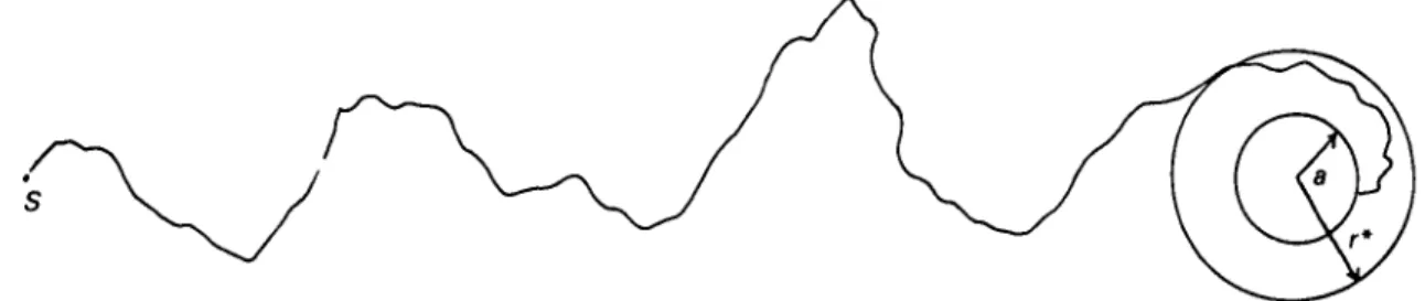
Let us now consider the situation modelized in Figure 1. The device (D) proceeds from a starting point S to a final destination T (target) concretized here by a circle of radius a (the precision circle). D travels toward T by discrete steps of length / and mean velocity v. Hence the mean time duration between two steps A is simply A = lv~l. The motion is stopped when for the first time
the trajectory of D hits the circle T. After each step, the LNP readjusts (if necessary) the orientation of the heading. Indeed, random fluctuations induce a random yaw and then the steps almost never point exactly toward the center of the target; rather, the direction of the steps are randomly distributed according to a probability law. To illustrate these ideas, let us again take the example of an AMR: The size of the gravel on the road on which the robot is rolling will strongly influence the statistics of the errors in the heading and then determine the probability law.
The above qualitative description is now made more precise by the introduction of the following mathematical modelization. Similarly to ref. 3, we specify the dynamics induced by the LNP is assumed to be decomposable into two stages, (Figures 1 and 2 specify the notations). We shall always work in polar coordinates with the origin at the center of T.
a) During the time duration A = lv~\ D moves a distance 6(r, 6) toward the center of the target circle T. The heading 8(r, d) can generally depend on the location of D. For instance, A = Lu~1 can be larger
Fig. 1. Geometry of the problem.
when D is far from T, in this case, we have A(r,) > <5(r2) if r, > r2.
b) Due to the presence of random noise, the deterministic motion described in a) is corrupted by a length ox(r, 0 ) Q , V A in the direction pointing toward the
center of T and by o2{r, 0 ) Q2V A in the perpendicular
direction. Both Q, and Q2 a re taken to be independent Gaussian random variables with zero mean and unit variance. The above choice of the modelization of the noise is motivated, on one hand, by the Central Limit Theorem3 and, on the other hand, by the fact that in the limit A—*dt infinitesimal; we then obtain a diffusion behaviour (the variance of the noise proportional to time). In fact, for a very short time duration A, our noise converges to the Gaussian White Processes (GWP) which often constitute a good idealization of real situations and permit the use of a powerful stochastic analysis.
Hence, the equations of the motion of D take the form (see Figures 1 and 2):
dr = r - r' = r - [(r - A(r, d)f + o\(r, d)Q\A
where:
A(r, 0) = 8(r, 0) + ax{r, 0)Q,\/A.
and
dd = 6-d'= Atg(o2(r, 0)Q2VA[(r - A(r, 0))2
]-05). (lc)
(la) (lb)
By a Taylor expansion of equations (la) and (lc) up to second order, we obtain:
dr = -d(r, 0)A + (2r)~lol(r, 0)Q2A
and
d9 = r~2ox{r, 6)o2(r,
+ r~lo2(r,
where o(A) is such that:
(2a)
(2b)
From now on, we shall consider the regimes for which the length / and the mean velocity v are such that the step duration A shrinks to zero, namely we shall have
£±—>dt an infinitesimal time. In this limit, the noise is the
WNP and equations (2a, b) are Stochastic Differential Equations (SDE) of the Ito type. This process (r, 0) is therefore a diffusion on the plane.3'4 Hence we can write:
6) + (2r)-lo22(r, d)]dt 0)
and
r, 6)dW2j.
(3a)
(3b) where dWk,; k = l,2 are independent WGP (i.e. formal
derivative of the Wiener process) for which we have:4
E(dWkil) = 0; A: = 1, 2, (4a)
T\); k,l = 1,2, (4b)
where E(-) denotes expectations.
Remark that to write equations (4a, b), we made use of the property:4
dWk,tdW,,, = (5)
The set of equations (4a, b) defines a diffusion process whose solutions are Markovian (i.e. once the present state of the system is known the past and the future are stochastically independent).4 Therefore, the dynamics is now completely characterized by the Transition Probabi-lity Density (TPD) P(r, 0, t \ r0, 0O, t0).
The TPD denotes the probability density to find the system at the position (r, 0) at time / by knowing that it was at (r0, 0O) at time t0. For a diffusion process, such as
equations (4a, b), the TPD obeys to a linear partial differential equation naomely the Fokker-Planck-Kolmogorov (FPK) equation 4 which here reads as: lim A-»0
|
n'.e,
1 rQ, 0O) t0) = F(P(r, 0, t \ r0, 0O, t0)). (6a) circle of confusion. circle of precision, 7". Mr, 0)and
f{r, 6) = -6(r, 6) + (2r)-
loi(r, 6).
(6c) The dynamical model is now completely characterised by equations (3a, b) at the level of the realizations of trajectories and by equations (6a, b, c) at the level of probabilities.The questions to be answered for this dynamics can be formulated as follows:
i) What is the probability of the first access time to the target circle Tl
ii) What the distribution of the impact point on the target circle 77
iii) How to qualitatively and quantitatively distinguish between efficient and poorly efficient approaches to the target circle Tl
3. CHARACTERIZATION OF THE
APPROACHES TO THE TARGET CIRCLE From now on we shall restrict our discussion to cases with a cylindrical symmetry, that is to say:
and
With the the above assumptions, it is obvious that equation (3a) is decoupled from equation (3b). Hence, the stochastic process r(t) can be discussed independ-ently of the angle 6(t) a feature which considerably simplifies the analytical discussion. Since equations (3a, b) apply to a diffusion process, this enables us to calculate explicitly the following important quantities:
(a) Stationary probability measure
With the assumptions equations (7a, b, c), the radial part of the diffusion process equations (3a, b) obeys the FPK equation:
- P(r, 11 r
0, t
0) = F- P(r, t \ r
0, t
0), (8a)
at at
8(r, 6) = 8(r),
o
x(r, 6) = a,(r),
O2(r, 6) = O2(r). (7a) (7b) (7c)with the radial FPK operator:
Fo=— l i l ^ n n
dr 2 dr2
The stationary (i.e. time-independent) solution of equation (9) reads:
(8b)
Ps(r) = Na;\r) exp [2 £ oT
2(z)f(z) dz\,
(9)
where N is a normalization constant, (we assume here that N <<*>). From equation (9), we can immediately
-8(r)
- ~ o ? ( r ) |w. = 0. (10b)(b) Mean access time to the target circle 3 5
Starting at a distance R from the center of T, the moments of the first access time to the target E(r"(R)) obey to the equation:
^-
2E(r"(R))+f(R)4
EE(r"(R))
with the boundary conditions:
E(r"(R = a)) = 0.
= 0, (11a)
(lib) In particular, the mean first access-time to the target circle is the solution of equation (lla, b) for n = 1 which reads as:
E(r(R)) = 2 f [oi(co)P
s(co)]-l
\ f P
s(z) dz] do. (12)
Ja L J(O -I
(c) Joint distribution of the first access time and impact angle on the target circle T3
Starting at distance R from the center of T at time t = 0 and angle 6 = 0, the joint distribution of the first access-time (t(R)) and the contact angles (<!>(/?)) of the impacts on the target circle T will be written as
P(T, $ IR, 6 = 0). The generating function L(s, m\R,6)
defined by:
L(s, m\R,6 = 0)
= L(s, m I R) = £[exp (-ST) COS (m R, 6 = 0). (13)
itself obeys a differential equation of the form:
^ 5 Us, m\R)
1a\{R) - 6(R)]
x TT; L(s, m IR) - [s + (2R2)-1o22(R)m2]L(s, m \ R) = 0,
(14) with the the obvious boundary conditions:
L(s, m\R = a) = l, (15a)
lim L(s, m\R) = 0. (15b) and
Two types of approaches to the target T can be characterized by using the most probable radius r* defined by equation (10b). Indeed, when D is at a distance r>r*, it has a net tendency to approach the target circle, while when r<r* this net tendency is reversed, and due to the noise, D feels, in this last case, an effective centrifugal force. In the following, the circle
Fig. 3. Typical trajectory in an inefficient approach. can distinguish the following situations:
a) r*>a (i.e. the circle of confusion is larger than the circle of precision). In this case, D has a pronounced tendency to travel around the target (Figure 3). The
approach is inefficient.
b) r* <a (i.e. the circle of confusion is smaller than the circle of precision). Here, D proceeds mostly in a straightforward way to the target and the tortuous travel around T is comparatively highly improbable. Hence, in
this regime, the approach is efficient (Figure 4).
More refined information is given by the expression equations (11), (12) and (14). While the mean access-time E(r) given by equation (12) is rather easy to evaluate, the solutions of equations (lla) and (14) are usually harder to calculate explicitly. For instance, it is easy to realize that equation (14) is equivalent to a quantum mechanical stationary Schroedinger equation with a general potential. Obviously, powerful ap-proximation techniques are available if a particular situation has to be analysed.
As an illustration, let us confine our discussion to the simplest case and probably the most frequent situation for which we have:
and (16)
(17)
(18) where the radius of the circle of confusion r* according to equation (10b) here reads:
6(r) = d = const, ot(r) = o2(r) = a = const.
In this case, equation (12) simply reads as:
E(r(R)) = (fi-
!)[/? - a + r* log (*)],
r* = a"2(2<5). (19) In equation (18) the contribution 6 *[/? - a] simply corresponds to the ideal (noiseless) access time to reach
T; (remember D starts at distance R from T and travels
at heading velocity 6). Therefore the logarithmic correction present in equation (18) originates from the
noise. The relative magnitude of this term in actual applications, indicates directly how important the fluctuations are and hence, whether they should be really taken into account.
Finally, with the technique reported in ref. 3, the solution of equation (14) with the assumptions equations (16) and (17), can also be given explicitly in terms of hypergeometric functions. Consequently, the distribution of the impacts on the precision circle T can be explicitly given for this case. We refrain to write here the explicit forms of these expressions but mention that the regimes of approaches introduced earlier are explicitely observed at the level of the distribution of impacts on T; (i.e. efficient approach implies a sharply peaked distribution on the ideal (noiseless) linking direction from S to the center of T contrary to the inefficient case, for which the distribution tends to be uniform on T. This is obviously a consequence of the highly probable travel of the device before its contact with the target.
4. CONCLUSIONS
We explore the possibility to take into account the influence of random disturbances on the motion of automated target-seeking devices, such as automated mobile robots. Our modelization of the randomness is made in terms of random white noise which leads us to formulate a dynamics by simple stochastic differential equations. The parameters which enter into the description are the heading mean velocity and the variance of the (assumed) Gaussian noise which has to be measured or estimated.
For this type of dynamics, we propose to distinguish two regimes of approach to the target. To this end, we use the concept of a confusion circle, the radius of which is easy to calculate. It depends in a simple manner on the parameters characterizing the dynamics. When the precision circle (size of the target) is larger than the confusion circle, the approach is efficient. On the other hand, when the precision circle is smaller than the confusion circle a high tortuous travel probability around
advantage of providing an estimation prior to computer simulations which, in any cases, would be unavoidable in any actual particular realizations.
Acknowledgements
We are sincerely grateful to Prof. Dr. C.W. Burckhardt for both his interest and encouragements which stimulate this work.
navigation". J. Royal Stat. Soc. B36, 365-417 (1974). 4. C.W. Gardiner, Handbook of Stochastic Method for
Physics. Chemistry and the Natural Sciences. Springer
(1981).
5. S. Karlin and H.M. Taylor, A Second Course in Stochastic
Processes (Acad. Press New York, 1981), See in particular