Publisher’s version / Version de l'éditeur:
Proceedings of the 16th IAHR International Symposium on Ice, 2, pp. 194-202, 2002-12-02
READ THESE TERMS AND CONDITIONS CAREFULLY BEFORE USING THIS WEBSITE. https://nrc-publications.canada.ca/eng/copyright
Vous avez des questions? Nous pouvons vous aider. Pour communiquer directement avec un auteur, consultez la
première page de la revue dans laquelle son article a été publié afin de trouver ses coordonnées. Si vous n’arrivez pas à les repérer, communiquez avec nous à [email protected].
Questions? Contact the NRC Publications Archive team at
[email protected]. If you wish to email the authors directly, please see the first page of the publication for their contact information.
NRC Publications Archive
Archives des publications du CNRC
This publication could be one of several versions: author’s original, accepted manuscript or the publisher’s version. / La version de cette publication peut être l’une des suivantes : la version prépublication de l’auteur, la version acceptée du manuscrit ou la version de l’éditeur.
Access and use of this website and the material on it are subject to the Terms and Conditions set forth at Temperature Changes in First Year Arctic Sea Ice During the Decay Process.
Johnston, Michelle; Timco, Garry
https://publications-cnrc.canada.ca/fra/droits
L’accès à ce site Web et l’utilisation de son contenu sont assujettis aux conditions présentées dans le site
LISEZ CES CONDITIONS ATTENTIVEMENT AVANT D’UTILISER CE SITE WEB.
NRC Publications Record / Notice d'Archives des publications de CNRC:
https://nrc-publications.canada.ca/eng/view/object/?id=02f88ffc-4da0-4c54-89dc-93d6e23a911b https://publications-cnrc.canada.ca/fra/voir/objet/?id=02f88ffc-4da0-4c54-89dc-93d6e23a911b
Ice in the Environment: Proceedings of the 16th IAHR International Symposium on Ice Dunedin, New Zealand, 2nd–6th December 2002
International Association of Hydraulic Engineering and Research
TEMPERATURE CHANGES IN FIRST YEAR ARCTIC SEA ICE
DURING THE DECAY PROCESS
M. Johnston1 and G.W. Timco1 ABSTRACT
Measurements of the seasonal deterioration of landfast, first year sea ice were made in McDougall Sound, Eastern Canadian Arctic, from early May to July 2002. Ice temperatures were obtained from a temperature chain that was frozen into the ice. The uppermost 0.40 m of ice responded to short-term fluctuations in air temperature. Ice below a depth of 0.50 m showed longer-term response to the steady increase in air temperature. During the decay process, the winter profile of increasing ice temperature with increasing depth reversed; the upper ice surface was warmer than the bottom ice. A systematic increase in ice temperature was observed in ice at all depths. Warming rates decreased linearly from top to bottom, from 0.26°C/day to 0.03°C/day respectively. An analysis showed that the rate of ice decay could be approximated knowing the air temperature/ice surface temperature, ice thickness, and its depth-dependent warming rate.
INTRODUCTION
The Canadian Ice Service is developing a product that provides information on the state-of-decay (ice strength) of level first-year sea ice, in support of the Arctic Ice Regime Shipping System (Gauthier et al., 2002). Typically, ice property measurements have been conducted before mid-May, when the ice is still cold and access to the ice is straightforward. Data on the properties of warming sea ice during its decay process are extremely limited. As a result, a series of studies were undertaken to measure the properties of first year sea ice between late winter and mid-summer. Three seasons of strength and property measurements have been conducted on landfast, first year sea ice near Truro Island (75o14’N, 97o09’W) Nunuvut (Johnston et al. 2001, 2002). This paper examines these detailed ice temperature measurements in an effort to develop a methodology to predict the rate of decay of the ice from the measured air temperature.
AIR TEMPERATURE AND SNOW/ICE THICKNESS DURING 2002 SEASON
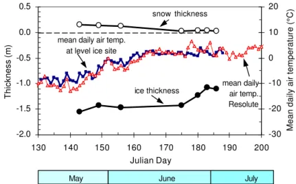
Figure 1 shows the snow depth and ice thickness in relation to air temperature at the ice site near Truro Island. Mean air temperatures from the ice site and those from Resolute agree favorably until 25 June (Julian Day, JD176). The ice thickness during the 2002 season ranged from 1.43 to 1.55 m from mid-May until late-June. In late-June (JD166), once the 0.15 m thick snow had melted, the ice began to decrease in thickness. This agrees with
Timco and Johnston (2002) who state that ice properties change dramatically after snow melt and after air temperatures remain above 0°C for about one week.
The ice was just over one metre thick when the final ice property measurements were made on 5 July (JD186). The ice thickness decreased
0.33 m in 11 days, or about 30 mm/day, which agrees well with previous ice ablation rates of 34 mm/day and 22 mm/day (Johnston et al., 2002).
DEVICE USED TO MEASURE ICE TEMPERATURES
The decrease in ice thickness was initiated by temperature changes throughout the full-thickness of ice. Realizing the importance of accurate measurements of in situ ice temperatures, considerable effort was spent developing an array of temperature sensors prior to the 2002 field season.
Fabrication of Temperature Chain
The temperature chain consisted of a string of Type T shielded thermocouples, mounted inside a 50 mm white, PVC pipe. During assembly, care was taken to minimize the influence of embedding foreign materials (with different thermal properties) in the ice. The temperature chain was assembled using an “open concept” in that as much material as possible was removed from the PVC pipe during its assembly. A slot was made down one side of the pipe and a series of holes was drilled in the opposite side, ensuring that the sensors were surrounded by ice.
The thermocouples were spaced at 0.10 m intervals to an ice depth of 0.9 m. Intervals of 0.20 m were used between ice depths 0.90 m and 1.7 m. The array included three cross checks on the measured temperatures. First, the uppermost sensor was installed at a distance of 0.10 m above the ice surface. Measurements from that thermocouple were compared with temperature measurements made inside the insulated data logger box. By design, at least one thermocouple remained in seawater at all times to provide a record of the sea water temperature (itself a reference point). The third cross check involved using a Campbell Scientific thermilinear temperature probe (thermistor, 44212B-L) at the same depth as one of the thermocouples (ice depth 1.1 m). Measurements from the thermistor and thermocouple were made independently. Comparison of the two temperature sensors made in the laboratory before shipment showed that the two sensors agreed to within 0.1°C. In the field, the sensors agreed to within 0.3°C throughout the season.
Figure 1: Ice conditions during the 2002 field program
-2.0 -1.5 -1.0 -0.5 0.0 0.5 130 140 150 160 170 180 190 200 Julian Day Thickness (m) -30 -20 -10 0 10 20
Mean daily air temperature (°C)
May June July
snow thickness
ice thickness mean daily air temp. Resolute mean daily air temp.
Installation of Temperature Chain
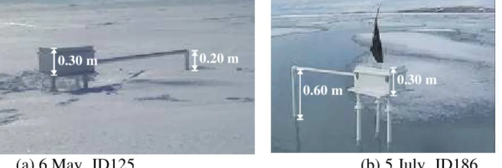
A site was selected that was in an area of level first year ice that was close to, but unaffected by the ice property measurement site. Once a site had been selected for the temperature chain, a 50 mm hole was drilled through the full thickness of the ice. Ice thickness at the time of installation was 1.44 m. The temperature chain was inserted into the hole and positioned at the appropriate depth, with the second thermocouple in the chain at the snow-ice interface (the snow-snow-ice interface was 0.30 m from the top of the PVC pipe). By the time the site was re-visited, the chain had frozen solidly into the ice. At that point, lead wires from the thermocouples/thermistor were wired into a Campbell Scientific CR10 data logger. The logger was placed in an insulated box and mounted on a raised platform, about 1.5 m from the temperature chain itself (Figure 2). Elevating the enclosure ensured that it did not act as a snow catch and it also minimized the effect (upon the temperature sensors) of melt around the platform legs, which were embedded in the ice. On 11 May (JD131) the data logger was activated and sampling began at all depths. The sampling interval was once every 30 minutes.
Figure 2a shows the temperature chain after it was installed on 6 May (JD125). Initially, there was about 100 mm of snow covering the ice. Temperature measurements were first logged on 11 May (JD131) and measurements were terminated on 5 July (JD186). Figure 2b shows the temperature chain when it was retrieved on 5 July (JD186). At that point, the ice around the temperature chain had melted to an “ice” depth of -0.30 m. The melt pond was the reason for the divergence on JD175 between temperature from the ice site and the weather station (Figure 1). Clearly, by the end of the field season, the first six sensors were measuring the temperature of the surrounding melt pond. The chain was still frozen into the ice when it was removed on JD186.
0.60 m 0.30 m
0.30 m 0.20 m
(a) 6 May, JD125 (b) 5 July, JD186
Figure 2: Temperature chain and data logger at (a) beginning and (b) end of season
TYPICAL FULL-THICKNESS ICE TEMPERATURE PROFILES
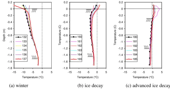
Three five-day periods were selected to provide “snapshots” of the ice temperature profiles between May and July 2002. Those three stages were identified as winter, melt, and advanced melt.
Case I: Winter
Figure 3a shows that, in mid-May (JD132 to 137), the top of the ice was much colder than the bottom of the ice. On 12 May (JD132) the upper ice surface had a temperature of –10°C whereas the temperatuare at the ice-water interface was about –1.8°C (sensors at 1.5 and 1.7
m were submerged in seawater). Ice with a temperature that increases linearly with increasing depth is typical of cold, winter sea ice.
-1.8 -1.6 -1.4 -1.2 -1 -0.8 -0.6 -0.4 -0.2 0 0.2 -15 -10 -5 0 5 Temperature (°C) Depth (m) 132 133 134 135 136 137 -1.8 -1.6 -1.4 -1.2 -1 -0.8 -0.6 -0.4 -0.2 0 0.2 -15 -10 -5 0 5 Temperature (°C) Temperature (C) 160 161 162 163 164 165 -1.8 -1.6 -1.4 -1.2 -1 -0.8 -0.6 -0.4 -0.2 0 0.2 -15 -10 -5 0 5 Temperature (°C) Temperature (C) 180 181 182 183 184 185
(a) winter (b) ice decay (c) advanced ice decay
Figure 3: Full-thickness profiles of temperature (cross hatches indicate ice top/bottom) Case II: Ice Decay
By the middle of June (JD160 to 165) the temperature profile of the ice had changed considerably from its winter state. Figure 3b shows that the ice was warmer at all depths. The change in temperature, however, did not vary uniformly with depth. The uppermost 0.20 m of ice had warmed to the extent that it was warmer than the interior ice, the reverse of ice in its winter state. Ice between depths 0.20 to 0.70 m was virtually isothermal at – 2.8°C. Ice below a depth of 0.70 m was characteristic of winter ice in that its temperature increased with increasing depth.
Case III: Advanced Ice Decay
Figure 3c shows the temperature profile for ice during the first week of July (JD180 to 185). Sensors to a depth of –0.30 m had temperatures above 0°C. The reason for high temperatures at those depths was that those sensors were recording the temperature of a melt pond, shown in Figure 2b. Meaurements below that depth showed that ice at all depths had temperatures above –1.0°C during an advanced stage of decay. The temperature of ice in an advanced stage decreased with increasing depth throughout the full depth of ice. The temperature gradient throughout the full-thickness ice was opposite of that during the winter period.
PROPAGATION OF SHORT-TERM CHANGES IN AIR TEMPERATURE
The surface layer of ice is now examined in detail to determine the depth to which fluctuations in air temperature, or thermal waves, penetrate the ice. That depth will be designated as the “active layer” of ice.
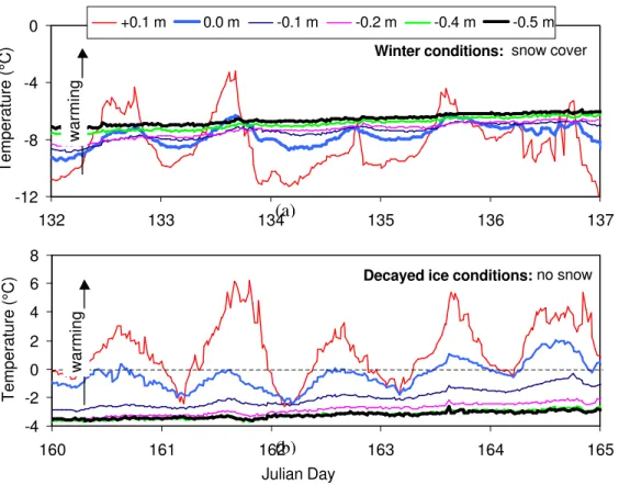
Temperatures in the uppermost 0.50 m of ice are shown in Figure 4 for ice in its winter state (Figure 4a, JD132 to 137) and ice in a decayed state (Figure 4b, JD160 to 165). Temperature readings were taken every 30 minutes. The depth +0.10 m refers to the thermocouple that was 100 mm above the snow-ice interface. Since the snow depth was 50
to 80 mm when the temperature chain was installed on JD132, the uppermost sensor recorded air temperatures from the start.
The air temperature (+0.10 m) peaked at about mid-day. Ice in its winter state (Figure 4a) had a thick snow cover that limited the effects of fluctuating air temperature to the uppermost 0.20 m of ice. During the winter period, short-term changes in air temperature had negligible effect on ice below a depth of 0.20 m. For instance, on JD133, a diurnal change in air temperature of 7°C caused a diurnal change of 2.3°C at the snow-ice surface (0.0 m). There was corresponding change of 1°C in the ice at depths of –0.10 and –0.20 m. During its winter state, temperature changes beneath the top ice were both attenuated and delayed (by several hours) compared to changes in the air temperature. Ice below a depth of –0.30 m did not show an immediate response to daily changes in air temperature, however it did have a long-term response. Over the five-day period, ice at depths –0.30 m, -0.50 m and –0.90 m (not shown) increased by 1.3 °C, 1.2°C and 0.4°C respectively.
-12 -8 -4 0 132 133 134 135 136 137 Julian Day Temperature (°C) +0.1 m 0.0 m -0.1 m -0.2 m -0.4 m -0.5 m warming
Winter conditions: snow cover
-4 -2 0 2 4 6 8 160 161 162 163 164 165 Julian Day Temperature (°C)
Decayed ice conditions: no snow
warming
Figure 4: Propagation of short-term changes in air temperature
During the decayed state, only a few millimeters of snow covered the ice. For all intents and purposes, the snow cover did not exist, which allowed changes in air temperature to penetrate further into the ice (Figure 4b). On JD160 there was an 8°C diurnal change in air temperature. Ice in the surface layer showed effects from that temperature change; there was also a diurnal response of 0.2°C at a depth of –1.10 m (not shown). Ice in a decayed state allowed thermal waves to propagate throughout the ice cover. The thermal waves
(a)
propagated throughout the ice with no significant delay in the diurnal temperature peaks at the different depths.
PROGRESSIVE WARMING OF THE ICE DURING DECAY PROCESS
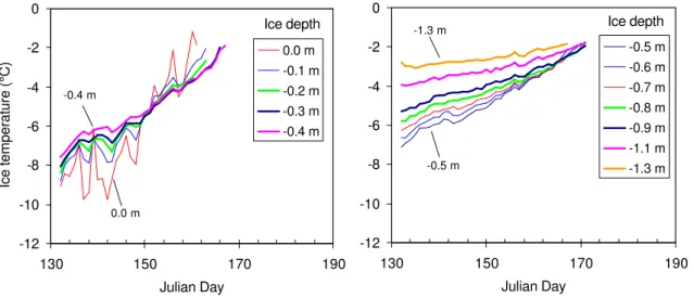
The previous figures showed that there was a steady warming of ice at all depths. The overall increase in temperature, and its corresponding rate of increase depended, however upon the particular ice depth. Figure 5 illustrates the progressive warming that occurred at different ice depths during the decay process. Only those temperatures recorded each day at 06:00 hours were included in the figure.
-12 -10 -8 -6 -4 -2 0 130 150 170 190 Julian Day -0.5 m -0.6 m -0.7 m -0.8 m -0.9 m -1.1 m -1.3 m Ice depth -1.3 m -0.5 m -12 -10 -8 -6 -4 -2 0 130 150 170 190 Julian Day Ice temperature (°C) 0.0 m -0.1 m -0.2 m -0.3 m -0.4 m Ice depth -0.4 m 0.0 m
Figure 5: Ice temperature for all depths, until a temperature of -1.8°C is reached Figure 5 shows that temperatures at all ice depths converged to about –1.8°C between 16 and 20 June (JD167 to JD171). Once the full-thickness ice cover had a uniform temperature of –1.8°C, the ice can be considered to be in an advanced state of decay. As a result, Figure 5 only includes temperatures before the date on which ice at different depths warmed to –1.8°C. Measurements above this temperature are difficult to interpret since they could be influenced by localized melting around the sensor tip, and thus, not necessarily be representative of the local ice temperature.
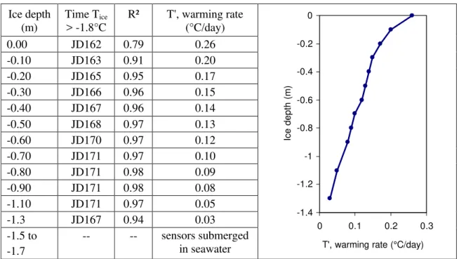
As expected, the largest amount of warming (and most erratic) occurred at the snow-ice interface. Before the ice surface reached –1.8°C and entered an advanced stage of decay, its temperature had to warm by 8°C. In comparison, ice at a depth of –1.3 m needed to increase by only about 1°C before it could be characterized as ice in an advanced state of decay. Taking the slope of the curves plotted in Figure 5 would provide an indication of the rate of temperature change, T' (°C/day) or warming rate, that was characteristic for ice at different depths. This was done by fitting a linear regression to each temperature-time curve and then tabulating the results. The slopes of the linear regressions are shown in Table 1. Omitted from the table are the y-intercepts corresponding to the linear regressions, which ranged from –1.4 to 0.01. The R² values shown in Table 1 were used to indicate the goodness of fit between the actual data and the regression. The R² values range from 0.79 (in the top ice) to 0.98 at depths 0.80 and 0.90 m, demonstrating the feasibility of a linear regression in approximating the actual temperature measurements.
There was a uniform decrease in warming rate, T', with increasing ice depth as shown graphically in Table 1. The plot of T' illustrates the uniformity of the warming rate with depth and also gives an idea as to how the warming front progresses from the upper and lower ice surfaces. The dates on which the ice temperatures warmed to –1.8°C provide evidence of the warming trend. Note that the upper and lower ice surfaces reached a temperature of –1.8°C before the ice interior. Interestingly, ice depths between –0.70 m to – 1.10 m increased to –1.8°C on the same day (JD171).
Table 1: Warming Rate, T' Ice depth (m) Time Tice > -1.8°C R² T', warming rate (°C/day) 0.00 JD162 0.79 0.26 -0.10 JD163 0.91 0.20 -0.20 JD165 0.95 0.17 -0.30 JD166 0.96 0.15 -0.40 JD167 0.96 0.14 -0.50 JD168 0.97 0.13 -0.60 JD170 0.97 0.12 -0.70 JD171 0.97 0.10 -0.80 JD171 0.98 0.09 -0.90 JD171 0.98 0.08 -1.10 JD171 0.97 0.05 -1.3 JD167 0.94 0.03 -1.5 to -1.7 -- -- sensors submerged in seawater -1.4 -1.2 -1 -0.8 -0.6 -0.4 -0.2 0 0 0.1 0.2 0.3 T', warming rate (°C/day)
Ice depth (m)
PROGRESSION OF ICE DECAY: ACTUAL VERSUS PREDICTED
Ice at all depths showed a warming trend throughout the season. Is it possible to establish a temperature profile that can be used to relate the ice surface temperature to temperature in the interior of the ice? If so, information about the temperature of the ice could be used as a proxy for determining the ice strength during the decay process.
If one wanted to predict the progression of ice decay, information about the ice conditions would need to be available. Since ice temperatures are seldom known, one would need to rely upon air temperatures records. This section presents the results of an analysis in which the date of ice decay was predicted using an initial temperature measurement from a) the ice surface, and b) the Resolute weather station.
Figure 6a shows the actual temperature gradient, ∇Tiact, that initially existed in the ice. Data
for ∇Tiact curve were obtained by averaging the 30-minute temperatures recording over the
course of JD132. Two techniques were used to approximate the actual temperature profile. In the first case, the linear temperature gradient, designated as ∇Tisurf, shows an ice surface
because both used measurements from an ice depth of 0.0 m on JD132. The second approximation, ∇Tiair, shows a starting ice surface temperature of –10°C as obtained from
the 5-day average of the mean daily air temperature at Resolute. In all cases, the temperature of the ice decreases with increasing depth to a value of –1.8°C at a depth of 1.44 m (the ice thickness on JD132). Note that ∇Tiair provides a better approximation of the
actual temperatures than ∇Tisurf., except in the uppermost 0.40 m. Deviation of the actual
ice temperature from the linear profile (typical of cold, winter sea ice) shows that the ice had already begun to warm on JD132. The right-hand side of Figure 6a shows the final temperature profile in the ice, obtained from actual measurements (∇Tfact) and the predicted
temperature profile (∇Tpred). In both cases, the full thickness of ice has a uniform
temperature profile of about –1.8°C.
-1.5 -1.0 -0.5 0.0 -10 -8 -6 -4 -2 0 Temperature (°C) Ice depth (m) Tiair Tfact Tisurf Tiact Tfpred -1.5 -1.0 -0.5 0.0 20 30 40 50 Time, ∆t (days) Ice depth (m) t surf t air t act (a) (b)
Figure 6: (a) Temperature profiles and (b) actual and predicted times (∆t) to –1.8°C (hatches show ice surface)
The change in temperature between the initial (∇Ti) and final state of the ice (∇Tf) was
calculated for each ice depth. The amount of warming (°C) required for each ice depth to reach its final state was multiplied by the rate of warming, T' (°C/day), for each depth (see Table 1). That simple calculation was a first approach towards predicting the time required for different layers of ice to reach an advanced state of ice decay (ice temperature of – 1.8°C). The results of those calculations are shown in Figure 6b.
The actual time required for different ice depths to reach –1.8°C was denoted as ∆tact, which
is the number of days between JD132 and the dates listed in Table 1. Results of the calculations for the predicted time using the measured ice surface temperature (∆tsurf) and
the prediction using the air temperature (∆tair) are shown in Figure 6b. Results show that the
number of warming days required in the surface layer of ice (depth 0.40 m) was best
approximated using the measured ice surface temperature (∇Tisurf in Figure 6a). In
comparison, ice depths below 0.60 m were better characterized by the 5-day average of air temperature (∇Tiair in Figure 6a). It is emphasized that Figure 6 is based on an investigation
FINAL COMMENTS
This analysis has shown that it is possible to estimate the internal temperature profile in an ice sheet, and its change with time, from the air temperature history. However, the internal decay is not a simple process, so a two-part methodology is required. Further studies are being conducted to supplement these data and to determine their relevance to other geographic regions. If this methodology can be further substantiated, it will be a very useful approach for predicting the state of ice decay.
ACKNOWLEDGEMENTS
This research was sponsored by Transport Canada and the Canadian Ice Service. The authors would like to thank V. Santos-Pedro and R. DeAbreu for their interest in this work. The field assistance of Canadian Ice Service, University of Manitoba, University of Calgary, and the Polar Continental Shelf Project is much appreciated.
REFERENCES
Gauthier, M-F., DeAbreu, R., Timco, G.W. and Johnston. M.E. Ice Strength Information in the Canadian Arctic: From Science to Operations. Proceedings IAHR Ice Symposium (this volume), ( 2002), Dunedin, New Zealand.
Johnston, M., Frederking, R. and Timco, G. Properties of Decaying First Year Sea Ice: Two Seasons of Field Measurements. Proceedings 17th International Symposium on Okhotsk Sea and Sea Ice, pp 303-311, (2002), Hokkaido, Japan.
Timco G. and Johnston, M. Sea Ice Strength during the Melt Season. Proceedings 16th
International Symposium on Ice (this volume), (2002), Dunedin, New Zealand. Johnston, M., Frederking, R. and Timco, G. Decay-Induced Changes in the Physical and
Mechanical Properties of First Year Ice. Proceedings 16th International Conference on Port and Ocean Engineering under Arctic Conditions, pp 1395-1404, (2001), Ottawa, Canada.