HAL Id: hal-00153958
https://hal.archives-ouvertes.fr/hal-00153958
Submitted on 25 Jan 2021
HAL is a multi-disciplinary open access
archive for the deposit and dissemination of
sci-entific research documents, whether they are
pub-lished or not. The documents may come from
teaching and research institutions in France or
abroad, or from public or private research centers.
L’archive ouverte pluridisciplinaire HAL, est
destinée au dépôt et à la diffusion de documents
scientifiques de niveau recherche, publiés ou non,
émanant des établissements d’enseignement et de
recherche français ou étrangers, des laboratoires
publics ou privés.
The coupled physical-biogeochemical system in the
equatorial Pacific in sept-nov 1994
Anne Stoens, Christophe E. Menkès, Marie-Hélène Radenac, Yves
Dandonneau, Nicolas Grima, Gérard Eldin, Laurent Mémery, C. Navarette,
Jean-Michel André, T. Moutin, et al.
To cite this version:
Anne Stoens, Christophe E. Menkès, Marie-Hélène Radenac, Yves Dandonneau, Nicolas Grima, et al..
The coupled physical-biogeochemical system in the equatorial Pacific in sept-nov 1994. Journal of
Geo-physical Research, American GeoGeo-physical Union, 1999, 104 (C2), pp.3323-3339. �10.1029/98JC02713�.
�hal-00153958�
JOURNAL OF GEOPHYSICAL RESEARCH, VOL. 104, NO. C2, PAGES 3323-3339, FEBRUARY 15, 1999
The coupled physical-new production system in the equatorial
Pacific during the 1992-1995 El Nifio
Anne
Stoens,
• Christophe
Menkbs,
• Marie-H61bne
Radenac,
• Yves Dandonneau,
•
Nicolas
Grima,
• G6rard
Eldin,
2'
3 Laurent
M6mery,
• Claudie
Navarette,
2
Jean-Michel
Andr6,
2 Thierry
Moutin,
4 and Patrick
Raimbault
4
Abstract. We investigate
the coupling
between
the physics
and new production
variability
during
the period April 1992 to June 1995 in the equatorial
Pacific via two cruises
and
simulations.
The simulations
are provided
by a high-resolution
Ocean General Circulation
Model
forced
with satellite-derived
weekly
winds
and
coupled
to a nitrate
transport
model
in
which biology acts as a nitrate sink. The cruises
took place in September-October
1994 and
sampled
the western
Pacific
warm pool and the upwelling
region
further
east.
The coupled
model
reproduces
these
contrasted
regimes.
In the oligotrophic
warm pool the upper layer is
fresh, and nitrate-depleted,
and the new production
is low. In contrast,
the upwelling waters
are colder,
and saltier
with higher nitrate concentrations,
and the new production
is higher.
Along the equator
the eastern
edge of the warm pool marked
by a sharp
salinity front, also
coincides
with a "new production
front". Consistent
with the persistent
eastward
surface
currents
during the second
half of 1994, these
fronts undergo
huge eastward
displacement
at
the time of the cruises.
The warm/fresh
pool and oligotrophic
region has an average
new
production
of 0.9 mmol
NO3 m -2 d -l, which
is almost
balanced
by horizontal
advection
from
the central
Pacific and by vertical advection
of richer water from the nitrate reservoir
below.
In contrast,
the upwelling
mesotrophic
region shows
average
new production
of 2.1
mmol
NO3 m -2 d -l and the strong
vertical
nitrate
input
by the equatorial
upwelling
is balanced
by the losses,
through
westward
advection
and meridional
divergence
of nitrate rich waters,
and by the biological sink.
1. Introduction
The major focus of the Joint Global Ocean Flux Study (JGOFS) international program is devoted to the oceanic carbon cycle and its long-term consequences on the variations of the atmospheric CO• content. Among JGOFS process studies, those concerning the equatorial Pacific were undertaken for several reasons.
First of all, the equatorial cold tongue of upwelled waters has large spatial extension [Wyrtld, 1981]. These waters upwelled from depth are rich in nutrients and in inorganic carbon. High nutrient content enhances photosynthesis, new production of organic carbon, and sedimentation of particles. In addition, the high carbon content of the upwelled waters maintains a high partial pressure of CO• at the sea surface. In relation to this, in this re,on the CO• flux at the air-sea interface goes to the atmosphere, and the Pacific equatorial upwelling is the largest marine source of CO• to the atmosphere [Tans et al., 1990]. This makes the equatorial Pacific a key region for the carbon cycle.
• Laboratoire d'Oc6anographie Dynamique et de Climatologie, (CNRS/ORSTOM/Univ. Paris 6), Paris, France.
2 Institut Francais de Recherche Scientifique pour le D6veloppement en Coop6ration, Noum6a, New Caledonia, France.
3 Now at Laboratoire d'Etudes en G60physique et Oc6anographie Spatiales, Toulouse, France.
n Centre d'Oc6anologie de Marseille, Marseille, France.
Copyright 1999 by the American Geophysical Union.
Paper number 98JC02713. 0148-0227/99/98JC-02713509.00
A second characteristic of the equatorial Pacific is its relatively modest chlorophyll content and low primary
productivity compared to the abundance of nitrate in the
surface layers. The equatorial Pacific upwelled waters have thus been described as high nutrients-low chlorophyll waters (HNLC) [Thomas, 1979] and the roles of iron [Martin, 1990; Barber, 1992] or of grazing [Walsh, 1976] have been
proposed to explain this paradox. However, neither the high
carbon fluxes to the atmosphere and to depth, which are common to all tropical upwelling areas, nor the HNLC character, which is also observed in the Antarctic, are exclusive of the equatorial Pacific.
In contrast, a third property is unique to this region' it
arises from the interannual El Nifio-Southem Oscillation
(ENSO) that affects the world climate. During the warm
phases of this oscillation (El Nifio) the equatorial upwelling
collapses dramatically reducing the biological sink of carbon
associated with new production [Barber and Chavez, 1983;
Dandonneau, 1986] and the CO2 outgasing [Wong et al.,
1984, 1993; Feely et al., 1995; Dandonneau, 1995]. The
study and prediction of ENSO constituted the major goals of
the 1985-1994 international Tropical Ocean Global Atmosphere program (TOGA). In the course of TOGA our
general knowledge of large-scale circulation has been greatly
improved. It is now well known that the variability of the
equatorial Pacific results from basin-wide coupling processes between the ocean and the atmosphere. The circulation of surface water masses, which controls the equatorial
upwelling, is deeply affected by these processes. This
emphasizes the point that the value of biogeochemical
variables at a given position, which results largely from the
3324 STOENS ET AL.' COUPLED PHYSICAL-NEW PRODUCTION SYSTEM
advection of upwelled water, is controlled by these processes and thus cannot be properly understood in a one-dimensional (l-D) view. In particular, horizontal advection is of primary
importance for determining the biogeochemical conditions in
the equatorial Pacific. This complicates the study of the biological fluxes to such a point that certainly, the JGOFS study of the equatorial Pacific would not have been possible without the lessons from TOGA.
During this program, in situ observational networks such
as Tropical Atmosphere Ocean (TAO) have been deployed all over the equatorial Pacific, which deliver, in particular, real- time knowledge of the subsurface thermal structure variations
of the ocean (10øS-10øN) and knowledge of the current along
the equator [Hayes et al., 1991, McPhaden, 1993] so that the
equatorial Pacific Ocean is now the' best observed ocean.
Therefore the international JGOFS study of the equatorial Pacific has benefited from the attainments of TAO. For example, Kessler and McPhaden [1995] used these networks
to describe of the dynamical aspects of the equatorial Pacific
during the period of the U.S.-JGOFS EqPac cruises which sampled the central Pacific Ocean, at 140øW, during a warm
anomaly, and during near-normal conditions in spring and fall
of 1992 respectively.
The western equatorial Pacific has been studied during an Australian-JGOFS cruise in October 1990 [Mackey et al., 1995] during non E1-Nifio conditions. The FLUPAC and OLIPAC JGOFS-France cruises in the western to central equatorial Pacific were made in September-November 1994 when conditions were more characteristic of warm conditions. The latter cruises sampled the ocean in dynamically and biogeochemically contrasted areas. In short, the western equatorial Pacific is characterized by a warm pool region
where surface waters are warmer and fresher than upwelled
waters farther east. This warm pool experiences huge zonal excursions on interannual timescales which are of
fundamental importance for the world climate [Picaut et al.,
1996]. The signature of these two contrasted physical regimes is also reflected in biogeochemistry as seen in Figure 1 where
abundance of 0-500 m integrated mesozooplankton
(>200 !xm) [Le Borgne and Rodier, 1997] as well as other parameters along the equator during FLUPAC increase sharply from the warm pool region to the upwelling region.
This suggests a strong coupling between the physics and
biogeochemistry at the time of the FLUPAC and OLIPAC
cruises.
The main objective of this work is thus to gain knowledge
on the coupled dynamical-biogeochemical processes that are
at work in the settling, in the maintenance, and in the large-
scale displacement of the nutrient poor warm pool and the
adjacent waters in relation to ENSO conditions. Thus we aim
at understanding the main coupled factors that control new
production in the equatorially contrasted waters.
Such knowledge can be gained through observations: for instance, the FLUPAC and OLIPAC cruises were focused on
the estimation of new and exported primary production, in
relation to the dynamics of the ocean. However, as useful as it may be, such informaden provided by the FLUPAC and OLIPAC data is only relevant to the place and time where these cruises took place. In order to understand the observations in the large-scale context, it is necessary to enlarge the scope of the punctual cruises to the basin and to
the seasonal to interannual scales. While synoptic view of the
ocean sea level variations is successfully given by altimeters
such as TOPEX/POSEIDON [Busalacchi et al., 1994; Picaut et al., 1995] and dynamic height is monitored by the TAO network, previous attempts to develop such a comprehensive data set for biogeochemical data are limited to satellite- detected sea color by the Coastal Zone Color Scanner [Yoder et al., 1993] and monitoring using measurements by ships of
opportunity [Dandonneau, 1992]. Therefore the basin-scale
link between the physics and the biology can only be inferred
from coupled models.
In the equatorial ocean where advection processes, especially by zonal currents, are known to be important [Picaut and Delcroix, 1995], 1-D coupled models can generally not account for observed variations, and one needs
to use a 3-D coupled model to desci'ibe the complexity of
observed variability. Coupled biological-physical models in the equatorial Pacific have already been used to study the seasonal variations of the basin and long-term evolution
[Toggweiler and Carson, 1995; Chai et al., 1996].
Toggweiler and Carson, and Chai et al. used climatological
forcing in their simulations which is not appropriate for a case
study focused on the situation encountered at the time of
FLUPAC and OLIPAC or for understanding the coupled
conditions during ENSO period. Similarly, it is not well suited for the study of transient processes such as equatorial
and instability waves which propagate in the equatorial region
and may deeply impact the biology [Murray et al., 1994].
35.50 35.00. 34-.50 34.00 '--' 0.30 • 0.20 C3 O. lO 0.00 •_• 425 • 400 • 375 0 350 .•. 325 ? • 1500 E c 1000 o _o 500 o o N 0 170øE 175øE
FLUPAC - equatorial leg
180 ø 175øW 170øW 165øW 160øW 155øW 150øW
Figure 1. Surface biogeochemical measurements along the
equatorial FLUPAC leg: (a) sea surface salinity, (b) chlorophyll, (c) pCO2 in the ocean, and (d) ash free dry weight of mesozooplankton in the upper 500 m adapted from Le Borgne and Rodier, [ 1997].
STOENS ET AL.: COUPLED PHYSICAL-NEW PRODUCTION SYSTEM 3325
In order to explicitly resolve all these features we use here the high-resolution Ocean General Circulation Model
(OGCM) OPA of the Laboratoire d'Ocranographie
Dynamique et de Climatologie (LODYC) [Blanke and Delecluse, 1993] forced by high-resolution, high-quality remotely sensed European Remote Sensing (ERS)-l scatterometer stresses [Grima et al., 1998] and coupled to a nitrate transport model. By this we aim at simulating the physical-new production interactions during the 1992-1994 weak E1 Nifio period in which FLUPAC and OLIPAC took place.
The paper is thus organized as follows: in section 2, data and model descriptions are given. In section 3 a quick overview of the large-scale variations of the physical conditions from 1992 to 1995 is given from data and model fields. The coupled dynamical-biogeochemical modeled situations during the FLUPAC and OLIPAC cruises are then
compared to data. In section 4 the variations of coupled
dynamical-new production features over the equatorial Pacific
from 1992 to 1995 are studied using the model. It is shown
that new production at the equator experiences a sharp
transition when going from the warm/fresh pool region to the upwelling region and that this transition has large east-west displacements over the basin in association with the ENSO- related east-west displacements of the salinity front at the eastem edge of the warm pool. Finally, discussion about the modeled new production is given, and in section 5 the conclusion is presented.
2. Data and Model
2.1. Materials and Methods Used During FLUPAC and OLIPAC Cruises
The FLUPAC cruise sampled the equatorial Pacific in these two different regimes with a meridional transect along
165øE (20øS-6øN; September 1994), across the oligotrophic waters of the warm pool, and an equatorial section across the eastern edge of the warm pool into the upwelling region (167øE-150øW; October 1994). The OLIPAC meridional transect took place along 150øW (13øS - 1 øN; November
1994).
Temperature and salinity were obtained using a Sea-Bird SBE 911+ Conductivity-Temperature-Depth profiler (CTD). The sensors were calibrated before the beginning of FLUPAC, and salinity data were validated after measurements of discrete samples with a Portasal salinometer. The vertical profiles of temperature and salinity were processed for spike removal and binned every meter using the software provided by Sea-Bird.
Currents were continuously recorded by two acoustic Doppler current profilers (ADCPs) from R. D. Instruments. The two ADCPs used 75 and 300 kHz frequencies, with vertical resolutions of 16 and 4 m and first bins at 28 and
12 m, respectively. The results from the two instruments were in good agreement, so that the two files of data could be merged into a single set of vertical profiles from 12 to 700 m depth.
Nitrate was measured with a Technicon autoanalyzer using the colorimetric method described by Strickland and Parsons [1972]. For low nitrate concentrations this method was improved to detect nitrate at concentrations as low as
0.003 gmole kg '• at FLUPAC [Oudot and Morttel, 1988] and
0.001 gmole kg '• at OLIPAC [Raimbault et al., 1990].
The chlorophyll concentration was measured according to
several techniques (including high-performance liquid
chromatography and spectrofluorometry). The data presented
here, in order to provide an indication of the biological
activity, were obtained using the fluorescence/acidification
technique described by Yentsch and Menzel [1963], where the pigments are extracted by methanol instead of acetone [Herbland et al., 1985]. Filtration was made on Whatman GF/F filters, filtration pressure being kept below 0.15 atm. 2.2. Data From Observations Networks
Among diverse observing systems enhanced or developed during TOGA the TAO array of deep ocean moorings
provides a permanent and synoptic view of the upper ocean
thermal structure with high temporal resolution. Dynamic heights deduced from the TAO data were kindly provided by M. McPhaden and D. McClurg at Pacific Marine Environmental Laboratory (PMEL), National Oceanic and Atmospheric Administration (NOAA). These dynamic heights at mooring positions are interpolated onto a regular 5 ø longitude x 1 o latitude x 1 day grid using objective analysis used in Menkes et al. [ 1995]. Together with these in situ data, the Reynolds and Smith [1994] sea surface temperatures (SSTs) are used.
2.3. The Dynamical Model
The dynamical model we are using is the three tropical oceans version of the OPA-LODYC OGCM [Maes et al.,
1997]. One specificity of this model is the parameterization of vertical diffusion using the 1.5 turbulent kinetic energy (TKE) closure [Blanke and Delecluse, 1993]. This high-resolution (45' longitude x 20' latitude at the equator; 16 vertical levels in the upper 150 m) model is forced with observed weekly stresses deduced from ERS-1 scatterometer [Grima et al., 1998]. There is a good agreement between wind vectors from the ERS-1 scatterometer and winds measured on the TAO buoys [Bentamy et al., 1996; Grima et al., 1998].
To drive the OGCM "OPA7," satellite-derived wind stresses are completed with water and heat fluxes. These fluxes are computed using bulk aerodynamic formulae with stress from ERS-1, Reynolds and Smith's [1994] SSTs, and all other parameters derived from the atmospheric model Arp6ge- Climat [Dequd e! al., 1994] outputs. The OGCM has been forced from mid-1992 to 1995. Overall comparisons between the outputs of the ERS-1 forced OGCM, TAO in-situ data, and satellite observations have been performed for different ocean variables over the equatorial Pacific Ocean [Grima e! al., 1998]. Five-day outputs were analyzed spanning the 1992-1995 period, and during the specific period of FLUPAC and OLIPAC, linear interpolation of five-day outputs to daily values was performed for comparison with data.
2.4. The Coupled Biogeochemical Model
This OGCM is coupled to an off-line tracer nitrate model using the dynamical outputs to solve the advection-diffusion equations [Levy, 1996] on the OGCM grid:
tPNO 3 c9t
...
(u.V)NO3
+ KhANO3
+ 4(-Xz4NO3)
+(
•?NO3
•?t)
biology
3326 STOENS ET AL.: COUPLED PHYSICAL-NEW PRODUCTION SYSTEM
The left-hand term represents the eulerian variation of the tracer (nitrate) and is calculated as the sum of the advection terms (first term in the right-hand side), the horizontal
diffusion terms (this one is quasi-negligible here), vertical
diffusion terms, and the biological sink. Currents and diffusion coefficients are taken from the dynamical
simulation. The last term represents the biological nitrate sink
(biological model). As in the host physical model, the
governing equations are solved on a C grid. An absolute requirement is that the biological tracer concentrations remain
positive. Therefore a positive definite advection transport
scheme [Smolarkiewicz and Clark, 1986] is used to compute
advection.
Previous attempts to represent the biogeochemistry in the
equatorial Pacific [Toggweiler and Carson, 1995; Chai et al., 1996] were based on a biological model where the phytoplankton, the zooplankton, ammonium, and detritus
were explicit compartments where the nitrogen fixed by
photoautotrophs could accumulate. However, the field data
and experimental knowledge to initialize these compartments
and adjust the fluxes between each other are uncertain. Since we focus here on new production [Dugdale and Goering, 1967] we choose to reduce the ecosystem to a single nitrate compartment. Thus, in this simple system the new nitrate that is taken by the photoautotrophs cannot be stored in any compartment in the photic layer and must then be immediately remineralized at depth. This procedure presents the inconvenience of a too strict coupling between new production and remineralization that does not account for the natural storage into biomes or dissolved organic nitrogen and for the transport of stored nitrogen before remineralization. It was adopted, however, for its simplicity and ability to represent the variability of the nitrate field at the time of FLUPAC and OLIPAC.
New production is carried out by the phytoplankton, and thus its rate is biomass-dependent. It is also limited by the availability of light and nutrients. Limitation by light in our model is made according to Kiefer and Mitchell [1983]. The photosynthetic radiation incident at the surface is provided by the radiative flux used to force the dynamical model. Since our model does not include a phytoplankton compartment a special procedure had to be developed to estimate its biomass, or chlorophyll concentration, at a given place and time. The synthesis of the satellite Coastal Zone Color Scanner (CZCS) sea color data [Yoder et al., 1993], as well as a 10 year monitoring experiment using ships of opportunity [Dandonneau, 1992], shows that the chlorophyll concentration at the surface decreases slowly from the eastern equatorial upwelling to the tropical waters to the north, to the
south,
or to the west (warm pool). Similarly,
a large-scale
decrease in the nitrate concentration and an increase in temperature are observed [Chavez et al., 1996]. The FLUPAC
and OLIPAC data also confirm that higher chlorophyll
concentrations respond to higher nitrate concentrations. Given
this, it is possible to derive an empirical linear relationship
between the nitrate surface data and chlorophyll surface data (such a relationship was computed using the FLUPAC, OLIPAC, and the EqPac data) and to compute at each model time step the chlorophyll concentration at the surface. The vertical profile of chlorophyll is then rebuilt starting from the chlorophyll concentration at the surface propagated vertically
via statistical equations by Morel and Berthon [ 1989]. Once a
chlorophyll field is calculated, new production can be
computed according to
/ Ot•qO
6• biology
3
) =-V NO3 PUR
max
NO
3 + KNO3
PUR
+ K•.
[Chl]
(2)
where Vmax is the maximum nitrate assimilation rate
(gmol
NOs
mg
Chl" s
4) and
KN%
is the half saturation
concentration
(!.tmol
NOs kg"). The I/max and KNo.
values
which give the best fit with the FLUPAC and (SLIPAC
observations of nitrate concentration are 4 x 10 '3gmol
NOs
mg Chl
4 s
'• and 0.01 I•mol
NO3
kg
4, respectively.
These parameters set a Michaelis-Mentens-type limitation to
the nitrate sink according to MacIsaac and Dugdale [1969].
PUR is the photosynthetic
usable
radiation
(mol photons
m -2
s
'i) [Morel, 1991] deduced
from the short
wave downward
radiation
and a phytoplankton
light absorption
scheme
based
on a two wavelength (red and blue) light absorption spectrum
(J. Ballb, personal communication, 1998). The daily cycle of
irradiance is not represented in this model, and KE (i.e., the
half-saturation constant for PUR) is taken to be equal to
70 x 10
-6
mol photon
m': s
4 in order
to reproduce
a limitation
by light in agreement with the results of light-photosynthesis
experiments made by K. Allali and M. Babin during FLUPAC
and OLIPAC [Moutin and Coste, 1996].
The
parameters
Vmax
and
KN%
which
control
this
nitrate
sink are the same over the basin as if a phytoplanktonpopulation with constant physiological properties occupied
the studied area. This simplified representation of the biology
in a domain which is nitrate-limited in the warm pool and
subtropical gyres and nitrate-rich in the equatorial HNLC
region does not disagree with the conclusions of Landry et al.
[1997], who do not observe any fundamental difference in the
characteristics of the phytoplankton populations between
these two regimes. Using a unique set of constants for nitrate
assimilation kinetics all over the basin can be justified by the
fact that nitrate is not the primary limiting factor in the
equatorial Pacific. In fact, iron limitation is effective
everywhere [Price et al., 1994]. As a consequence, nitrate
fixation is mostly dependent on biomass, and limitation by
nitrate occurs only when the nitrate concentration is less than
NO3'
The computation of the nitrate sink is made down to the
depth of the photic layer. New production is then
instantaneously exported as particles below the photic layer
with an exponential decrease, and remineralized, as by Honjo
[1978]. The constant for the exponential decrease of remineralization with depth was fixed to 120m, a value
which fits best with the sediment traps data from the EqPac
cruises [Murray et al., 1995].
The model was initialized on April 20, 1992, with nitrate concentrations from Levitus climatology. The initial nitrate
field is clearly not in equilibrium with the large-scale
dynamics of the equatorial Pacific at this time, especially in
the surface layer (indeed, warm pool nitrate concentrations in
the Levitus climatology are seemingly too high). In order to
achieve equilibrium the biological model was spun up by
rerunning a perpetual April 1992 to March 1993 year five
times. After this 5 year spin up the nitrate field was in nearly
equilibrium with the physics of the model, the integrated
STOENS ET AL,: COUPLED PHYSICAL-NEW PRODUCTION SYSTEM 3327
a DYN HGT TAO '500 db
b DYN HGT OPA-ERS1o
z o
150øE 170øE 170øW 150øW
150øE 170øE 170øW 150øW
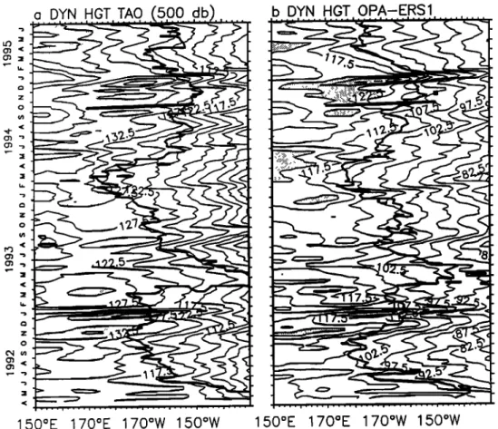
Figure
2. (a) Equatorial
section
of observed
Tropical
Ocean
Global
Atmosphere
(TOGA)-
Tropical
Atmosphere
Ocean
(TAO)
and
(b) OPA-European
Remote
Sensing
(ERS)-1
modeled
dynamic
heights.
These
dynamic
heights
are
referenced
to 500
dbar.
Areas
of pronounced
dynamic
height
pulses
are
shaded.
The
28øC
observed
isotherm
[Reynolds
and
Smith,
1994]
and
the
modeled
28øC
isotherm
are
superimposed
on
Figures
2a and 2b, respectively.
The FLUPAC
equatorial
transect
is superimposed
as a dark
line in
September-October
1994,
and
the
OLIPAC
cruise
is represented
by a dot
at150øW
in November
1994.
during
the fifth year. The model
was then forced
with the
1992-1995 dynamical simulation,
and results are then
examined from mid-April 1992 to June 30, 1995. From 15 ø to
20øS and 15 ø to 20øN the modeled nitrate is smoothly relaxed
to Levitus
climatology.
At the western
and eastern
boundaries
a similar
but stronger
relaxation
is imposed
in order
to remedy
abnormally
strong vertical advection
of nitrate due to
unrealistic vertical motions near America's and Papua New
Guinea's
coasts
in the dynamical
model. This procedure,
however, did not affect the dynamic or biological nitrate
fluxes at 165øE where the model results are compared to the
observations. The biological model is active down to 1260 m
depth
where nitrate
concentrations
are relaxed
to Levitus
climatology.3. Dynamical
and Biogeochemical
Fields-
Data and Model Comparisons
3.1. The Equatorial Pacific in 1992-1995
An equatorial section deduced from TOGA-TAO and
modeled dynamic heights (referenced to 500 dbar) is
presented
in Figure
2 together
with the observed
and modeled
28øC isotherm position for the period. The 28øC isotherm
position
is an indicator
of the position
of the eastern
edge
of
the warm
pool [Picaut
et al., 1996].
The equatorial
section
of
the modeled dynamic height (Figure 2b) shows a -10cm
systematic
mean
bias
with respect
to the observations
(Figure
2a). Reasons
for this are unclear
at present
and
merit
further
investigations.
However,
as in the observations,
time varying
features such as Kelvin pulses are in very good agreement.
The period
from 1991 to 1994 is characterized
by three
successive weak warm events that resulted in a long-lived
warm anomaly
in the equatorial
Pacific [Goddard and
Graham,
1997]. During that time the Southern
Oscillation
Index (SOI) remained
negative
[National Oceanic and
Atmospheric
Administration
(NOAA), 1994]. Kessler
and
McPhaden
[1995] described
the period 1991-1993
during
which
the U.S.-JGOFS
EqPac
cruises
took place.
Abnormally
high temperature
and low productivity
representative
of El
Nifio conditions
prevailed
during
the spring
cruise
as can be
seen here from the 28øC isotherm eastward positions (Figures
2a-2b).
In contrast,
the fall cruise
was conducted
when
near
normal conditions associated with a brief return of moderate
easterlies
were back [Murray et al., 1995] as indicated
by
28øC
positions
near
the dateline
both
in data
and
model.
From
October
up to December
1992, seasonal
occurrences
of
westerly
wind
bursts
were
observed
that are seen
both
in the
data and the model to generate downwelling Kelvin waves.
These
propagate
to the east
in association
with the warm
pool
eastward
displacement.
Then abnormally
warm conditions
3328 STOENS ET AL.: COUPLED PHYSICAL-NEW PRODUCTION SYSTEM
be more characteristic of a slightly enhanced seasonal cycle [Boulanger and Menkes, 1995]. After a brief retum of moderate conditions in late 1993 and the beginning of 1994, warm conditions returned during the last semester of 1994. This last semester of 1994 was characterized by a series of westerly wind bursts [Eldin et al., 1997]. The modeled variability is in very good agreement with the data both in terms of dynamic height and warm pool eastward displacement. During this time period the eastward shift of the warm pool was particularly pronounced, followed by a retreat of the warm pool position to the dateline during the first semester of 1995. This corresponded to weak cold conditions in the Pacific [Goddard and Graham, 1997].
These east-west oscillations of the eastern edge of the warm pool can be attributed to zonal advection by eastward currents [Picaut et al., 1996]. During the FLUPAC and OLIPAC cruises this resulted in positive SST anomalies as high as 2øC [NOAA, 1994] in the central Pacific in October- November 1994. Associated with the warm pool displacement and the series of westerly wind bursts, a series of downwelling Kelvin waves that may have further contributed to the eastward shift of the warm pool [Picaut and Delcroix,
1995] were generated in September, in November, and in December 1994 when the FLUPAC and OLIPAC cruises took place.
The first one was partly generated by a westerly burst near 160øE in early September [Eldin et al., 1997]. Following the September wave, a westerly wind event occurred in October [Eldin et al., 1997] at the beginning of the FLUPAC equatorial transect. This pulse, however, did not generate any
clear propagation of Kelvin wave signal in neither the TAO
dynamic height (Figure 2a), the TOPEX/POSEIDON sea level
anomaly (not shown), nor the model (Figure 2b). At that time
the zonal current observed by the TAO ADCP mooring
located at 165øE indicates westward flow down to a 100 m
depth. Hence the downwelling wave may have been damped by the interaction with the surrounding flow in opposite (westward) direction to the wave-induced eastward current [Brossier, 1987; McPhaden et al., 1986]. Another reason may be that a reinforcement of easterlies in the central Pacific, at that time, counteracted the genesis of the downwelling Kelvin wave. Then, in November, a marked westerly wind burst generated a clear downwelling Kelvin wave that propagated across the basin. The 'OLIPAC passage at the equator occurred while the Kelvin wave associated sea level was rising. Lastly, a strong westerly burst at the beginning of December 1994 forced a strong downwelling Kelvin wave and is observed propagating all the way to the eastern Pacific. It marks the end of Kelvin wave activity in the western Pacific (Figure 2) and of the eastward shift of the 28øC isotherm.
Remotely forced processes such as the downwelling Kelvin waves have been thought to affect the geochemical (nutrients) and biological (chlorophyll, primary production, plankton community structure) fields [Murray et al., 1994; Bidigare and Ondrusek, 1996]. They also contribute to the zonal displacement of the eastern edge of the warm pool. Thus the FLUPAC and OLIPAC cruises sampled the ocean during a period of time that appears to be affected by major features of the large scale equatorial dynamics which characterize the equatorial Pacific.
3.2. Vertical Physical and Biogeochemical Structures During FLUPAC and OLIPAC
3.2.1. Cruises data. The meridional FLUPAC transect at
165øE first sampled the tropical waters of the Coral Sea in the
south and then entered the warm pool waters (SST > 28øC) at
-10øS (Figure 3a). During this transect, conditions were close
to the reference conditions described in Radenac and Rodier
[ 1996]. The thermocline was rather diffuse as opposed to the
halocline (Figure 3b) which was well marked and shallower than the thermocline and decoupled from it. This decoupling was particularly apparent at 4øS-2øN where a low-salinity
core (<34.1 practical salinity unit (psu)), associated with the
westward flowing South Equatorial Current (SEC), was found
from the surface down to 100 m depth. At-•150 m depth, south of the equator, the high-salinity core (>34.9 psu) was characteristic of South Pacific waters of subtropical origin.
The Equatorial Undercurrent (EUC) was well developed with
a maximum
speed
of 50 cm s
'• at 175 m (Figure
3c). As is
often observed at this longitude, the surface mixed layer was
nitrate-exhausted all along this transect down to -75 m, including the region close to the equator (Figure 3d). The nutricline closely followed the halocline, and the subsurface
chlorophyll
maximum
(Figure 3e) that peaked
at 0.5 I.
tg L 't
was found at the nutricline depth as is commonly observed. During the OLIPAC cruise the isotherms near the equator at 150øW showed the characteristic spreading indicating the presence of the EUC core at 150 m depth (Figures 4a and 4c).
They slowly and gradually spread and deepened to the south
as was previously described during the Hawaii-Tahiti shuttle
experiment [Wyrtki and Kilonsky, 1984]. Around 150 m the
high-salinity tongue originating from South Pacific
subtropical waters (Figure 4b) penetrated from the south
toward the equator. The core of the EUC had a maximum
velocity
of 70 cm s
-• (Figure
4c). Above
it the flow remained
eastward almost up to the surface. Farther south, currents
were weak and mostly westward except around 10øS where
an eastward flow was measured, as is occasionally reported in the central Pacific [Eldin, 1983; Wyrtki and Kilonsky, 1984; Kessler and Taft, 1987]. The observed distribution of nitrate (Figure 4d) was close to those previously described in the central Pacific [Carr et al., 1992; Wyrtki and Kilonsky, 1984; Murray et al., 1995]. The mixed layer was nutrient depleted south of 10øS. To the north, surface concentrations were similar to the values observed during the 1992 spring EqPac cruise characteristic of E1 Nifio warm conditions [Murray et al., 1994]. Correspondil•g to this nitrate structure, the chlorophyll distribution showed a deep chlorophyll maximum below the top of the thermocline in the southern part of the section and showed relatively high chlorophyll values
(>0.25 gg L '•) extending
from 100 m up to the surface
to the
north (Figure 4e). This transition from an oligotrophic regime to a mesotrophic one has been previously described in the area between 130 ø and 140øW, where its latitude varied between 10 ø and 14øS [ Dandonneau and Eldin, 1987].
Both at depth and at the surface the equatorial FLUPAC transect sampled two different physical regimes which are
more extensively described by Eldin et al. [1997]. The
boundary between these two regimes is best evidenced in Figure 5b which shows a sharp salinity front of--0.8 psu near
STOENS ET AL.' COUPLED PHYSICAL-NEW PRODUCTION SYSTEM 3329 5O 100 150 200 50 100 150 200 0 ,.• 50 E ..c 100 m 150 200 50 lOO 150 2OO
FLUPAC 165øE MODEL 165øE
b.s91!n!ty
'
g salinity,
c zonal velocity
,
,
h zonal velocity ,
,•
':':':':'•'
.:_:.:.
•..-,...•.•.:.::.:....:.•.
, .:•::.:•
....
•-:::•:•
'::::
....
... ! ...
nitrate , , . ! .... i .... i .... -% t %,,.1 i nitrate i i ! ! i i i ,,•-•--.. 0.15"-.--• 1.•---0.20 ..-. 50 ... ' ...m
150
200o.••
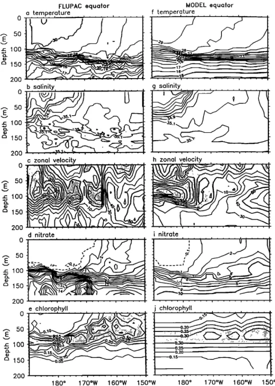
15oS 100S 5øS 0 ø SON 15øS 10øS 5øS 0 ø 5øNFigure
3. (a)
Temperature
(øC),
(b)
salinity
(•ractical
salinity
unit
(psu)),
(c)
zonal
velocity
(cm
s-•),
(d)
nitrate
(lamole
kg-•),
and
(e) chlorophyll
(lag
L' ) observed
during
FLUPAC
along
165øE
and
(f-j) simulated
by the OPA-ERS-1
model.
Westward
currents
are shaded.
175øW. The fresh (<35 psu) and warm (29ø-30øC) waters
west of this front were characteristic of the warm pool waters
with a salinity
barrier
layer
above
the thermocline
[Lukas
and
Lindstrom,
1991], representing
the continuity
at depth
of the
east-west surface front. A well-marked thermocline was located between 100 and 125 m all along this transect (Figure5a), and the absence of an east-west slope was characteristic
of El Nifio conditions [Philander, 1989]. The surface current
(Figure
5c) showed
a dominantly
westward
SEC except
in the
eastern
part of the transect
where
the westward
flowing SEC
usually
prevails
[Wyrtki
and Kilonsky,
1984;
Kessler
and Taft,
1987; Eldin et al., 1997]. Nevertheless, surface current
reversal has been commonly observed at this longitude, in
springtime,
during
El Nifio periods
and/or
associated
with
downwelling
Kelvin waves
[Firing et al., 1983; Kessler
and
3330 STOENS ET AL.: COUPLED PHYSICAL-NEW PRODUCTION SYSTEM
near 175øW, was probably associated with the October westerly wind event [Eldin et al., 1997]. At subsurface a strong westward current was situated fight above the thermacline in the west. This type of structure, already observed west of the salinity front, has been interpreted as the response to a westerly wind forcing [Kuroda and McPhaden,
1993]. It can also be indicative of the dynamics associated with subduction of the SEC under the salinity barrier layer as explained by Yialard and Delecluse [ 1998a, b]. The EUC was located beneath and tilted upward toward the east. The distribution of chlorophyll concentration was consistent with the salinity distribution (Figure 5e): the salinity front
separated chlorophyll poor waters in the warm pool from
upwelling waters where chlorophyll was more abundant. At first sight this front similarly separated nitrate-exhausted
water of the warm pool from the nutrient rich upwelling region (Figure 5d). However, one can note a spatial offset
between
nitrate-exhausted
waters
([NO3]<0.1
ginale
kg
4) and
the salinity or chlorophyll front ([Chl]<0.1
ggL 4) or
zooplankton front (Figure 1). This offset was most probably controlled by biological processes in which nutrient removal
by phytoplankton exhausted the nitrate dynamical supply near
the barder layer. The nitrate concentration increased eastward,
reaching
values
>3 ginale
kg
'l at 150øW. In the upwelled
waters, consistent with the availability of nitrate in the upper
well-lighted waters, the chlorophyll maximum was located in
0 lOO 15o 200 250 ,300 0 lOO 15o 200 250 ,300 01,.11 150øW
•roture f tem erature MODEL 150øW
!
zon velocit'
,c , ,al, . . y ... ß - - • - ß Y- ß ! - - h zonal velocit' i
o • . 0 lOO 15o 200 25O 3O0 d nitrat9 i nitrate
... ' ...
e
chloro
h
I•
j chlorophyll
::;:i:;:i:.:: :;: :;:;:L .:•i• •i.::.!.•.t• ...:::.•;•:•]::•:.!•?:!•!;;•!::!::!;!•::!?.?.;•!!:.?•!•!:::::::::::::::::::::::::
...
:::::::::::::::::::::::::::::::::::::::::::::::::::::::::::::::::::::::::::::::::::::::::::::
lOOS 5øs o o ! 1 oøs 5øS o o o lOO 150 200 25O 300STOENS ET AL.' COUPLED PHYSICAL-NEW PRODUCTION SYSTEM 3331 5O 100 150 200 FLUPAC equator a temperature ß , , MODEL equator
f ,te,m,pe,
ra,
t .u
r.e ...
.... ! ß - ß ; ! • ß ß
b salinity
g.s.ali.ni!y,
.
0
13
....
.--. 50 • lOO r• 150 200 . 0 • 100 r• 150 200 ... • 50 E z: 100 r• 150 200 nitrate. . . i .... •1...
•'jI
' ' ' ! .... i
'5---- ,;- .zo.,-[i
0
nitrate .... i .... i .... i .... , ,11 j chlorophyll O .... ! , i i .... ... 0•25 ... "' ... ' ... " ß....
150200 ...
:::: ...
o 70ow soow soow o 70.w
Figure 5. Same
as Figure
3 but for the FLUPAC
equatorial
section.
the surface mixed layer. On the warm pool side a deep (80 m)
chlorophyll maximum was positioned just below the salinity
barrier layer at the top of the nutricline. The chlorophyll
concentration
in the deep
maximum
was
4).30 I•g L-I and
was
similar to that found in the upwelled waters farther east. In
terms of biomass per square meter, however, the upwelled
waters were richer than the warm pool waters because the
chlorophyll rich layer was thicker there (see also section 4).
Hence the FLUPAC equatorial data highlighted one of the
most remarkable features of the equatorial Pacific: the warm,
fresh, and oligotrophic waters of the westem Pacific warm
pool are separated by a sharp salinity front from the colder,
saltier, and mesotrophic waters of the upwelling waters. These
two contrasted regimes are also evidenced in the upper
trophic levels such as zooplankton distribution (Figure 1).
3.2.2. Model results. At 165øE, modeled temperatures are
generally
in good
agreement
with the data at the same
depth
(Figure 30. However, the model temperature
shows less
spatial
structure
than the data, and in particular,
it fails to
reproduce
the spreading
of isotherms
in the core of the EUC.
The fresher water (<34.1 psu) in the equatorial region is
correctly
simulated
although
the surface
front south
of 4øS is
more intense than in the observations (Figure 3g). The modeled EUC is much weaker than the observed (Figure 3h).
3332 STOENS ET AL.: COUPLED PHYSICAL-NEW PRODUCTION SYSTEM
This discrepancy explains the lack of spreading of the isotherms in the modeled temperature. It has to be noted that the modeled current structures are much simpler than the observed and that countercurrents are generally too weak in this simulation.
At 150øW, thermohaline structures are generally well reproduced, but there are systematic biases such as colder temperatures in the upper layers and fresher waters in the salinity field. Zonal velocity shows patterns that are too smoothed (Figures 4c-4h) as compared to data and do not
present any current variability south of 5øS. It has also to be
stressed that the EUC core is too shallow.
In contrast, the equatorial transect is quite well simulated. The temperature distribution is good despite a 1 øC bias in the upper layer waters (Figure 50. The salinity field (Figure 5g) is well simulated. In particular, the salinity zonal gradient and its location are well reproduced. Being able to correctly simulate this gradient is crucial as it was seen to separate two different regimes. In the western part of the equatorial transect the EUC is weaker in the model than in the data and tilts upward toward the east where both data and model agree better (Figure 5h).
Considerations about dynamical simulations of these three particular transects are consistent with the more general conclusions of Grirna et al. [1998]: the EUC core and the thermocline depth are shallower in the model than in the data, and the thermocline is generally too diffuse (as most modeled thermocline) and the countercurrents are too weak in the model.
In the oligotrophic region (warm pool), at 165øE, the surface NO3 depletion (Figure 3i) is deeper than the observed and the nutricline tends to be too diffuse compared to observations. This can drive significant differences between
observations and model outputs below the mixed layer.
Reasons for this are certainly various. Among those the
tendency of the model to have a too diffuse pycnocline
structure can be invoked, as the nutricline is, at first order,
shaped by the pycnocline structure in observations [Radenac
and Rodier, 1996]. Discrepancies between the data and model due to limitations of the biological nitrate sink will be evoked later in the text.
At 150øW, the upper layer NO3 concentrations are reasonable, and the transition between nutrient poor
([NO•]<0.1
gmole
kg
-•) and nutrient
rich waters
is fairly well
reproduced (Figure 4i). At depth, obvious biases show up
such as a too shallow nutricline. It is hard to understand what factors control these biases in such complex 3-D dynamics. However, some of the spurious nutrient trapping near the surface may be related to the lack of horizontal transport of organic nitrogen as evoked in the model description [Najjar et al., 1992; Bacastow and Maier-Reimer, 1991]. In the equatorial region the simulated nitracline shows a weaker than observed doming associated with the EUC core. This lack of
structure is obviously related to the simulated EUC that is too
shallow compared to the data (Figures 4c-4h).
Along the equator the surface transition between nutrient poor (oligotrophic) and nutrient rich (mesotrophic) waters is correctly simulated (Figure 5i). In the model this surface transition in the nitrate field is totally correlated to the salinity front at that period of time (see section 4). Therefore, if the
offset seen in the data between the salinity front and nitrate-
exhausted waters is indeed related to biological activity, our
simple nitrate sink model does not reproduce this process. At
depth, however, this transition is found at the bottom of the
barrier layer, as in the data, which indicates that processes
maintaining the depth of the poor pool differ from those
maintaining the barter layer. Underneath the photic layer the
nutricline is too diffuse compared to the data.
The chlorophyll values, which are statistically computed in
the model, show higher surface concentrations and a much
smoother pattern than are in the observations (Figures 3j, 4j,
and 5j). This is not surprising as the statistics used here have
been derived globally and thus cannot account for local
variations as observed along the transcot. The position and
values of the deep maximum chlorophyll are rather well
captured by the statistics. In the mesotrophic region, modeled
chlorophyll is generally 30%-40% too high compared to
observations but the deep chlorophyll maximum is well
located (Figures 4j and 5j).
The validations of the coupled dynamical-biogeochemical conditions along the FLUPAC and OLIPAC transects have shown that despite imperfections the model is able to
reproduce the major observed features at specific locations
and times with good qualitative agreement. In particular, one
important aspect and one merit of these simulations are that they are able to reproduce the two contrasted regimes of the equatorial waters.
4. The Modeled New Production
4.1. Modeled New Production at the Equator From 1992 to 1995
The variability of temperature and salinity distributions,
currents, and dynamic topography of the model outputs is in
good agreement with TAO buoy observations over 1992-1995
(see above and Grima et al., [1998]), and the modeled nitrate
field is also reasonable
compared
to the observations
(see
above). This allows us to investigate further the large-scale
equatorial features of coupled conditions during 1992-1995 as
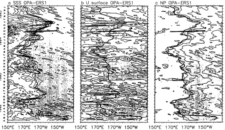
given by the simulations. Figure 6 shows the equatorial
section of modeled sea surface salinity (SSS), zonal currents, and new production. The succession of westward and eastward zonal currents is responsible for the zonal displacement of the eastern edge of the warm pool and fresh pool (SSS<34.8 psu). The mechanisms creating these east-
west migrations are detailed by Picaut et al. [1996] and by
Delcroix and Picaut [1998]. Thus the warm/fresh/poor pool region is moved east and west according to the large-scale ENSO-related zonal current.
In this model output ('Figure 6) the well-marked salinity front (Figure 6a) that separates the fresh warm pool to the west from the upwelling region moves eastward and westward
and is displaced by the zonal currents (Figure 6b). Strong
pulses of eastward velocities are shown to be associated with the occurrences of downwelling Kelvin waves such as those of November-December 1992 and 1994. The SSS front is
seen to be particularly pronounced during these events when
current convergence at the front is particularly strong. The last
semester of 1994 is the longest period when the zonal current
is mostly eastward. This causes the front and the eastern edge
of the warm pool (position of the 28øC isotherm) to gradually
move eastward and to sharpen. When eastward currents are not so strong or westward currents occur, the salinity front is
STOENS ET AL.: COUPLED PHYSICAL-NEW PRODUCTION SYSTEM 3333
more diffuse (Figures 6a and 6b) [Vialard and Delecluse, 1998a, b].
Primary production allows us to differentiate between the equatorial poor and rich regimes (Figure 6c). Figure 6c clearly shows that during the 1992-1995 period, two distinct regimes prevailed that are characteristic of the warm pool (poor pool)
region on one side and the upwelling region where waters are
richer on the other side. These two regimes are separated by a "primary production front" that is closely related to the salinity front (see the position of the 34.8 psu isohaline and the primary production front on Figure 6c). Only during the first three months of the simulation, a decoupling between the new production and salinity front occurs. This time period should be considered with caution in the simulation as it is close to the ending of the 5 year spin up calculated with a perpetual April 1992 to March 1993 year. Note that the relation between the primary production front and the eastern edge of the warm pool is particularly strong when the salinity front is well marked, in November-December 1992 and during the last semester of 1994, and closely follows the displacements of the salinity front. The FLUPAC and OLIPAC cruises sampled this last episode.
As seen in Figure 5, observed nitrates at the time of FLUPAC closely reflect the position of the simulated primary production (nitrate) front which is therefore displaced via zonal advection during the period of interest. Additional data from November-December 1994 [Inoue et al., 1996] show that the modeled front position is also in agreement with observations at that time. The variables recorded along the
equator during FLUPAC further confirm that the front actually separates the oligotrophic warm pool region from a mesotrophic regime east of the front (Figure l).
Consequently, primary production can vary greatly during El
Nifio or La Nifia periods because of these large east-west displacement patterns of the warm pool. For example, it was greatly reduced during late spring of 1992, at 140øW, in agreement with the observations made during the EqPae
spring cruises [Murray et al., 1995]. However, further
simulations of the ENSO cycle are required to really estimate
primary production reduction when strong El Nifio occurs. In
particular, spectacular impacts of the 1997-1998 El Nifio
should give further insights on such reductions.
4.2. Comparison Between the Warm Pool and the Upwelling Regimes
Given the clear separation between the regimes, it is useful to introduce the NINO4 (160øE-150øW, 5øS-5øN) and NINO3 (150ø-90øW, 5øS-5øN) boxes often used to contrast two dynamical (warm pool and upwelling) regions for ENSO-
related
issues
[NOAA,
19'94].
Indeed,
during
the 1992-1995
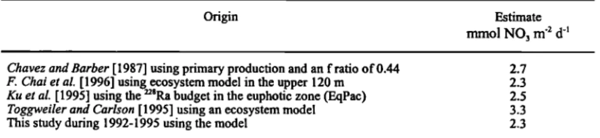
time period one can see that these two regions correspond to the warm pool region (NINO4) and the upwelling region (NINO3). Averaged primary production amounts to -0.9
mmol
NO3
m -2 d 'l in NINO4 and 2.1 mmol
NO3 m '2 d 'l in
NINO3. These can be thought of as representative of mean conditions during this weak ENSO period for the two regimes. o SSS OPA-ERS1 ,-. z o z o z o •50øE •70øE •70øW •50øW b U surfoce OPA-ERS1 150øE 170øE 170øW 150øW c NP OPA-ERS1 150øE 170øE 170øW 150øW
Figure 6. OPA-ERS-1 model outputs along the equator for the whole simulation: (a) salinity (psu), (b) zonal
1
velocity
component
(cm s' ), (c) new production
(mmol
NO3 m '2 d-'). Sea Surface
Salinity
(SSS) > 34.8 psu,
westward
currents,
and
new production
> 1 mmol
NO3
m '2 d 4 are shaded.
The 34.8 psu isohaline
marking
the
SSS front is superimposed on Figures 6a-6c. The FLUPAC equatorial transect is superimposed as a dark line