A simplified energy model for analysis of building envelope thermal characteristics

READ THESE TERMS AND CONDITIONS CAREFULLY BEFORE USING THIS WEBSITE. https://nrc-publications.canada.ca/eng/copyright

Vous avez des questions? Nous pouvons vous aider. Pour communiquer directement avec un auteur, consultez la

première page de la revue dans laquelle son article a été publié afin de trouver ses coordonnées. Si vous n’arrivez pas à les repérer, communiquez avec nous à PublicationsArchive-ArchivesPublications@nrc-cnrc.gc.ca.

Questions? Contact the NRC Publications Archive team at

PublicationsArchive-ArchivesPublications@nrc-cnrc.gc.ca. If you wish to email the authors directly, please see the first page of the publication for their contact information.

NRC Publications Archive

Archives des publications du CNRC

This publication could be one of several versions: author’s original, accepted manuscript or the publisher’s version. / La version de cette publication peut être l’une des suivantes : la version prépublication de l’auteur, la version acceptée du manuscrit ou la version de l’éditeur.

Access and use of this website and the material on it are subject to the Terms and Conditions set forth at

A simplified energy model for analysis of building envelope thermal

characteristics

Cornick, S. M.; Sander, D. M.

https://publications-cnrc.canada.ca/fra/droits

L’accès à ce site Web et l’utilisation de son contenu sont assujettis aux conditions présentées dans le site LISEZ CES CONDITIONS ATTENTIVEMENT AVANT D’UTILISER CE SITE WEB.

NRC Publications Record / Notice d'Archives des publications de CNRC:

https://nrc-publications.canada.ca/eng/view/object/?id=a09dd9e5-93a6-4b2a-918c-0adac2d0bc76 https://publications-cnrc.canada.ca/fra/voir/objet/?id=a09dd9e5-93a6-4b2a-918c-0adac2d0bc76

Sleven M. CornickandDaniel M. Sanderare research officers at the Building Performance Laboratory of the Institute for Research In Construction, National Research Council of Canada, Ottawa, ON.

A SIMPLIFIED ENERGY MODEL FOR

ANALYSIS OF BUILDING ENVELOPE

THERMAL CHARACTERISTICS

ABSTRACT

687 Energy Code for Buildings. For example, Crawley (1992) describes why methods such as ASHRAE Stan-dard 90.1 were not appropriate for Canadian climates. The 'gain-Ioad method developed by Sander and Bar-akat (1983), (1984) did not combine the effects of solar and internal gains and was developed for houses. A new method was required.

The simple energy model described here consists of equations to predict the heating- and cooling-system loads, per m2_{of gross wall, as a function of orientation,}

climate, internal loads, and wall/window characteris-tics. The system loads, sometimes referred to as "coil loads," represent the heating and cooling energy that is provided by the heating, ventilating, and air-condition-ing (HVAC) system; they do not include heatair-condition-ing system efficiency or cooling coefficient of performance (COP). These are accounted for separately so that the equations are not dependent on the energy source (fuel).

The modelfor heating consists oftwo parts:

• the heat-loss term, whichisa linear function ofD, with the slope and intercept dependent on climate; and • modifier terms, which are functions ofV and W, that

reduce heating to accountfor solar and internal gains.

Thecooling model issimilar. In this case, the two parts are a base cooling term, whichisa linear function of parame-tersVandW;and a modifier term, which adjusts the cooling as afunction ofheat loss parameter,U.

These simple models produce annual values for heating and cooling energy that are within 10% of those from the DOE-2.1E runs for a wide range ofparameters.

This method for predicting energy use was used in the life-cycle cost-analysis procedure to determine prescriptive re-quirements for the energy code. It also forms the basis for trade-off procedures that can be used to demonstrate compli-ance for alternative combinations of envelope characteristics that deviate from the prescriptive requirements.

Daniel M. Sander

Thermal Envelopes VIIBuilding Energy Codes-Principles

Steven M. Cornick

A new National Energy Code for Buildings has been devel-oped in Canada. For this newcode, a simplified model was developed to estimate the change in energy consumption asso-ciated with a change in envelope thermal characteristics. This energy model was derived from a set ofcorrelations based on a large number (more than 5,000) of DOE-2.1E simulations for 25 Canadian locations. These correlations predict heating and cooling energy based on location and building envelope char-acteristics and internal gains from people, lights, and equip-ment.

This paper describes the design of the correlation equa-tions, compares the results of correlation equations with DOE-2.1E simulation results, and briefly discusses how the energy-correlation model was used in thenewenergy code.

The simplified model represents a building by three basic parameters:

-heat loss parameter,D;

-solar gain parameter,V;and -internal gain parameter,W.

The development of a new Canadian energy code (NRCC 1994) required a simple, fast means of calculating the change in heating and cooling energy that would re-sult from a change in building envelope characteristics. This was needed for the life-cycle costing analysis that was employed for choosing the prescriptive envelope re-quirements for the code. The basis of such an analysis is to minimize the sum of incremental construction cost and the present value of incremental energy cost. This proce-dure is described in a companion paper (Sander et al. 1995). The simple energy model also is used in the "trade-off compliance" option (Sander and Cornick 1994), which permits deviation from some of the prescriptive require-ments provided others are exceeded, such that the result-ing energy performance is "equivalent" to prescriptive.

Other simplified correlation-based energy models exist, but they were not appropriate for the Canadian INTRODUCTION

(2) 2 (MIlm .yr) (1) 2 (MIlm .yr) Q = L·SGRF·IGRF·GIF

TABLE 1 LCoelficlenls lor OIIawa

Easl Wesl North South

q, 728.8679 722.127 721.3787 729.1496

b, 431.2615 444.9293 463.3301 421.1035

iJ

parameter(W/m2_•K),

constant representing infiltration and ventila-tion losses(W/m2 .K), and

relationship between V-factor and heat loss (K). The annual heat loss was found to be only slightly de-pendent on orientation. The coefficients b

_o

and b₁vary only by a few percent for different orientations, indicat-ing that solar radiation on the wall surfaces is not a major factor. As expected, values of coefficients b

_o

and b₁are dependent on location. The coefficients for Ottawa

are

shown in Table 1.

where

U =

b

_o

=

b₁ =

whereL, SGRF,IGRF, and GIF are as defined below. The relationship between the annual heating system load, Q, and the three parameters, U, V, and W, was derived for one 10cation-0ttawa, Ontario. Once a plausible model was found, it was tested using other selected locations chosen to reflect the climatic variation across Canada. The proposed model predicted the annual heating system loads accurately for the other locations. In the final model, the annual heating system load, Q, was calculated by modifying the annual heat loss,L, by factors to account for solar and internal gains (Equation 1). This model takes a similar approach to that proposed by Sander and Barakat (1984) and accounts for the interaction of solar and internal gains. A more complete description is given by Cornick and Sander (1994).

HEATING ENERGY EQUATIONS

= floor area associated with envelope, typically 4.5 m (15ft)deep (m2_);

= opaque wall V-factor(W/m2_·K);

= window V-factor, including frame(W/m2_·K);

= window shading coefficient (dimensionless); and

= design heat gain from lights, people, and equip-ment(W/m2_{floor area).}

Annual Heat Loss,

L

The authors began by examining the annual heat loss, L,the heating when there are no internal or solar gains. L can be approximated as a linear function of U as

dimensionless

U =

IA..

_{Ug+A w' Uwl/A,} V = A_{g .}SCglA,

W = I.A/A, where

Au, = opaque wall area (m2);

A_g = window wall area including frame (m2); A, = gross wall area,(Au, +A_g)(m2); '"

ASSUMPTIONS

688 Thermal Envelapes VI! Building Energy Codes-Principles

The simple energy model was derived from a data base of 5,400 DOE-2.1E simulations for 25 Canadian locations (Crawley 1992). Four exterior zones facing the cardinal orientations were modeled. Each perimeter zone comprised a lightweight exterior wall having a layer of insulation of unit thickness and variable V-value, as well as a strip of glazing running the entire length of the wall, a medium-weight concrete floor, lqId adiabatic interior walls (Cornick and Sander 1995). The transient response of the envelope was calculated by DOE-2.1E. The following assumptions were made:

• no interzonal heat transfer,

• fixed infiltration rate of 0.25 L/s·m2(0.05 cfm/ftZ), • internal loads on a six-day office-type schedule, • heating setback to 15°C (59°F) and cooling off when

unoccupied,

• variable-air-volume (VAV) system with terminal re-heat,

• 13°C (55°F) supply air,

• free cooling (enthalpy-controlled air-side econo-mizer), and

• minimum ventilation as prescribed by ANSI/ASH-RAE 62-1989 (ASHANSI/ASH-RAE 1989) requirements-9.4 L/s'person (20 dm/person).

The building envelope was characterized by three parameters: a transmission parameter, U, which accounts for the heat loss or gain through the envelope; a solar parameter,V, which accounts for the solar gain through the envelope; and an internal-gainｰ ｡ ｲ ｡ｭ･ ｴ ･ W,which accounts for internal load.

The parameters are defined as

Because the energy-eode analysis was restricted to a relatively small number of Canadian locations, the authors began by producing coefficients that were loca-tion specific for those regions for which analysis was to be done. Later, the authors found it was possible to extend the application of the model by correlating the coefficients to climate parameters.

This paper describes the design of the correlation equations, compares the results of correlation equations with DOE-21E simulation results, and briefly discusses how the energy-eorrelation model was used in the new energy code.

(7) (5)

(6) Q = L·SGRF·IGRF

GIF = Q(from DOE2.IE) / (L· SGRF . IGRF)

689

where

1This constraint was derived from the following boundary condition:ifSGRF or IGRF has a value of 1 then there is no interaction,'Ybecomes 1 and the value of GIF becomes1. Con-sequently; the sum of the coefficients must beO.The "or" here is inclusive.

'Y = (1 - SGRF· IGRF)

I

«1 - SGRF)+(1 - IGRF))

'Y = 1 if SGRF and IGRF=1.

Several things were apparent from a plot of GIF vs.'Y.

First, the gain interaction factor, GIF, was not dependent on orientation. Second, GIF was not strongly dependent on lOCation. Consequently, a universal curve was fitted for GIF vs.'Yusing all the orientations for all the selected locations. The result was a single correction term for all Canadian locations (Equation7).The coefficients for the GIF are given in Table 4.

'Y = total gains/(solar gains+internal gains)

'Y = (L - Q)I «L - Lv)+ (L - _Lw))

'Y = (1-QIL) I «1-LvIL)+(1-LwIL))

However,4/L=SGRF,Lw/L=IGRF, andQIL=SGRF ·IGRF; therefore,

Another parameter,'Y,was defined. This is the ratio of total gains (L- Q)to the sum of solar gains (L- Lv)

and internal gains(L- Lw)'

When solar and internal gains are present, it was found that the annual heating system load, Q, could be approximated by the product of the annual heat loss, L, and the solar and internal gain reduction factors, SGRF and IGRF, respectively (Equation 5).

Solar Gain and Internal Gain

Interaction Factor, GIF

However, to improve the accuracy of the results with both internal and solar gains interacting, an additional factor, the gain interaction factor (GIF), was introduced. GIF was introduced to account for solar and internal gain interaction and was defined as the ratio of Q obtained from DOE-2.1E to the product of L, SGRF, and IGRF calculated from the simulation results (Equation 6).

(4) All Orientaflons ｾ -15.6865 ｾ 2.002871 ｾ -593,541 = WIL.

TABLE3 IGRF Coefficients for Ollawa y

Internal Gain Reduction Factor, IGRF

Internal loads also reduce the annual heating loss for a building. The annual heating loss minus the internal gains was defined as L_w(Le., L - internal gains). When L_w was plotted with the internal gain parameter, W; the six different curves, representing the values of the U param-eter, were again apparent. In a similar manner to solar gains when both Lwand W were divided by the annual

heat loss, L, all the curves collapsed into one. Fitting the curve obtained by plottingLwlLagainst WILproduced a single equation (Equation 4) that suited the 25 data-base locations. However, because the effect of internal gains on heating was independent of orientation, a sin-gle set of coefficients resulted for a given location. Table 3 shows the coefficients

131, 132,

and

133

for the Ottawa location.

where

where

Thermal EnvelopesVIIBuilding Energy Codes-Principles

x = VIL.

TABLE 2 SGRF Coefficlenfs for Ollawa

East West North South

"1 2528,154 2436.595 1396,895 3344,05 lXz -896615 -873968 -274133 3672654

"3 1.44E+09 1.48E+09 3.36E+08 1,6E+09

Solar-Gain Reduction Factor, SGRF

Next, the authors examined the reduction in heating due to solar gains.Lvwas defined as the annual heating loss minus the solar gains (i.e., L - solar gains). A plot of Lvagainst the solar gain parameterVrevealed six differ-ent curves, each represdiffer-enting a particular value of U. However, dividing both

4

and V by the annual heat loss L accounted for the effect of U and the six curves col-lapsed into a single curve.

The authors defined the ratio

41

L to be the solar-gain reduction factor (SGRF). Fitting the curve of LviL against VIL produced a single equation (Equation 3) that suited all 25 data-base locations. Four sets of coeffi-cients, one for each orientation, were produced for each location in the data base. Table 2 lists the coefficients av

llz,andllJobtained for Ottawa.

2 3

East Wes! North South C_min

Thermal EnvelapesVII Building Energy Codes-Principles

2For warmer climates, such as Australia, the envelope effect was found to be much less and,in some cases, was opposite for hot locations such as Darwin, Australia.

3Infact, several weather stations were selectedby the provin-cial ministries for the Energy Code that were not amongthe listoflocations simulated. The climate correlations were used

to generate the coefficients for the heating and cooling equa-tions that subsequently appeared in the life-cycle costing anal-ysis procedure and trade-off specification (Sander and Cornick 1994).

Cooling

Because the climate correlations for cooling are more straightforward, they will be presented first. There are five coefficients in Equations 8, 9, and 10 that need to be deternlined. They are

ao = intercept for the base cooling load,

aj = variation of cooling with solar parameter, a2 = variation of cooling with intemalload parameter,

ｾ = variation of cooling with thermal transmittance, and

The heating and cooling equations were derived with location-specific coefficients for the 25 Canadian lo-cations. To permit calculation for Canadian locations not in the original data base, the method was extended so that heating and cooling loads could be predicted from basic climatic data such as heating degree-days, cooling degree-days, and the amount of solar radiation.3 Cor-nick and Sander (994) give a more complete description of the derivation of the climate correlations for the heat-ing and coolheat-ing equations.

2

l>C

_o

=

a

_{3 . U·} (1-CminlC

_o)

(MJjm .yr) (10)

CLIMATE CORRELATIONS

Correction for Envelope Losses/Gains,

ｾ ｃ

The effect of the U parameter on cooling was accounted for by applying an envelope correction term to the base cooling load,Co'Incooler climates, such as Canada, building envelopes tend to experience net transmission loss. The DOE-2.1E simulations showed that as U increased, more heat was lost through the envelope and the annual cooling system load decreased. This was, in effect,free cooling obtained by increasing the envelope transmission. However, this free cooling was obtained at the cost of a substantial increase in the heating load in Canadian climates.2

The envelope correction term,l>C

_o,

was defined as the change in cooling system load given a change inU from U= 0 to U= U while holdingV and W constant (Equation10).Envelope transmission losses for cooling tend to be relatively small when compared to the base cooling load. The coefficienta3from Equation 10 alsois climate and orientation dependent. Table 5 shows the values of thea3coefficient for Ottawa.

(8) 2 (MJ/m .yr) "0 22.0343 24.824 15.103 19.473 87.684 a, 857.662 816.929 506.308 789.254 02 4.076 4.111 4.175 4.115 03 -41.259 -46.518 -52.063 -43.619 .ｾ 690

whereCo andl>C

_o

are as defined below.

Base Cooling Load,

Co

The authors began by examining how the cooling loads vary with changes in solar and internal gain. When U was held constant, the cooling load varied in direct proportion to the solar gain and internal gain parametersVand W However, the cooling loads did not go below a minimum value,_Cmiweven for combinations of U, V, and W that produce little to no cooling load. This minimum cooling was a result of the choice of system modeled and the operational assumptions, especially the minimum ventilation requirement. The value of_Cmin was found to be climate dependent. The base cooling load,Co' was defined as:

2

Co= max_(Cmin>ao+a

j •V+a2.W) (MJ/m .yr) (9)

where

Cmin =minimum cooling load for a particular climatic location and

ao, avanda2 = climate- and orientation-dependent coef-ficients.

Table 5 shows the values of the coefficients for Ottawa. TABLE5 Cooling Coelllclenls lor Ollawa TABLE4 GIF Coelficlenls (The Coelficlenls Are

Independent 01 Locallon and Orienlallon)

COOLING ENERGY EQUATIONS

a,

-7.631

a,

24.608

a

₃ -26.340

a

4 9.3629

The relationship between annual cooling system loads and the three parametersU, V, and Wwas derived in a manner similar to that for heating. Annual cooling system loads, C, primarily are dependent on internal and solar gains rather than envelope losses. A simple two-step model was derived to estimate cooling system loads (Equation8). First, the base cooling load, Co,is cal-culated from the internal gain and solar gain parameters V andWThen the base cooling loadiscorrected for the envelope transmission parameterU. A detailed descrip-tion of the derivadescrip-tion of the cooling equadescrip-tionsis given by Sander et al. (1993) and Cornick and Sander (1994).

Thermal Envelopes VIIBuilding Energy Codes-Principles

e

min = minimum cooling load.

(16) (17)

b

_o

= _{AD +Al .}HDD65

b

_o

= B

_o

+_{Bl .}HDD65

TABLE 7 Climate Correlations lorL

East West North South

Ao 176.797 169.889 173,548 170,561

A, 0.0609 0.0612 0,0608 0,0615

Bo

106.531 111.498 131.917 97.449 B, 0.0379 0.0382 0.0378 0.0376

691

The coefficientsE, L, G,T, andX for the climate correla-tions are shown in Table 6.

Table 7 shows the climate coefficientsA and Bfor pre-dicting the annual heat loss coefficients.

Solar Galn Reduction Factor The coefficients for the solar gain reduction factor (SGRF) (Equation 3) were determined by a simple best fit; the authors have not tried to ascribe physical significance to the coefficients. The sign of the higher order coefficients changed de-pending on the data, making it difficult to correlate them to climate. Therefore, a different approach had to be used. Instead of generating climate correlations for the coefficients in Equation 3, the entire curve defining SGRF was modified to coincide with a reference curve. To calculate SGRF for a location not in the original data base new coefficients are calculated by modifying the coefficients of the reference location for the effects of cli-mate. A climate factor, k_{l ,} was generated to modify the SGRF coefficients for Ottawa, the reference location.

Figure 1a shows the curves for the SGRF for Ottawa and Vancouver (east orientation). The curves have the same general shape.Ifthe curve for Vancouver is shifted along the independent axis it is possible to calculate the SGRF for Vancouver using the curve derived for Ot-tawa. To do this, the value of VI L for Vancouver is mod-ified by an amount, k

_v

such that the values of k_{l ·}VI L

and V IL correspond to the same SGRF on the Ottawa Heating

The first step in developing climate correlations for the heating coefficients involved finding a correlation for the annual heat loss, L. The next step involved pre-dicting the solar and internal gain reduction factors for a specific location. The gain interaction parameter was found to be independent of climate.

Annual Heat Loss Like the cooling equations, the coefficients b

_o

and b_lhave some physical significance; b

_o

accounted for the infiltration and ventilation losses, while b_l characterized the effect of thermal envelope transmission on the heating requirement for a given cli-mate. As may be expected, the coefficients b

_o

and b

_v

whichareused to calculate the annual heat loss (Equa-tion 1), were found to be linearly related to heating degree-days (Equations 16 and 17).

South -10,859 0.0686 0.0152 0.0177 -1.8E-05 -0.007 -87.828 0.356 -9.209 -0.0213 0,820 5.91 E-D5 0.00117 -0,0121 8.37E-D7 0,00639 -161.768 0.102 -1.4E-05 0.00966 -1.628 -0,00042 0.0242 -1.1 E-05 -0.318 6,92E-D5 0.171

East West North

-18.628 -8.00885 -11 ,168 0.074 0.0821 0.0734 0.035 0.0106 0.0302 0,0403 0,0101 -D.0128 -5.3E-05 -1.5E-D5 1.19E-D5 -0.017 0.00102 0,0237 -521.244 -378.88 -495.692 ' 0,182 0,261 0.211 0.474 1.1087 13,395 -0.008 -0.00905 0.01 04 1,299 0,988 0.687 0.000236 8.23E-05 -0,00063 0.00116 0.00124 0.0012 -0,0118 -0.0115 -0.0119 7.81 E-07 8.96E-07 7.42E-D7 0.00627 0,00589 0.00641 -182.239 -112.926 -102,649

0.116 0.0728 0.082 -1.6E-05 -9,9E-D6 -1.3E-D5

0.0146 0.00115 0.0127 -1.825 -1.335 -2.265 -0.00025 -0.00056 -0.00026 X, X2 X3 X. X_s aD = Eo+_{E l .}CDD65+_{E 2 . VSj} +_{E3 .}CDD50 (11) +E₄.VS j .CDD50+E

s .

J

(VSj .CDD50) a_l = L

_o

+L_l .CDD50+_{L2 .}

J

(CDD50) (12) +L 3.HDD65+L4.VSj +Ls .VSj .CDD50 a₂ = G_l .CDD50+G_{2 .}CDD65+G_{3 .}CDD50 (13) . CDD65+G4

J

(CDD50 . CDD65) 2

a

₃= T

_o

_{+Tl ·LAT+T2 ·LAT +T3 ·CDD50} (14) +T₄.

J

(CDD50) +T

_{s '}

HDD65 2'

e

_min = Xl'CDD50_{+X2 ·}CDD50 _{+X3 ·}CDD65 (15) +_{X4 . CDD50· CDD65}+X_{s .}

J

(CDD50· CDD65) where

Straightforward regression analysis produced the fol-lowing climate correlations for cooling: '

CDD50 =cooling degree-days at 50°F (10°e), CDD65 =cooling degree-days at 65°F (18°e), HDD65 =heating degree-days at 65°F (18°e), LAT =latitude in minutes,

VS_j = vertical solar on orientationj,and

j ={north, south, east, west}.

0.0015

..

"".

• Ottawa " adjusted Vancouver 0.001 VlL 0.00)5 kl= 0.8314)3

Ｌ ｾ

_...

_'"

-b)SGRF Curvesfor Ottawaand Vancouver East

0.8 0.2 0 + - - - + - - - - + - - - 1

a

ｾ 0.6 0.4

a

_l = k_{l . (Xlottawa} 2 (Xz = k_{l . (XZoUawa} 3 (X3 = k_{l . (X30Uawa} k_l = Co + C_{I .}LAT_{+ C2 ,CDD50} (18) + C3 .VSJ 'CDD50 + C4 .VSJ + Cs . CDD50 . CDD65 + C6'HDD65

The k₂parameters were generated for each of the 25 locations in the data base. Using the 25 values of k2a

cli-mate correlation was derived (Equation 19). The coeffi-cients for the climate correlation equation are shown in Table 9. To cakulate IGRF for a location not in the data

Thermal Envelopes VIIBuilding Energy Codes-Principies

Internal Gain Reduction Factor The final step was to generate a climate correlation for the internal gain reduction factor, IGRF using the same procedure used to generate a climate correlation for SGRF. The curves for the IGRF have the same general shape regardless of location. A climate parameter, k_2,was introduced such that for a specific value of

l0.

the curve for a location other than Ottawa coincided with the Ottawa curve. The

l0.

climate parameter was cakulated by minimizing

Au

where

where

f(l0.,

V; L) =･ ｸｰ Ｈ ｾ ｬｯ ｴｴ ｡ ｷ ｡ Ｇ ｙ Ｋ ｾ Ｒ ｯ ｴｴ ｡ ｷ .y'2+ｾ ＳＰ ｴｴ ｡ ｷ .y'3),

ｾ ｬｯ ｴｴ ｡ ｷ ｡ ｾ Ｒ ｯ ｴｴ ｡ ｷ ｡

ｾ ＳＰ ｴｴ ｡ ｷ =Ottawa coefficients for the IGRF,

y'

=l0.'

WIL,and

Wand L =solar parameter and annual heat loss for the location of interest.

a)SGRF Cones mr Ottawa and VancouverEast

kl= 1 0.8

ｾ

0.60.4 .,111 Ill' 0.2

•

•

.,

a

a

0.00)5 O.CXll 0.0015 0,002 VfL

TABLE8 k₁Climate Correlations

East West North South

Co

2,294 2.656 1.681 2.098

C, -0.00054 -0.00052 -0.00036 -0.00054

C, -0.00032 -0.0005 -7.6E-05 -0.00042

C3 3.38E-07 6.61E-07 -7.8E-08 5.23E-07

C. 0.000618 0,000167 0,00304 0,000494

Cs -1.4E-08 -3,2E-08 -1.2E-08 -4.7E-08

Co 2,28E-05 I.04E-05 -2.1E-05 3.21E-05

":J..

692

Values of kl were generated for each of the 25 loca-tions and orientaloca-tions in the DOE-2.1E data base (100 in all). From these the authors were able to generate a cli-mate correlation to predict kl for locations not in the original data base (Equation 18). The coefficients for the correlation equation are shown in Table 8. To calculate SGRF for a location not in the data base the value of klis first calculated from Equation 18. SGRF is then calcu-lated using Equation 3 and the following coefficients:

Figure 1 Solar gain reduction factor. (a) The Ottawa and VancouverLv/Lvs.V/Lcurves.

(b)LvlLvs.V/Lfor Ottawa andLv/Lvs, k1·V/LforVancouver.

Cltottawa' CXZottawa'

O<Jottawa = Ottawa coefficients for the SGRF;

x' =kl·VIL;and

Vand L =solar parameter and annual heat loss for the location of interest.

and Vancouver curves.It is_{possible to find a value for kl} that makes the entire Vancouver curve coincide with the Ottawa curve.This is_{shown in Figure 1. kl is found by} minimizing the values,"'I'where

where

693

1600

10% 2000

1400

10%

-TABLE9 k2Climate Correlations

1.366 _F2 -0.00046

-0.00023 F₃ 3.67E-Q6

RESULTS

Figure 2 shows the comparison between the sirriu-lated values and the predicted values. For typical annual heating system loads the predictions are within

10%

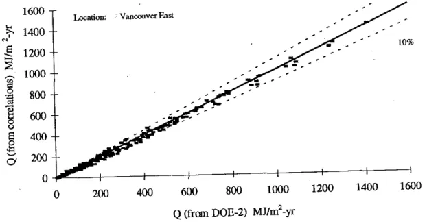
of the DOE-2.1E simulations. Figure 3 shows how the annual heating system loads; Q, for Vancouver calcu-lated using the climate correlations agree with the sys-tem loads obtained using DOE-21E. When using the (19)

600

800

1000

1200

Q (fromDOE-2) MJ/m2-yr

400

200

Location: VancouverEast

Location: OttawaEast

1600

....

1400

>. N

,

ｾ

1200

1000 ｾ

rg

.g

₈₀₀

os

ｾ

600

u

S

400

0 ｾ ｾ

200

0

0

0

2000 1800 1600 ｾ 1400 ｾ

ｾ

1200 ::E R 1000

'"

8 800 § S ₆₀₀ CI 400 200 0 0

Figure3 Comparison of annual heating system loads. Q calculated using climate correlations with loads predicted by DOE-2. 7E for l{ancouver.

500 1000 1500

Q",""""d) =L' SGRF' IGRF' GIF MJ/m 2

-xr

Figure2 Comparison of annuai heating system ioads. Q caicuiated using heating equations with ioads predicted by DOE-2. lEfor Ottawa.

EnvelopesVI/Building Energy Codes-Principies

= So+Sl .CDD50+S2 .VS_ew+S3 .LAT ｾ = k2 .ｾ ｬｯ ｴｴ ｡ ｷ 3 ｾ = k2 .ｾ ＳＰ ｴｴ ｡ ｷ 2 ｾ = k2 •ｾ Ｒ ｯ ｴｴ ｡ ｷ

the value of

kz

isfirst calculated from Equation 19. RFisthen calculated using Equation4and the follow-g coefficients:

1400 10% 1000 1200 800 1000 800 600

A methodology was developed for predicting the effect of envelope thermal characteristics onenergy use in commercial buildings. Part of the methodology con· sists of methods for conducting a parametric study of the perimeter zones of a model building for the climates of interest (Crawley 1992). The result of the parametric studies can be used to generate coefficients for simplified models predicting energy use. If several parametric stud-ies are done, then climate correlations can be developed

SUMMARY

600 400 400 VancouverEast 200 Locatioo: 1000 900 800 700 600 500 400 300 200 100

O ¥ ' - - - + - - - - I - - - + - - - + - - - - I

o

1400 1200

!f.

N 1000

a

ｾ ｾ

::E

ｾ 800 ｾ ｾ 0 ₆₀₀ 0

a

0 ₄₀₀ <l:: ｾ U 200 ｾ 0 0 200

Thermal EnvelopesVII Building Energy Codes-Principles

Figure5 Comparison of annual cooflng system loads,C, calculated using climate correiatlons with ioads predicted by DOE-2.7E for Vancouver East orientation.

'"

C (predicted) MJ/m2-yr

C (from DOE-2) MJ/m2_yr

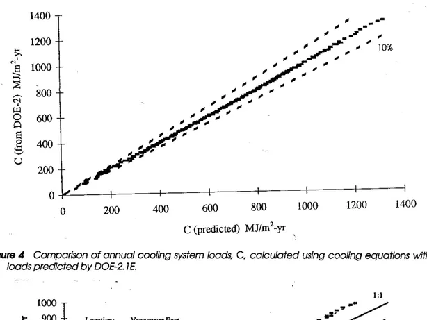
Figure4 Comparison of annuai cooiing system ioads, C, caiculated using cooling equations with ioads predicted by DOE-2.7E.

1:1

climate correlations, the results are within 10% for typi-cal heating loads. Figure 4 shows how the predicted val-ues, C, compare with the DOE-2.1£-generated cooling loads. The predictions are within 10% of the simulated values. It was possible to generate climate correlations for the coefficients for the cooling equations. For most regions in Canada, cooling loads can be calculated within 10% of the DOE-2.1£ results. Figure5shows the agreement between the cooling loads calculated using the climate correlations for Vancouver and the DOE-2.1E simulations.

to extend the models to locations not simulated. The models consist of straightforward methods for calculat-ing the heatcalculat-ing and coolcalculat-ing system loads. The system loads are calculated using the three decoupled envelope parameters, U (thermal transmittance), V (solar gain), andW (internal gains). The heating system loads are cal-culated by progressively modifying the annual heat loss to account for solar gain, internal gain, and solar and internal gain interaction. The annual heat loss was shown to be a linear function of U, the slope and inter-cept being dependent on climate. The slope and interinter-cept also were shown to vary linearly with heating degree-days. Climate correlations were developed for the solar gain reduction factor,SGRF, by shifting the curves of the location in question to a specific location. A similar method was developed to account for internal gains; however, the internal gain reduction factor, IGRF, was found to be independent of orientation. A similar method was derived for cooling.It was found that cool-ing loads could be calculated as the sum of a base coolcool-ing load and a correction term for transmission. The base cooling was found to vary linearly with the solar gain and internal gain parameters. A minimum cooling load, a result of the HVAC system modeled and the minimum ventilation requirement, also was found to occur. The models are robust and predict energy use well in moder-ate to extreme Canadian climmoder-ates, unlike other correla-tion models that were generated for predominantly cool climates. The methodology has been extended to include hot climates and it appears to be independent of climate, HVAC system, and operational assumptions (Thomas and Prasad 1995).

REFERENCES

ASHRAE. 1989.ANSI/ASHRAE Standard 62-1989, Ventilation for acceptable indoor air quality.Atlanta: American Society of

Thermal Envelopes VIIBuilding Energy Codes-Principles

ｾｾｾｾ ＭＭＭＭＭ ｟ Ｎ ｟ ＭＭＭＭＭ

Heating, Refrigerating and Air-Conditioning Engineers, Inc.

Cornick S.M., and D.M. Sander. 1994. Development of heating and cooling equations to predict changes in energy use due to changes in building thermal envelope characteris-tics. Internal Report IRC-IR-656. Ottawa, ON: Institute for

ResearchinConstruction.

Cornick, S.M., and D.M. Sander. 1995. The effect of mass on the prescriptive levels in the energy code for buildings. Com-mittee Paper. 31st Meeting of Standing ComCom-mittee on Energy Conservation in Buildings. Ottawa, ON: Institute for Research in Construction.

Crawley, D.B. 1992. Development of procedures for determin-ing thermal envelope requirements for code for energy efficiency in new buildings (except houses). Ottawa, ON: Institute for Research in Construction, and Marlin, TN: D.B. Crawley Consulting.

NRCe. 1994.Thenational energy code

for

buildings(1995). Public Review Draft 1.0. Ottawa, ON: National Research Council ofCanada.

Sander, D.M., and S.A. Barakat. 1983. A method for estimating the utilization of solar gains through windows.ASHRAE Transactions89(1): 12-22.

Sander, D.M., and S.A. Barakat. 1984. Mass and glass: How much, how little?ASHRAE Journal26(4): 26-30.

Sander, D.M., and S.M. Cornick. 1994. Calculation metlwd for envelope tradeoff compliance for the national energy code.IRC Internal Report IRC-IR-657. Ottawa, ON: Institute for

ResearchinConstruction.

Sander, D.M., S. Cornick, G.R. Newsham, and D.B. Crawley. 1993. Development of a simple model to relate heating and cooling energy to envelope thermal characteristics. Presented at3rd International Conference on Building Simu-lation.Adelaide, Australia: International Building

Perfor-mance Simulation Association.

Sander, D.M., M.e. Swinton, S.M. Cornick, and J.e. Haysom. 1995. Determination of building envelope requirements for the (Canadian) national energy code for buildings. To appear inThermal Performance of the Exterior Envelopes of Buildings VI,Clearwater, FL.

Thomas, r.e., and D.K. Prasad. 1995. Energy efficient building envelopes-An Australian perspective. To appear in Ther-mal Performance of the Exterior Envelopes

of

Buildings VI, Clearwater, FL.