Applications of Finite Difference Synthetic Acoustic Logs

135

APPIJCATIONS OF FINITE DIFFERENCE

SYNTHETIC ACOUSTIC LOGS

by

R.A. Stephen· and F. Pardo-Casas Earth Resources Laboratory

Department ofEarth. Atmospheric and Planetary Sciences Massachusetts Institute of Technology

Cambridge,lIA 02139

ABSTRACT

Finite difference synthetic acoustic logs are suitable for studying wave propagation in vertically varying boreholes and in boreholes with continuously varying properties. Snapshots for the traditional smooth bore in a homogeneous rock show the standard phases in the borehole (compressional and shear head waves, pseudo-Rayleigh waves, and Stoneley waves), and also display the complex wave interaction which occurs in the rock. If a simple gradient in elastic parameters and density replaces the sharp interface the shear head wave and pseudo-Rayleigh wave are strongly attenuated. Also, off-centered receivers, washouts and horizontal fissures can have significant effects on amplitudes. A thorough understanding of these effects by forward modelling is essential in order to avoid pitfalls in interpretation and in order to design robust schemes for obtaining elastic properties and attenuation from acoustic logs.

INTRODUCTION

The finite difference method for synthetic acoustic logs was presented in Stephen et al. (1983) and the stability and accuracy of the technique was demonstrated. This paper discusses applications of the method by considering some canonical examples.

The first set of examples consists of vertically homogeneous models with step, gradient, and step-gradient velocity-radius functions. The effects of smooth rather than sharp velocity contrasts are demonstrated. An example of the effect of an off-centered receiver is included and the amplitude of multiples is discussed.

The second set of examples demonstrates the effect of a washout at different positions relative to the tool. The washout model is an example of a medium which varies in two dimensions.

136 _{Stephen and Pardo-Casas}

The third set of examples demonstrates the effect of horizontal fractures intersecting the well bore at the tool.

MODEL PARAllETERS

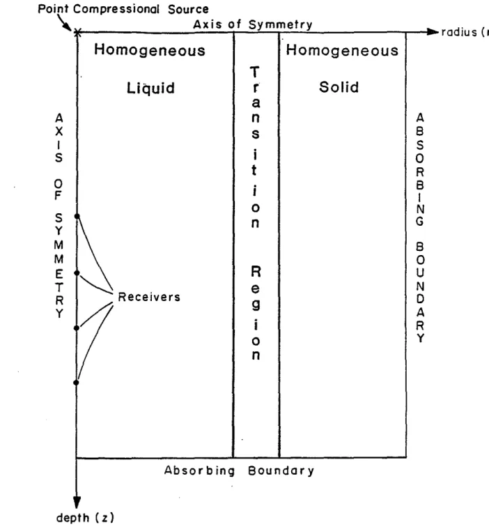
Figure 1 shows the geometry used for the calculations. Ail models considered in this paper are 0.6 m wide by 3.0 m long (60 grid points by 300 grid points at 0.01 m per grid point) and time series are generated out to 2.5 msecs (1250 time steps at 0.002 msec per step). Unless otherwise noted, a compressional point source is located at the center of a 0.1 m radius borehole and receivers are placed at the center of the borehole at increments of 0.2 m between 1.6 and 2.8 m below the source. (Pardo-Casas et at., this volume, discuss the effects of a rigid tool in the borehole.) The source waveforms and spectra are shown in Figure 2. The center frequency in pressure is 15kHz and the upper half power frequency is 20kHz.

VERTICAUX HOMOGENEOUS MODELS

The first example is a sharp interface between a fiuld-filled borehole and a homogeneous formation. This model represents a clean, mud-filled bore in a rock with velocities similar to those of a well consolidated sandstone. Figure 3 shows (a) the velocity and density functions, (b) the time series plots and (c) the snapshots for this model. The compressional and shear head waves and the Stoneley and pseudo-Rayleigh waves can be identified on the time series plots. This example was used for a comparison between finite difference and discrete wavenumber methods by Stephen et al. (1983) and good agreement was obtained.

The snapshots show how the various phases evolve as they propagate down the well bore. The transmitted compressional wave can be readily identified as the lowermost disturbance in the rock which reaches the bottom of the grid at 0.8 msec. This wavefront intersects the borehole at right angles. To the left of this arrival, in the well bore, is the conical wave or compressional head wave. Note also a wavefront at approximately thirty degrees from the interface, which intersects the interface at the same point as the compressional transmitted and head waves (at time steps 0.4, 0.6 and 0.8 msec). This is a shear wave converted at the forward edge of the transmitted wave at the same time as the compressional head wave. (It is described by Brekhovskikh, 1960, as P1P2S2). If this wave front is followed back into the solid one sees that it is tangential to a higher amplitude short wavelength arrival which is the "transmitted" shear wave. This shear wave was converted at the borehole wall from the incident compressional wave. Between the transmitted compressional and shear arrivals one can also see the progressive deveiopment of compressional wave multiples or "leaking" PL modes. The lowermost large amplitude arrival in the well bore, which is coincident with the "transmitted" shear wave in the rock, is the onset of the pseudo-Rayleigh wave packet. This packet becomes broader with time demonstrating its dispersive nature. Towards the middle of the packet (for example at 1.2 msec) the wavelength shortens indicating the Stoneley wave. Note that the velocity of this arrival is lower than the velocity of the onset of the pseudo-Rayleigh wave. Above the Stoneley wave is the still shorter wavelength Airy phase of the pseudo-Rayleigh wave. The amplitude of the high

(

FIniteDitIerence Applications 137

energy packet dies away qUickiy in the rock leaving a complex pattern of body waves which are the remanents of compressional and shear wave multiples (leaking PL and SL modes).

The effect of an off-centered receiver for the sharp interface model is shown in Figure 4. Receiver distance from the center of the borehole is increased in increments of 0.02 m from 0.0 to 0.08 m. The amplitudes of all phases decrease rapidly with increasing radius (approximately 12 db across the borehole). Also the relative amplitudes of the multiples become more uniform and the multiples themselves become less distinct. This example can be compared with Willis et

at.

as a discriminant for particular phenomena correct centering of the tool is essentiaL

The second example (Figure 5) is a linear velocity gradient between the ftuid-filled well and the formation. This model represents a borehole in an altered formation. The shear wave coupling is reduced by the gradient and the shear head waves and pseudo-Rayleigh waves are not observed. The compressional and Stoneley wave amplitUdes are greater than for the sharp interface case (Figure 3) because less energy is lost to shear. The P head wave velocity (3.9 lcm! s, Figure 5b) corresponds closely to the formation velocity (4.0 lcm! s). However the Stoneley wave arrivaL which could be mistaken for a

shear or pseudo-Rayleigh wave arrival if attention was not paid to waveform, is travelling at the borehole mud velocity (1.8lcm! s). Care should be taken when

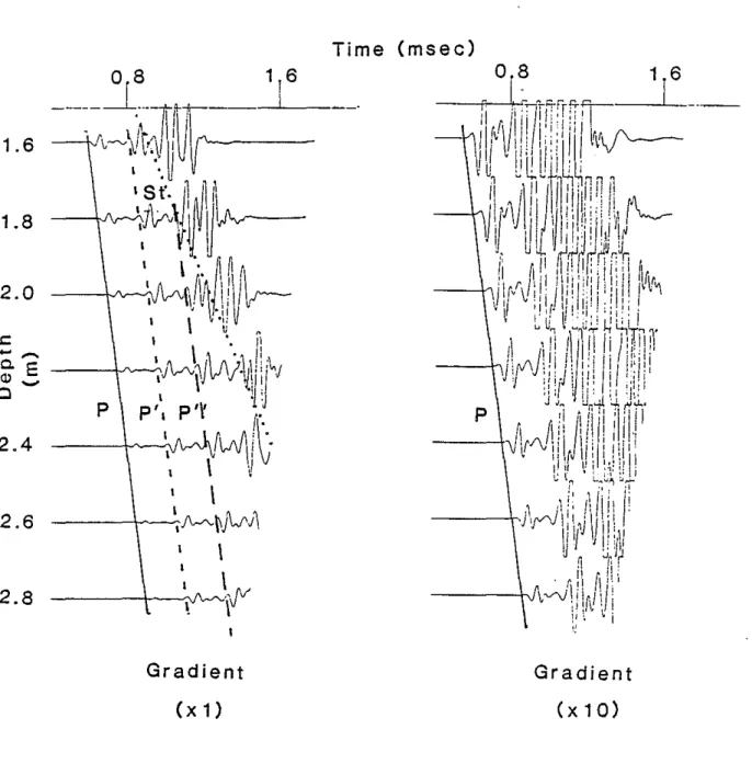
interpreting logs obtained in formations where this model may apply. Good estimates of the formation shear wave velocity may be impossible to obtain ·from full waveform data. Also note the progressively higher amplitudes of the compressional wave multiples. An event detecting deVice set to pick the Stone ley wave arrival on an amplitude basis could easily pick the third multiple, P". The higher amplitude multiples will be discussed further below.

The snapshots for the gradient model (Figure 5c) are simpler than for the sharp interface case because of the absence of shear waves and pseudo-Rayleigh waves. The transmitted compressional wave, compressional head wave and compressional wave multiples (leaky PL modes) can readily be identified. The nature of the Stoneley wave without the interference of the pseudo-Rayleigh wave can also be observed. This wave shows considerably less dispersion than the pseudo-Rayleigh wave in Figure 3c.

Similar phenomena are observed in the sharp-interface /linear-gradient combination (Figure 6). This model is more realistic than the simple gradient model because it includes a discontinuity in properties at the borehole wall.

The P head wave velocity (Figure 6b) corresponds to the formation (3.9lcm! s).

The next large amplitude pick lacks coherence but has a velocity of 1.8 lcm! s .

This corresponds to a shear or pseudo-Rayleigh wave travelling at the near hole (or damaged zone) shear wave velocity (1.6-1.8 lcm! s). Poisson's ratio estimates based on logs where this sort of model is valid will be biased towards higher values. The pseudo-Rayleigh wave is about twice as large (6 db) for this model as for the sharp interface model(Figure 3). Coupling to shear wave effects is improved because the effective shear wave velocity in the solid is closer to the compressional wave velocity in the fiuid (compare Figures 6a and 3a).

138

Stephen and Pardo-Casas

Compressional wave multiples are evident in the gradient model '(Figure 5b). The amplitude of the first P head wave decreases rapidly with depth and the second and third P arrivals are progressively higher in amplitude. Why, for example, is the second P arrival (the first mUltiple) larger than the first P arrival (the P head wave)? One answer is that the P head wave spends more of its time as a head wave than a body wave. For a Cartesian geometry head waves decay much more rapidly with range (as 1/r2) than body waves (as

..J 1/ r.dp / dr). (For example the compressional head wave in Figure 5 decays

to about a quarter (-12 db) between 1.6 and 2.8 m depth because the arrival at the deeper receiver has travelled twice as far as a head wave.) To see this more clearly consider the ray diagram (Figure 7) which corresponds to the velocity-radius profile of the gradient model. The P head wave and the first multiple ray paths are shown. The solid ray paths correspond to body waves and the dashed ray paths to head waves. The paths are the same for the head wave and first multiple except in the region marked "A." In this region the first multiple travels 10.2 units as a body wave over the same vertical distance that 'the primary wave travels as a head wave (7.5 units). Using the Cartesian assumption, the head: wave has decayed by (1/7.5)2 or 1/56 over this distance. The corresponding decay for the first multiple in this section is only

..J1/r.dp/dr or 1/14.3. (It is assumed here that the first multiple does not lose

energy at its turning point. This is consistent with WKBJ theory, e.g. Chapman, 1978, where turning rays are only subject to a phase shift of ninety degrees.) Thus the primary path is attenuated four times as much as the first multiple path. This ratio is confirmed by inspection of Figure 5. The amplitude of the first multiple at 2.8 m depth is very similar to the amplitude of the primary at 1.6 m depth.

WASHour MODElS

The next series of models investigates the effects of washouts in the borehole wall on acoustic logs (Figure 8). The continuous gradient model (Figure 4) is perturbed by introducing a depth: dependent borehole radius. The washout is placed at four locations relative to the source of the tool: directly opposite the source at depth 0.0 m, at 0.8 m, at 1.6 m, and at 2.4 m below the source. Strangely enough the washout directly opposite the source has little effect on the compressional wave signals (Figure 8a). The primary compressional wave is twice as large (6 db) as when the washout was not present but the first and second multiples are considerably less affected. Presumably the steeper ray paths which contribute to the multiples are less affected by the washout. The Stoneley wave on the other hand is dramatically affected, being less in amplitude by about 3 or 4 db and at the 1.6 m receiver is about half the pulse-width. Energy seems to be lost by reverberation in the cavity, which is evident on the snapshots (Figure 8b).

The washout at 0.8 m below the source (Figure 8c) has essentially no effect on the primary compressional wave but the uppermost 0.4 m of the multiples P' and P" are larger by 3-4 db than without the washout. The washout has an apparent tendency to focus the compressional wave energy to certain depths. As with the 0.0 m washout the Stone ley wave is much lower in amplitude (approximately -6db) and is less dispersed. The Stoneley waves tend to oscillate being first smaller (at 1.6 m), then larger (at 1.8 m), then smaller (at 2.0 m),then larger (at 2.2 m), then smaller again (at 2.4 m). The presence of

(

(

Finite Difference Applications ₁₃₉

the washout apparently causes a "beating" of these phases as they propagate down the well bore. Stoneley wave retlections from the washout can be seen in the snapshots (Figure 8d).

The washout at 1.6 m (Figure 8e) is directly opposite the top receiver. Note that the trace at the top receiver for this model is identical to the top receiver trace for the washout at 0.0 m. This is a demonstration of source-receiver reciprocity. I=ediateiy below the washout (at 1.8 m) the compressional wave phases are higher in amplitude by 3-9 db. Below this the primary compressional wave returns to normal. the tlrst P-wave multiple is anomalously low (at 2.2m), and the secondP wave multiple and Stoneley wave are dramatically higher. Beating in these latter phases is not evident.

The final washout model (Figure 8g) has the washout at 2.4 m depth, opposite the middle of the array. Again the tlrst and second P arrivals are higher in amplitude just below the washout (2.6 m) but decay quickly below that. There Is no evidence of retlections of these phases back up the borehole.

These examples demonstrate some of the effects which washouts can cause on full waveform logs. Amplitudes of compressional waves can increase and decrease by up to 6 db depending on the location of the receiver relative to the washout. Washouts tend to decrease the dispersion and amplitude of the Stoneley waves but beating effects are apparently stimulated. The compressional body waves tend to follow the washout deformation and, except for some focussing. are little affected. The Stoneley waves, on the other hand. retlect from the change in thickness of the waveguide.

HORIZONTAL FISSURES

The effect of horizontal fissures on full waveform logs was studied using two models: a 10.0 em thick tlssure was placed at 0.8 and 2.2 m below the source. Gradients similar to those used in Figure 5 were introduced above and below the tlssure for its full length.

The effects of the fissure at 0.8 m are essentially indistinguishable from the washout at the same depth (cf. Figure 9a with Figure 8c). The first P wave amplitude is the same as the unmodified borehole amplitude. The second P wave arrival has very large amplitude at the 1.6 m receiver but decays qUickly with depth. The same beating phenomena is present in the Stoneley wave arrival that was mentioned above. Stoneley waves refiect from the fissure but remarkably little energy is actually trapped in the fissure.

When the fissure is placed opposite the middle of the receiver section the effect of transmissions and retlections on the compressional waves can be observed (Figure 9c). Directly opposite the fissure (at 2.2 m) the P wave arrivals are in a shadow zone, but below the fissure the amplitude is unchanged.

140

Stephen and Pardo-Casas

CONCLUSIONS

Synthetic full wave form acoustic logs are a useful instructive tool for studying wave propagation in boreholes. The snapshot formats show clearly the evolution and conversion of the various phases. Even for depth independent media the snapshots provide interesting insights into the propagation.

The finite difference technique is well suited to depth dependent problems and some examples were presented above. Body waves seem to be little affected by washouts and horizontal fissures. Refiections and "beating" phenomena associated with the waShouts and fissures has been demonstrated for the Stone ley waves.

Frequency-wavenumber analysis in a similar fashion to Kelly (1983) would give further insight into the effects on the guided wave phenomena. Dispersion relations for vertically inhomogeneous models couid be compared with the analytical results of Biot (1952) for vertically homogeneous models. Future work should also include attenuation and applications to real data. The true value of synthetic acoustic logs cannot be assessed until some comparison with real data is made.

ACKNOWLEDGEMENT

This research was supported by the Full Waveform Acoustic Logging Consortium at M.LT.

REFERENCES

Biot, M.A., 1952, Propagation of elastic waves in a cylindrical bore containing a fiuid: J. appl. Phys., 23, 997-1005.

Brekhovskikh, L.M., 1960, Waves in layered media. Academic Press, New York. Chapman, C.H. 1978, A new method for computing synthetic seismograms:

Geophys. J.R Astr. Soc., 54,481-518.

Kelly, K.R, 1983, Numerical study of Love wave propagation: Geophysics, 48, 833-853.

Stephen, RA., Pardo-Casas, F., Cheng, C.H., 1983, Finite difference synthetic acoustic logs: M.LT. Full Waveform Acoustic Logging Consortium Annual Report, Paper 4.

Willis, M.E., Toksoz, M.N., and Cheng,C.H., 1983, Approximate et!ects of otl'-center acoustic sondes and elliptic boreholes on full waveform logs: M.LT. Full Waveform Acoustic Logging Consortium Annual Report, Paper 5.

(

(

(

(

FIniteDifference Applications 141 radius (r) Source Axis of Symmetry

-Homogeneous

Homogeneous

T

Liquid

r

Solid

a

n

s

i

₀

S

t

R

i

n

G

0

~R

R

u

e

r1 """"

9

0

i

R

n

X

S

o

S

T

"

Figure 1: Outline of the geometry used for finite difference synthetic acoustic logs. A compressional point source is located at the intersection of verti-cal and horizontal axes of symmetry. A vertical transition region separates the fiuid in the well bore from the solid rock. The transition re-gion has arbitrary thickness and can represent sharp vertical interfaces or continuous two dimensional variations of compressional and shear wave velocity and density.

142 _{Stephen and Pardo-Casas}

(

Waveforms

Potential at Origin

Far Field Displacement

Pressure

Ampli tude Spectra

( ( ( (

..

0.2 msec

..

o

Frequency (kHz)

45

Figure 2: Source waveforms and amplitude spectra for the examples shown in this paper. The peak frequency in pressure is 15kHz and the upper half-power frequency is 20kHz. The pressure pulse duration is 0.2msec.

FiniteDi1rerence Applications 143 /

DEPTH

(M)

0.2

0.4

0.6

I

I

I

I

0.0

o

w

en

... 2.0 -

S

::E

...

>-

r-g

>

p

0.0

0.2

0.4

0.6

0

I

I

I

1.0

...

i'-::E

...

>-

r-en

2.0

Figure 3a: The velocity and density profiles, typical of a mud filled hole in sand-stone, are shown. This is a sharp interface model for a vertically homo-geneous case.

144 ( Stephen and Pardo-Casas

( ( ( !

Time

_~J\

_{.\ \/}

'.~ i\j~N-r

~~~

,V

.

'.~v\jW

p

_S

\

_\

s'

_t·

_I

'~'vv~!v

_,

_.

.

.

2.6

2.0

1.6

-

...

E

o

2.8

2.4

Sharp Interface

Sharp Interface

Figure 3b: The time series format for the sharp interface modei shows the tradi-tional waves expected for a point source in a borehole. The compressional p, shear S,and Stoneley St arrivals are indicated. The velocities are 4.0,

2.1,1.8 km/s respectively. The receivers are located on the axis of

Finite Difference Applications ₁₄₅

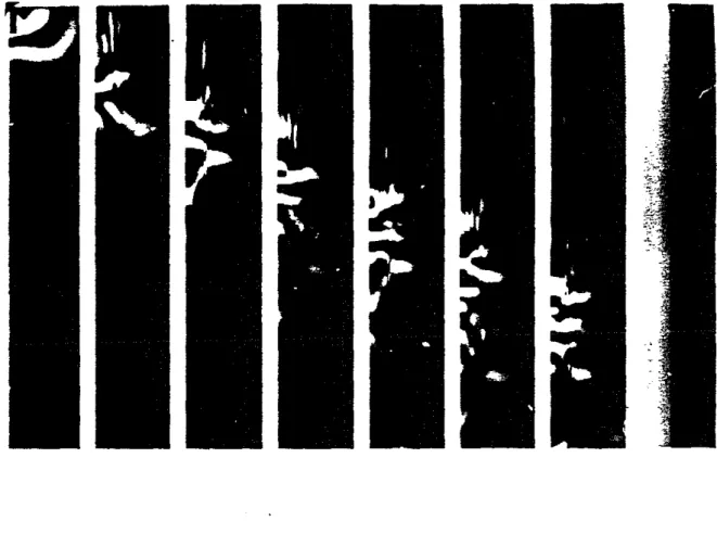
Figure 3c: The complete picture of wave interaction around the borehole for the sharp interface model is shown in the snapshot format. A description of this figure is given in the text. The first six frames show the amplitude distribution of the the vertical displacement field in radius-depth space. Each frame is 0.6 m wide by 3,0 m deep. Time progresses from 0,2 msec to 1.4 msec. The eighth frame is a representation of the velocity field.

146 _{Stephen and Pardo-Casas} RECEIVER RADIUS (0m) (

~

j

".

~

Ilil:

- - - j iJ\!I-,J\"'~ ,.,ili·' i" i"I:I":;:J''vvv'V\pO O~JV\r'\j"""I~ , J IfI " 1

I'

Ii

:,iI ,:' ,)"

_sf

,..

\J\

i\

i:

Ii

~:\

----yv-vv'VV"v""V 1\ i, ,1"J\:'.~I:t:~-6 0 .L....-A_.../\..)t

'\11""-I

J

' '

:J

\J

l

(x 1 0) _{SI:iARP INTERFACE (2.2 M DEPTH) (x 1)}

Figure 4: The variation of response across the borehoie is shown here at two gains (xl. xlO) for the sharp interface model. The amplitude of all phases decreases rapidly with increasing radius, Note that the Airy phase is essentially non existent at the 8.0 em location,

FiniteDi1I'erence ApplicatioIlB 147

0.0

°

-

u

w

2.01--...

>-....

g

4.0

>

DEPTH (M)

0.2

0.4

'\

S

,---p

0.6

0°....

·°_-,-_ _

°,...·2_-,-_ _

0,....4_-,-_0...,.6

>-....

en

z

2.0

w

u

u

:E

1.0

1 - -...

Figure 5a: The veiocity density functions are given for a simple gradient model which represents a severely altered borehole.

148 1.6 1.8

2.0

2.4

2.6

2.8

Stephen and Pardo-Casas

Time (msec)

Gradient

(x 10)

(

Figure 5b: The time series plots for the gradient model show the compressional head wave P, the compressional wave multiples p', p", and the Stoneley

wave St. The compressional waves have a velocity of 3.9 kmls and the Stoneley wave has a velocity of 1.45kmls.

Finite Difference Applications 149

Figure 50: The snapshots for the simple gradient model are shown. The dimen-sions are the same as for Figure 30.

150 Stephen and Pardo-Casas

0.6

(M)

0.4

DEPTH

0.2

0.0

O.----,..--,..--.,..--"T"""--.---,

p

u

4.0

o

>

~

1--.., ...

"

2.0

...

S

0.0

0.2

0.4

0.6

I

I

I

--

u

u

1.0

-"

--

2.0

Figure Sa: The velocity and density functions for the combination of a sharp in-terface With a gradient zone behind it. This model is more representative of an altered borehole than the simple gradient model (Figure 5).

FiniteDi1ference Applications ₁₅₁ Time (msec) ,

,"

0.8

1 6

____- L

_

I/\f~~~---,

-~VV'-\v.7J\N\:JIrv~

---+~\~\j~J\j\J~

S

---t~~,Jh'.<v/I/VV!r\!\r'~

_~

--+----./'-Ar--J\"-J'v

V'v\JV~WN

1.6

1.8

2.0

-

...

_E

e

_p

2.4

2.6

2.8

Sharp Interface / Gradient

(x 1)

Sharp Interface / Gradient

(x 10)

Figure Sb: The time series lormat lor the sharp interlace/ gradient modeL The velocities 01 the compressional P and shear S arrivals in the time series plot are 3.9 and 1.8 kml s respectively. The P wave is sensitive to the lor-mation but the shear wave is "Ieeling" the altered zone.

J:P2

(

FInite Di1Ierence Applications

153

1:-

I:

-T

Figure 7: For the simpie gradient model, multiples are larger in amplitude than the primary because they travel more of their path as body waves and less as head waves. In the section marked "A" where the primary and first multiple differ. the first multiple loses less energy as a body wave (solid line) even though it travels farther than the primary which travels as a head wave (dashed line).

StephenandPardo-Casas Time (msec) 1.6

1.8

"

--~~ji)V\j:::i1y

o

8

1.6

--~'-r-~----,fM~~V/~

-J\J"\IW\i\~\r--1

f'

2.0

--Jv--\A.,vV~~~A--j~

2.4

--Jv'4!VvI/~vJ

2.6

(x

Gradient Without Washout

(x 1)

Figure 8a: A comparison of time series and snapshots for gradient modeis with washouts at four depths relative to the tool is shown in this sequence of figures, The effects are discussed in the text. This figure is the time series format for the washout at 0.0 m.

Finite Difference Applications 155

156 Stephen and Pardo-Casas Time (msec) ( f, "

2.4

~WV\rJVI

1.6

2.0

-

_Q.E

_ _

0

8 ,

~-_.

~\fV\!JIJ~--

_,

~jVV\J

Jij'v--~A.Aj'VVVJ~

~J~J~V\j~\JV~

Gradient Without Washout

(

Yinite DI1Ierence Applications 157

158 Stephen and Pardo-Casas ( ( ( (

1 6

_--l[

_

__°-lL

1__

~

_ _

11_6__

--JvvV~~'\--JV_vV\t;~~~

2.0~~~\ll~

i~~~~I~

I

I-t' :\

2.4

~VV"\V\

2.8

Washout at 1.6m _{Gradient Without Washout}

(x 1) _{(x 1)}

FiniteDitrerence Applications 159

160 Stephen and Pardo-Casas

1.6

2.0

0.8

1.6

___I " .

I

~~~\~~V~'----1.8

-VV4Vv\j11~1ik­

~~VJWlr-

_,

Ii

~J~IIJVV\\liJ

2.4

-....

E

o

J1t--'\j\rvij\

Washout at 2.4m Gradient Without Washout

(x1) (x 1)

Finite Ditlerence Applications 161

162 Stephen andPardo-Casas Time (msec)

2.0

~~"\fvVIr~

1

~ ~JY,J~tlJ\V\jl

~[

t

f\rv!\r~-\ II

\

~J\~~\r~

---~J\-NIJ\,;VV\i\!v

,

jwv)

Gradient Without Fissure

(x 1)

Figure 9a: This sequence of figures shows a comparison of time series and snapshots for gradient models with horizontal fissures at two depths rela-tive to the tool. The effects are discussed in the text. This figure is the time series format for the fissure at 0.8 m_

Finite Difference Applications

Figure 9b: Snapshots for the fissure at 0.8 m.

164 StephenandPardo-Casas Time (msec) ( (

1.6

2.0

_...

E

o

2.4

2.6

Gradient Without Fissure (x 1 )

Yinite Di1Ierence Applications 165.

166 ( ( ( ( ( (