HAL Id: hal-02908146
https://hal.archives-ouvertes.fr/hal-02908146
Submitted on 23 Sep 2020HAL is a multi-disciplinary open access
archive for the deposit and dissemination of sci-entific research documents, whether they are pub-lished or not. The documents may come from teaching and research institutions in France or abroad, or from public or private research centers.
L’archive ouverte pluridisciplinaire HAL, est destinée au dépôt et à la diffusion de documents scientifiques de niveau recherche, publiés ou non, émanant des établissements d’enseignement et de recherche français ou étrangers, des laboratoires publics ou privés.
The effect of sharp-edge acoustic streaming on mixing in
a microchannel
Chuanyu Zhang, Xiaofeng Guo, Philippe Brunet, Laurent Royon
To cite this version:
Chuanyu Zhang, Xiaofeng Guo, Philippe Brunet, Laurent Royon. The effect of sharp-edge acoustic streaming on mixing in a microchannel. Annales de congrès SFT 2020, 2020, �10.25855/SFT2020-041�. �hal-02908146�
The effect of sharp-edge acoustic streaming on
mixing in a microchannel
Chuanyu ZHANG1, Xiaofeng GUO1,2∗,Philippe BRUNET3, Laurent ROYON1
1Universit´e de Paris, LIED, UMR 8236, CNRS, F-75013, Paris, France. 2Universit´e Gustave Eiffel, ESIEE Paris, F-93162, Noisy le Grand, France. 3Universit´e de Paris, MSC, UMR 7057, CNRS, F-75013, Paris, France. ∗Corresponding author: [email protected]
Abstract - Strong Acoustic Streaming (AS) in a liquid can be generated near sharp-edge structures inside a microchannel. In this study, an experimental setup containing a Y-mixer and a sharp-edge patterned microchannel excited by a piezo-transducer is built. Based on visualisation and Iodide-Iodate Reactions, both macro- and micro-mixing performance are investigated. Results show that acoustic streaming allows a decrease of micromixing time from 0.3 s to 0.04 s. Meanwhile, the mixing enhancement by AS is very sensitive to the channel throughput, as the residence time becomes shorter at higher flowrates. Keywords: Acoustic Streaming; Micromixer; Process Intensification; Macro-mixing; Micro-mixing. Nomenclature
Vi input voltage to piezoelectric transducer
vs streaming velocity
vω acoustic vibration velocity
f frequency rc curvature radius Qc channel throughput w width of channel XS Segregation Index tm Micromixing time Greek symbols
α tip angle of the sharp edge
αv volumetric flow rate ratio between two inlets
δ acoustic boundary layer
1. Introduction
Acoustic streaming (AS), which is the steady time-averaged flow generated by acoustic fields, was first observed more than a century ago. From the perspective of energy conver-sion, the streaming phenomenon originates from the dissipation of the acoustic energy due to the viscosity of the fluid. Recently, strong streaming flow around sharp structures actuated by kHz level acoustic vibration has been observed [1, 2, 3]. Thanks to its non-invasive nature, powerful disturbances within a laminar flow together with low-cost equipment requirement, such a sound-driven steady flow has promising potential applications in Process Intensification (PI), for example the mixing of two or several fluids in continuous mode, or heat convection enhancement.
The principal advantage of low-frequency sharp-edge AS is its low power input, avoiding local heating effect from piezoelectric actuators. Comparatively, common acoustic streaming is less efficient, for example those generated in Kundt’s tubes using kHz-range acoustic forcing [4], or in microfluidic channels using transducers in pairs or with reflectors in order to real-ize a condition of resonance. In the latter situation, the acoustic wavelength has to be of the same order as the channel width, which imposes a frequency in the MHz range. Conversely, strong streaming around a sharp edge can be easily induced by low-cost piezo-transducers with frequencies of a few kHz or lower. Contrary to MHz-range transducers, in this situation the
wavelength of the audible acoustic wave at several kHz (λ ≈ 0.5 m) is much larger than the characteristic dimensions of microfluidic devices (typically lower than 1 mm), which means the acoustic vibration within the fluid is homogeneous in amplitude and has the same phase every-where. Moreover, the phenomena of acoustic and fluid mechanics are highly coupled, making studies of sharp-edge AS challenging.
2. Theoretical background
2.1. Origin of Acoustic Streaming around sharp edge
The sharp-edge AS in this study uses acoustic wavelength λc = c/f , of the order of one
or a few meters, hence much larger than the characteristic flow dimensions, as the height of the sharp edge or width of the channel is typically smaller than 1 mm). Both acoustic and streaming velocities being much lower than the sound speed (c=1430 m/s in water), the flow in the present study can thus be treated as incompressible. In the classical analytical treatment of streaming, the time-averaged Navier-Stokes and the mass conservation equations in Eq.1 and Eq.2 [1], include a first-order, time-dependent acoustic velocity vω and a second-order mean
flow (streaming velocity) vs:
(vs· ∇)vs= − 1 ρ∇ps− Fs+ ν∇ 2 vs (1) ∇ · vs= 0 (2)
Here, Fs = 12Re[(vω · ∇)vωT] is the time averaged inertia term due to the first-order acoustic
field, and is treated as a steady force term that can induce the second-order steady streaming flow.
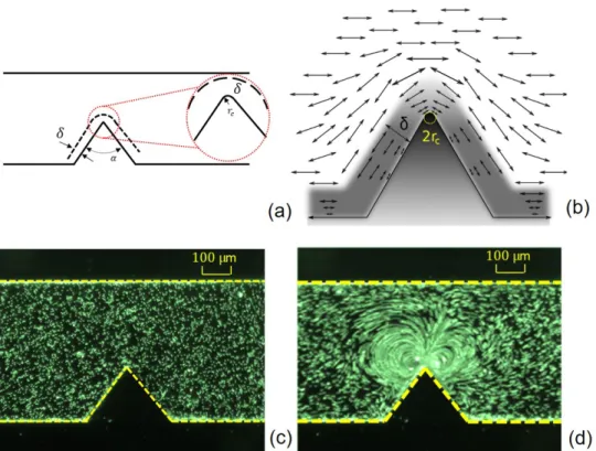
From the form of Fs, it is clear that a homogeneous acoustic field cannot generate any
stream-ing flow, as the effective force would be null. However, the sharp tip structures (Fig.1 (a)) with strong local curvature on the channel walls induce strong heterogeneity in the acoustic oscil-lating flow in the fluid. As sketched in Fig.1 (b), at a given time, the vibration of the fluid is uniformly distributed except for the local zone close to the sharp edge. More specifically, close to the tip, both the orientation of the acoustic field and the vibration amplitude provide favorable conditions to induce an intense Fsvery near the tip, via a centrifugal acceleration[2]. Far from
the tip, the force is null or negligible. Therefore, the sharp edge induced non-uniformity of the acoustic field makes acoustic streaming at relatively low frequency (several kHz) possible (see Fig.1 (c) with acoustic OFF and Fig.1 (d) acoustic ON).
2.2. Iodide-Iodate reaction and Segregation Index
Competitive Iodide-Iodate reaction, also named the Villermaux-Dushman method [5, 6], is employed to evaluate the micromixing performance of the microchannel with acoustic stream-ing. This reaction scheme is sensitive to mixing at the molecular scale and the detection of iodine (I2) yield can allow a quantitative micromixing evaluation. This method is based on
parallel reactions involving (a) neutralization of dihydroborate ions (R1, Eq.3):
H2BO3−+ H+ −→ 3BO3 (3)
and (b) a redox reaction (R2, Eq.4):
Figure 1 :Origin of the acoustic streaming around the sharp edge. (a) Sharp edge of angle α and curvature diameter2rcinside a channel,δ shows the boundary layer thickness; (b) Schematic
explana-tion of the deformaexplana-tion of an acoustic field around the sharp edge; (c-d) Fluorescence visualisaexplana-tion of sharp-edge acoustic streaming (c) without and (d) with acoustic forcing. (Adapted from Zhang et al., 2019 [1])
Once iodine is produced due to bad mixing, a equilibrium is established between the iodine the iodide ion that results in the formation of the tri-iodide ion, I3–, through R3 (Eq.5):
I2+ I− −→ I3− (5)
Reactions R1 and R3 are quasi-instantaneous; while R2 is very fast but slower by several orders of magnitude than R1 and R3. The production of tri-iodide ion, which is detectable by spectrophotometry, is thus considered as a chemical probe to assess the micromixing rapidness. Fig.2(c) describes the competing reaction mechanism in the case of a Y-mixer with two inlets (solution 1 and solution 2, with the same volumic flow rate). The concentration of H+ in solution 1 being equivalent or lower than that of H2BO3–, all H+ is consumed by H2BO3–
by the rapid reaction R1 as long as the micromixing process is fast. This results in no iodine formation. On the other hand, iodine formation occurs under a bad mixing conditions, which can be attributed to a local excess of H+, not only being consumed by reaction R1, but also taking part in the reaction R2, followed by R3. The amount (concentration in the product) of I3– is thus positively related to the micromixing time.
As a quantitative indicator in the Iodide-Iodate reactions scheme, Segregation Index XS is
usually employed to characterize the mixing effectiveness through a microchannel. It is defined by:
XS =
Y YST
which means the XS is the ratio of iodine yield (Y ) in a test by the maximum yield of iodine
(YST) in the case of worst mixing performance, namely total segregation. In the latter case,
the reactions R1 and R2 appear as quasi-instantaneous compared to mixing time (supposed to be infinitely long). Thus, for perfect micromixing, XS = 0 and for total segregation XS = 1.
Partial segregation follows the definition XS = Y /YST and it results in a value between 0 and
1. Calculation of Y and YST from the concentration of reactants as well as that of the tri-iodide
yield is described in detail in [7].
2.3. Interaction by Exchange with the Mean
Interaction by Exchange with the Mean (IEM) model is usually used to build up the relation between Segregation Index and micromixing time. The IEM allows the estimation of the mi-cromixing time [7, 8], and makes them independent of the concentration choice of reactants. The comparison of mixing evaluation results is thus possible. One pre-requisite of using IEM model is that the residence time of the two solutions from the initial contact and along flow direction being the same. Our sharp edge Y-mixer satisfies this requirement. Besides, another assumption in this model is that exchange of ions between two solutions occurs at a same con-stant in term of micromixing time tm, which is generally true for microchannel continuous
mixers.
At every time step, IEM considers concentration of each solution evolves separately and is governed by the following equations:
dCk,1 dt = C − CK,1 tm + Rk,1 (7) dCk,2 dt = C − CK,2 tm + Rk,2 (8) C = αvCk,1+ (1 − αv)Ck,2, (9)
where Ck,1,2 represents the concentration for species k in solution 1 and 2, mol/L; tm is the
exchange time constant, considered as the micromixing time, s; Rk,1,2denotes the change rate
of the concentration for species k in solution 1 and 2, mol/(L·s); αvthe volume flow proportion
of solution 1, in our case αv = 0.5.
With a presumed tm and known initial concentrations of ions, the differential equations can
be numerically integrated based on methods such as the second order Runge-Kutta method, to resolve the final concentration CI−
3 thus the XS. For each step, concentrations and their
corresponding mean values, kinetic data are updated by the results from the previous step. The iteration process moves forward step by step until the concentration of H+ in the solution
decrease under a critically low value (10−9mol/L in this study). After, the H+ is considered to approach zero and the reactions terminates. With CI−
3 , XS can be calculated accordingly.
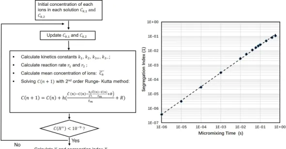
An algorithm has been built in Matlab to link the segregation index with micromixing time in a large range. Its procedure and the resulting relation between XS and tmunder the concentration
condition are shown in Fig.3. As a result, for each micromixing tests, the segregation index and the corresponding micromixing time can be quantified.
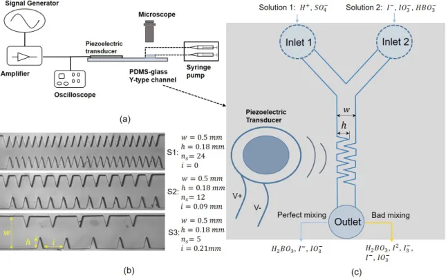
Figure 2 :Schematic of the experiment in this study: (a) experimental setup; (b) 3 different geom-etry structures tested, ns number of sharp edges on each side (c) Iodide-Iodate reaction within the
microchannel
3. Experiment setup and test procedure
3.1. Experiment setup
3.1.1. Y-type micromixer with piezoelectric transducer
A Y-shape mixer made of (Polydimethylsiloxane, PDMS) contains a Y-mixer and a channel with sharp-edge patterns.The preparation process using 2D photo-lithography on a wafer has been documented in our previous study, see Zhang et al. [1]. The PDMS microchannel is then sealed and stuck on a glass slide by oxygen plasma treatment. Three models (S1, S2, S3) are fabricated and their main geometrical dimensions are detailed in Fig.2 (b-c). Only the channel section with sharp edge patterns is shown, the Y-mixer being identical for all three models. To provide an acoustic field at a frequency range between 2 and 3 kHz, a piezoelectric transducer is stuck next to the channel on the glass slide. Streaming is then generated and characterized under various acoustic/flow conditions.
The experimental setup is shown in Fig.2 (a). The platform is composed of a syringe pump (Newtown Company & Co) allowing the injection of fluid from two syringes, under well-controlled flow-rate through the channel and via the two inlets. A function generator (Model 33220A Arbitrary waveform generator, Agilent) with a home-made adjustable power amplifier provides signal supply to the piezoelectric transducer (Model ABT-455-RC, RS Components). The transducer is glued on the glass microscope slide through which visualization is achieved by a binocular microscope together with a fast camera (MotionBLITZ Cube4, Mikrotron). The
piezoelectric transducer (diameter 35 mm and height 0.51 mm) delivers acoustic vibrations to the glass slide and to the whole channel stuck onto it, at various resonance frequencies from about 1 kHz up to 40 kHz. We chose to operate at one of these resonance peaks f , namely that at f =2.5 kHz. It turns out that the best operating conditions in terms of streaming flow were obtained at this frequency.
3.2. Experimental procedure
For the Iodide-Iodate reaction protocol, a spectrophotometer (Jenway 7310) is used to mea-sure the concentration of the I3− in the final solution. To adapt to the small throughput of the microchannel (Qc= 0 to 24 µL/min), we use a high-precision ultra micro-cuvette (Hellma,
QS105 model, 50 µL, light path 10 mm) to collect the solution after the reaction in the mi-crochannel. During the experiments, the cuvette is directly connected to the pipe out from the microchannel. And the measurement of the concentration is conducted as soon as the z-height is fully immersed by the effluents. To quantitatively analyze the micromixing process, Segre-gation Index and Micromixing time are determined through the IEM model. For each test, the concentration of I3−, measured by spectrophotometry, allows to determine Segregation Index and Micromixing time. The relation between XS and tm at given reactant concentrations is
shown later.
Besides the micromixing evaluation, visualisation of the macromixing between two fluids of different colors also helps tracing the mixing process. One fluid is formed by adding the blue dye into deionized water, while another one is pure colorless deionized water. The mixing processes of such two fluids in microchannel S2 are observed with the voltages from 10V to 40V.
3.3. Reactants and IEM modelling
The concentration of reactants are shown in Tab.1. It is obtained by trial and error since the appropriate concentration should give a concentration of I3− which drops in the range of the spectrophotometry (i.e., OD should fall between 0.1 and 3).
[H+] [KI] [KIO3] [N aOH] [H3BO3]
C [mol/L] 0.03 0.016 0.003 0.045 0.045
Table 1 :Concentration set to be used to characterize the mixing process
Micromixing time tm estimation characterizes the quality of micromixing process, which
can be compared even if the test is done with different initial concentration conditions. Repeat-ing the code described in Section 2.3. Interaction by Exchange with the Mean with different presumed tm, the corresponding XS can be obtained. Figure 3 shows the relation between XS
and tmunder the concentration conditions in this study.
4. Results and discussions
4.1. Acoustic streaming assisted macromixing
Streaming flow appears near multiple sharp edges once the piezoelectric transducer is acti-vated, as shown in the Fig. 4(a), which confirms our previous visualization results performed
Figure 3 :Step of algorithm for IEM and relation betweenXSandtm
to one single sharp edge (Fig.1(c)). These streamline are obtained by the tack of images taken at zero flowrate condition. It shows that fluid near the wall is jetted to the middle area of the microchannel while the previous fluid there is pushed back to the area between two edge struc-tures. Exchange between different areas is achieved by such acoustic streaming flow, which becomes a potential to reshape the interface line between two miscible flow and accelerate the mixing process between them. Figures 4 (b-f) illustrate the fluid mixing enhancement by acous-tic streaming at different intensities. The two fluids, discerned by dark and transparent colors, are fed through the two inlets through the Y-mixer. Inside the sharp-edge microchannel, as the voltages increase from the 10V to 40V, the interface turns from an approximately horizontal line (totally separated) to be irregular and blurred. When we focus on the first sharp edge (at the downside of the channel) encountered by incoming fluid, it is clear that at 30V or 40V, the dark fluid from the upside is sucked to the area near the tip and then jetted back to the middle area. In such situations, the contact between the two fluids strongly increases as soon as entering the sharp-edges area. Meanwhile, with higher voltages, the interface quickly blurs and disappears after several sharp edges. From the macroscopic perspective, the two fluids rapidly mix into each other while passing through the sharp-edges AS area.
4.2. XS and tmwith different Qcand structures
Figure 5 and Figure 6 show values of XS(left axis) and tm(right axis) according to input
volt-ages (thus magnitude of acoustic vibration), respectively from the three sharp-edge structures (S1/S2/S3) and flow-rate Qc. Firstly, as input voltage increase, XS and tm decrease quickly,
which means much better performance of mixing process is achieved. Taking S2 as an exam-ple, under acoustic streaming excitation, the segregation index decreases sharply from 0.06 (10 V) to 0.01 (40 V, good mixing). Micromixing time based on IEM decreases by a factor of 10: from 0.3s (10 V) to 0.04s with strong acoustic vibration (40 V). This trend corresponds to the macromixing images shown in Fig.4, namely with higher input voltage, interface between two different fluids is extended and mixing process at microscopic level is shortened. In terms of different sharp-edge structure S1/S2/S3, their influences on mixing have no obvious difference
Figure 4 :Mixing process intensified by different voltages between two miscible fluids (water, water with blue dye) using micromixer S2. (a): Acoustic streaming tracing from fluorescence particles tracking, at zero flowrate; (b): Static mixing effect without acoustic streaming, (0 V) and (c-f) Active mixing enhancement with acoustic streaming of different intensities (10-40 V). Flow from left to right,Qs= 4
µL/min.
at high input voltage while show distinct performance at low input voltage. The strength of more sharp edges inside the microchannel become prominent because of the weakness of single sharp structure at low input voltage.
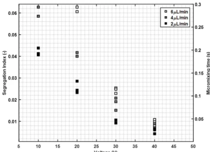
Another influential factor is the flowrate Qc. As shown in Fig.6, lower Qc through the
mi-crochannel corresponds to smaller XS and tm. This results are in accordance with our previous
study, namely the vortex formed by acoustic streaming near the sharp edge structure is sensitive to the throughput. This means, as throughput enlarges, the disturbance by streaming flow into the main flow decays quickly and results in worse mixing performance. Similarly, the differ-ences of values of XS and tm with different throughput are significant. Under weak acoustic
field and high throughput, the mixing improvement becomes weak or even negligible.
5. Conclusion
Acoustic streaming appears near multiple sharp-edges under low-frequency acoustic wave excitation. The disturbance by the streaming flow can accelerate the mixing process between two miscible flows. With a given microchannel, mixing performance depends on the input volt-age Vi, geometrical density of the sharp edge structures and throughput Qc. With Viincreasing
from 10V to 40V, XS and tmdecrease from 0.06 to 0.01 and 0.3 s to 0.04 s respectively,
achiev-ing much better micromixachiev-ing performance. In addition, the acoustic intensity (represented by input voltage Vi) seems to be the most significant influential parameter. At low acoustic
in-Figure 5 :Segregation IndexXS and
micromix-ing timetmwith different structures
Figure 6: Improvement of XSandtmdepends on
the channel throughputsQs
tensity Vi (10V), more sharp edges and lower throughput Qc are required to achieve low XS
and short tm. At higher acoustic intensities (Vi at 40V)), however, all three micromixers give
satisfactory micromixing effect.
References
[1] Zhang Chuanyu, Guo Xiaofeng, Brunet Philippe, Royon Laurent, Acoustic streaming near a sharp structure and its mixing performance characterization, Microfluidics and Nanofluidics., 104 (2019) 1613-4982.
[2] Ovchinnikov Mikhail, Zhou Jianbo, Yalamanchili Satish, Acoustic streaming of a sharp edge, The Journal of the Acoustical Society of America., 136 (2014) 22-29.
[3] Huang Po Hsun, Huang Po Hsun, Xie Yuliang, Ahmed Daniel, Rufo Joseph, Nama Nitesh, Chen Yuchao, Chan Chung Yu, Huang, Tony Jun An acoustofluidic micromixer based on oscillating side-wall sharp-edges, Lab on a Chip., 13 (2013) 3847-3852.
[4] Boluriaan Said, Morris Philip J. Acoustic Streaming: From Rayleigh to Today. Int. J. Aeroacoustics, 2003, 2, 255–292.
[5] Fournier M. C., Falk L. Villermaux J., A new parallel competing reaction system for assessing micromixing efficiency - Experimental approach, Chemical Engineering Science., 51 (1996) 5053-5064.
[6] Commenge Jean-Marc, Falk Laurent, Villermaux–Dushman protocol for experimental characteri-zation of micromixers, Chemical Engineering and Processing: Process Intensification., 50 (2011) 979-990.
[7] Guo Xiaofeng, Fan Yilin, Luo Lingai, Mixing performance assessment of a multi-channel mini heat exchanger reactor with arborescent distributor and collector, Chemical Engineering Journal., 227 (2013) 116-127.
[8] Villermaux Jacques, Falk Laurent, A generalized mixing model for initial contacting of reactive fluids, Chemical Engineering Science., 49 (1994) 5127-5140.
Acknowledgements
We would like to acknowledge the funding support from the CSC (China Scholarship Coun-cil).