Adaptive Realized Kernels

Texte intégral

(1)2011s-29. Adaptive Realized Kernels Marine Carrasco, Rachidi Kotchoni. Série Scientifique Scientific Series. Montréal Février 2011 – Version révisée le 4 mars 2013 February 2011 – Revised version on March 4, 2013. © 2011 Marine Carrasco, Rachidi Kotchoni. Tous droits réservés. All rights reserved. Reproduction partielle permise avec citation du document source, incluant la notice ©. Short sections may be quoted without explicit permission, if full credit, including © notice, is given to the source..

(2) CIRANO Le CIRANO est un organisme sans but lucratif constitué en vertu de la Loi des compagnies du Québec. Le financement de son infrastructure et de ses activités de recherche provient des cotisations de ses organisations-membres, d’une subvention d’infrastructure du Ministère du Développement économique et régional et de la Recherche, de même que des subventions et mandats obtenus par ses équipes de recherche. CIRANO is a private non-profit organization incorporated under the Québec Companies Act. Its infrastructure and research activities are funded through fees paid by member organizations, an infrastructure grant from the Ministère du Développement économique et régional et de la Recherche, and grants and research mandates obtained by its research teams. Les partenaires du CIRANO Partenaire majeur Ministère du Développement économique, de l’Innovation et de l’Exportation Partenaires corporatifs Banque de développement du Canada Banque du Canada Banque Laurentienne du Canada Banque Nationale du Canada Banque Royale du Canada Banque Scotia Bell Canada BMO Groupe financier Caisse de dépôt et placement du Québec Fédération des caisses Desjardins du Québec Financière Sun Life, Québec Gaz Métro Hydro-Québec Industrie Canada Investissements PSP Ministère des Finances du Québec Power Corporation du Canada Raymond Chabot Grant Thornton Rio Tinto State Street Global Advisors Transat A.T. Ville de Montréal Partenaires universitaires École Polytechnique de Montréal HEC Montréal McGill University Université Concordia Université de Montréal Université de Sherbrooke Université du Québec Université du Québec à Montréal Université Laval Le CIRANO collabore avec de nombreux centres et chaires de recherche universitaires dont on peut consulter la liste sur son site web. Les cahiers de la série scientifique (CS) visent à rendre accessibles des résultats de recherche effectuée au CIRANO afin de susciter échanges et commentaires. Ces cahiers sont écrits dans le style des publications scientifiques. Les idées et les opinions émises sont sous l’unique responsabilité des auteurs et ne représentent pas nécessairement les positions du CIRANO ou de ses partenaires. This paper presents research carried out at CIRANO and aims at encouraging discussion and comment. The observations and viewpoints expressed are the sole responsibility of the authors. They do not necessarily represent positions of CIRANO or its partners.. ISSN 1198-8177. Partenaire financier.

(3) Adaptive Realized Kernels Marine Carrasco *, Rachidi Kotchoni †. Résumé / Abstract Nous proposons un nouvel estimateur - les noyaux réalisés adaptatifs - pour la volatilité intégrée dans un cadre théorique combinant un modèle de volatilité stochastique avec effet de levier pour le prix d’équilibre de l’actif et un modèle semi-paramétrique spécifiée à la plus haute fréquence pour le bruit de microstructure. Avant de pouvoir implémenter les noyaux réalisés adaptatifs, certains des paramètres de dépendance temporelle du bruit de microstructure doivent d’abord être estimés. Nous étudions les performances de cet estimateur par simulation et illustrons son utilisation avec des données sur douze titres cotés dans le Dow Jones Industrial. Les résultats de simulation suggèrent que les noyaux adaptatifs réalisés permettent de faire un arbitrage optimal entre l’erreur de discrétisation et le bruit de microstructure. Mots clés : Bruit de microstructure, méthode des moments, noyaux adaptatifs réalisés, volatilité intégrée.. We design adaptive realized kernels to estimate the integrated volatility in a framework that combines a stochastic volatility model with leverage effect for the efficient price and a semiparametric microstructure noise model specified at the highest frequency. Some time dependence parameters of the noise model must be estimated before adaptive realized kernels can be implemented. We study their performance by simulation and illustrate their use with twelve stocks listed in the Dow Jones Industrial. As expected, we find that adaptive realized kernels achieves the optimal trade-off between the discretization error and the microstructure noise. Keywords: Integrated Volatility, method of moment, microstructure noise, realized kernel.. *. Université de Montreal - CIRANO - CIREQ. E-mail: [email protected] Visiting Scholar, Department of Economics - Université de Montréal, Address: C.P. 6128, succursale Centreville. Montréal, QC, H3C 3J7. Canada, Email: [email protected]. †.

(4) 1. Introduction. To estimate the monthly variance of a …nancial asset return, Merton (1980) proposes to use “the sum of the squares of the daily logarithmic returns on the market for that month with appropriate adjustments for weekends and holidays and for the no-trading e¤ ect which occurs with a portfolio of stocks”. Unfortunately, the daily data available to Merton does not span a long enough period for the purpose of his study. He circumvents this di¢ culty by using a moving average of monthly squared logarithmic return. In the same vein, French, Schwert and Stambaugh (1987) estimate the monthly variances by the sum of squared returns plus twice the sum of product of adjacent returns to correct for the …rst order autocorrelation bias. Andersen and Bollerslev (1998) are the …rst to support the empirical use of the realized volatility (RV) as an estimator of integrated volatility (IV) by a rigorous consistency argument taken from Karatzas and Shreve (1988). Since then, many authors including Jacod and Protter (1998) and Barndor¤-Nielsen and Shephard (2002) have well established the consistency of the RV for the IV when prices are observed without error. However, it is commonly admitted that recorded stock prices are contaminated with market microstructure noise. As pointed out by Andersen and Bollerslev (1998), “... because of discontinuities in the price process and a plethora of market microstructure e¤ ects, we do not obtain a continuous reading from a di¤ usion process...”. Barndor¤-Nielsen and Shephard (2002) show that in the presence of jumps that cause the price to exhibit discontinuities, the RV is consistent for the total quadratic variation of the price process. But the presence of noise in measured prices causes the RV computed with high frequency data to be a biased estimator of the object of interest. The sources of noise are discussed in Stoll (1989) and Hasbrouck (1993). In the words of Hasbrouck (1993), the “pricing errors” are mainly due to “... discreteness, inventory control, the non-information based component of the bid-ask spread, the transient component of the price response to a block trade, etc.”. Many approaches have been proposed in the literature to deal with the noise. One of them consists of sampling sparsely the high frequency returns so as to mitigate the impact of the noise su¢ ciently2 . Zhou (1996) and Hansen and Lunde (2006) propose a bias correction approach while Bollen and Inder (2002) and Andreou and Ghysels (2002) advocate …ltering techniques. Under the assumption that the volatility of the high frequency returns are constant within a day, Ait-Sahalia,. 3.

(5) Mykland and Zhang (2005) derive a maximum likelihood estimator of the IV that is robust to both IID noise and distributional misspeci…cation. Zhang, Mykland, and Ait-Sahalia (2005) propose another consistent estimator in the presence of IID noise which they called the two scale realized volatility. This estimator has been adapted in Ait-Sahalia, Mykland and Zhang (2011) to deal with dependent noise. Since then, other consistent estimators have become available among which the well-known realized kernels of Barndor¤-Nielsen et al. (2008a) and the pre-averaging estimator of Podolskij and Vetter (2009).3 This paper presents a general framework to design adaptive and e¢ cient kernel-based estimators for the integrated volatility in accordance with the properties of the noise. First, we propose a semi-parametric microstructure noise model that is tied to the frequency at which the price data are recorded. The noise is speci…ed as the sum of an endogenous term that is correlated with the e¢ cient returns and an exogenous term that is uncorrelated with the e¢ cient returns. Flexible restrictions are imposed on the exogenous noise so that it admits L-dependent and AR(1) dynamics as special cases. We superimpose the overall noise model to a stochastic volatility model with leverage e¤ect for the e¢ cient price. Second, we examine the implications of the overall framework for common realized measures that are aimed at estimating the IV. The bulk of the MSE of IV estimators is dominated by the contribution of the exogenous noise. When price data are contaminated with the endogenous noise only, the bias of the standard RV is O(1) while kernel-based estimators are unbiased and consistent. Under an MA(L) exogenous noise, realized Bartlett kernels with bandwidth larger than L are unbiased for the IV. When the exogenous noise is AR(1), an unbiased estimator of IV can be obtained only upon having a …rst step estimator of the noise autoregressive root in hand. If the …rst order autocorrelation of the exogenous noise converges to one as the record frequency goes to in…nity, then a necessary condition for the realized kernels to be consistent for the IV is that its bandwidth diverge su¢ ciently fast as the record frequency goes to in…nity. Third, we examine the trade-o¤ involved as one moves, on the one hand, from the standard RV to a bias-corrected RV, and on the other hand, from a bias-corrected RV to a consistent realized kernel. We show that unbiasedness and/or consistency are achieved by conceding more and more discretization error. Acting on this, we argue that the performance of any IV estimator at a given sampling frequency re‡ects the balance between the discretization error and the microstructure 4.

(6) noise at that frequency. We propose an adaptive realized kernel that achieves the optimal trade-o¤ bewteen both types of errors. As an optimal linear combination of initial estimators, the adaptive realized kernel provides us with an additional degree of freedom for tuning kernel-based estimators besides the bandwidth parameter. Fourth, we propose two inference procedures for the microstructure noise. The …rst procedure is designed for AR(1) types of noise and it is based on an overidenti…ed generalized method of moments. The second procedure is designed for MA(L) noises and it uses as many moment conditions as there are parameters to be estimated. The AR(1) assumption best suits for noise processes with in…nite dependence lag while the MA(L) assumption is reasonable if the noise has …nite dependence. Our simulations show that the inference procedure designed for AR(1) noises has good size and it has power against MA(L) alternatives. Hence, our best investigation strategy in practice consists of …rst testing whether the noise is AR(1) and next, applying the MA(L) inference procedure if the AR(1) speci…cation is rejected. We apply this strategy to twelve stocks listed in the Dow Jones Industrial and …nd that the AR(1) noise model cannot be rejected for six of them. For the other six stocks, we apply the MA(L) noise inference procedure and …nd estimates of L that lie between 8 and 12 minutes. The paper is organized as follows. In Section 2, we present our models for the frictionless price and for the microstructure noise. In Section 3, we study the properties of common realized measures within our framework. In Section 4, we design adaptive realized kernels for the IV. Our inference procedures for microstructure noise are presented in Section 5. In Sections 6 we evaluate the performance of all estimators proposed in the paper by simulation. Section 7 presents the empirical application and Section 8 concludes. The proofs are collected in an appendix.. 2. The Framework. First, we present a model for the e¢ cient price that allows for leverage e¤ect. Next, we present our model for the microstructure noise.. 5.

(7) 2.1. A Model for the E¢ cient Price. Let ps denote the latent (or e¢ cient) log-price of an asset and ps its observable counterpart. Assume that ps obeys the following stochastic di¤erential equation:. dps =. where. f. (s; ps ) ds +. s dWs ;. (:; :) is a deterministic and smooth function,. Brownian motion. In turn, assume that. d. s. s. s. satis…es:. =f(. s ) ds. +g(. p0 = 0;. (1). fs is a standard is the spot volatility and W s ) dBs ;. (2). where f (:) and g (:) are deterministic and smooth functions, Bs is a Brownian motion such that p 2 W , W is another Brownian motion that is independent of B and fs = Bs + 1 W 2 (0; 1) s s s is the leverage e¤ect parameter.. It is assumed that Equation (2) admits a continuous solution with in…nite lifetime so that any power function of the spot volatility process f Lebesgue Measure. Also, the processes. s gs 0. (s; ps ), f (. s). is locally integrable with respect to the and g (. s). are assumed adapted to the. …ltration generated by fWu ; Bu ; u < sg. Throughout this paper, it is maintained that there is no jump in the e¢ cient price. However, the conclusions of our analysis remain valid if a jump component that is uncorrelated with all other randomness is added to the e¢ cient price. In this case, the estimators that we consider for the IV are designed for the total quadratic variation of the e¢ cient price process.4 Without loss of generality, we condition all our analysis on the volatility path f. s gs 0. but the conditioning is often removed from the notation for simplicity. Accordingly,. all deterministic transformations of the spot volatility process are treated as constants. We assume that there exists a twice di¤erentiable deterministic function p(1) (:) that satis…es @p(1) ( s ) @ s. =. g(. s s). so that the stochastic process p(2);s = ps. p(1) (. s). follows a di¤usion without. leverage e¤ect5 . Indeed, by the Itô Lemma, we have:. dp(1);s =. (1);s ds. +. (1);s dBs ;. dp(2);s =. (2);s ds. +. (2);s dWs :. 6. and. (3) (4).

(8) where p(1);s. p(1) (. s ),. (1);s. =. s,. (2);s. =. p. 2. 1. s,. (2);s. 2 1 @ p(1) ( = f ( s) + g ( s) 2 @ 2 s. (1);s. =. s. s) 2. g (. (1);s. and. s) .. By construction, ps = p(1);s + p(2);s and p(1);s and p(2);s are uncorrelated. Hence, IVt = equal to the sum of the quadratic variations of p(1);s and p(2);s .. Rt. t 1. 2 ds s. is. We consider a sampling scheme where the unit period is normalized to one day. By de…nition, the microstructure noise is the di¤erence between the observed log-price and the e¢ cient log-price, that is, us = ps. ps . Thus, let rt denote the latent log-return at day t and rt its observable. counterpart. We have: rt where r(i);t =. Rt. t 1. pt. Rt (i);s ds + t 1. pt. = r(1);t + r(2);t + ut. 1. (i);s dWs .. ut. (5). 1. The drifts of the di¤usions (1), (3) and (4) are irrelevant. for their quadratic variations. Acting on this, we treat these di¤usions as though they had no drift (. s. =. (1);s. =. (2);s. = 0).. Suppose that we observe to a large number m of intradaily returns rt;1 ; rt;2 ; :::; rt;m for t = 1; :::; T days. We have: rt;j = r(1);t;j + r(2);t;j + ut;j where ut;j. ut. 1+j=m. Rt. 1+j=m t 1+(j 1)=m. and r(i);t;j. ut;j. 1. (i);s dWs .. for all t and j;. (6). It is maintained that the high frequency. observations are equidistant in calendar time. The noise-contaminated (observed) and true (latent) RV computed at frequency m are: (m). RVt. =. m X. 2 rt;j and RVt. (m). j=1. =. m X. rt;j2 :. j=1. Barndor¤-Nielsen and Shephard (2002) show that RVt. (m). converges to IVt and derived the asymp-. totic distribution: (m). RVt q P 2 3. IVt. m 4 j=1 rt;j. ! N (0; 1) ;. as m goes to in…nity. In the presence of microstructure noise, the estimator RVt. 7. (7). (m). is not feasible..

(9) 2.2. A Semiparametric Model for the Microstructure Noise. To model the microstructure noise, we posit that the frequency at which the price data are recorded determines the time series properties of the microstructure noise. This idea is acknowledge by Barndor¤-Nielsen et al. (2008a, Section 5.4 ) who considered “a situation where the serial dependence is tied to the sampling frequency [...], as opposed to calendar time”. Here, we follow a semiparametric approach that consists of specifying how the correlation structure of the noise changes as the record frequency increases. To motivate this approach, let us consider an MA(1) process "t;j at the highest frequency with E("2t;j ) = ! 0 and E("t;j "t;j. 1). frequency is m. By letting !. = ! 1 . The time elapsed between "t;j and "t;j h m; m. ! (0; m) = ! 0 ; !. is. h. h m. when the record. denote the h th order autocovariance of "t;j , we have: 1 ;m m. = ! 1 and !. h ;m m. = 0; h. 2:. (8). If we posit that "t;j remains an MA(1) with constant parameters whatever the record frequency, then we can assert that:. ! (0; km) = ! 0 ; !. 1 ; km km. = ! 1 and !. h ; km km. = 0; h. 2,. (9). as k ! 1 and m is …xed. However, if we assume that "t;j obeys an MA(1) model at the record frequency m but its …rst order autocorrelation is not invariant with respect to m, then (8) cannot be used to infer (9). By contrast, the autocorrelation structure of the sparsely sampled noise process can always be inferred from the properties of the noise at the highest frequency. With this in mind, we postulate the following microstructure noise model at the record frequency:. ut;j = at;j r(2);t;j + "t;j ; j = 1; 2; :::; m, for all t;. (10). where at;j is a time varying coe¢ cient that depends on the spot volatility process and "t;j is independent of the e¢ cient returns. In the words of Hasbrouck (1993), "t;j is the information uncorrelated or exogenous pricing error while at;j r(2);t;j is the information correlated or endogenous pricing error. We assume that time dependence in the noise process is only due to its information uncorrelated. 8.

(10) part. The following assumptions are further made: Assumption E0. at;j =. 0. +. p. , where. 1. m. 0. t;j. Z. 2 t;j. and. 1. t 1+j=m. t 1+(j 1)=m. are constants and:. 2 s ds:. Assumption E1. For …xed m, "t;j is a zero mean, discrete time and stationary process that is independent of f. sg. and rt;j .. Assumption E2. E2(a) E("t;j "t;j !. h m; m. h). !. h m; m. h m. = ! m;h , 0. 1 and ! m;h = 0 for all h > m, where. is bounded. E2(b) ! (0; m) = ! 0 for all m, and. ! m;h ! m;h+1 !0. = O(m. ) for some. 0, h = 0; :::; m. 1.. Assumption E3. For …xed m, we have: E3(a) E jut;j ut;j E3(b) V ar n. 4+ hj. 1=2 m. < 1, for some Pt0 +n Pm 1=2 t=t0 +1. > 0, for all h.. j=1 rt;j rt;j h. ! qh , uniformly in any t0 , as n ! 1.. Assumption E0 is a convenient way to depart from the constant coe¢ cient case (at;j =. 0). and. it implies that the variance of the endogenous part of the noise goes to zero at rate m:. V ar at;j r(2);t;j = 1. 2. 0 @. 2 0 t;j. +2. 0 1. s. 2 t;j. m. +. 1. 2 1A. m. :. Assumption E1 is quite standard in the literature. Assumption E2 stipulates general restrictions on the autocovariance structure of "t;j rather a parametric distribution. Assumption E2(a) imposes that "t;j be autocorrelated across j within the same day t, but not across days. This approximation is reasonable if the market closes at 4:30pm and re-opens the next day at 9:00am. Overall, Assumption E2 is consistent with several parametric models. An L-dependent model with …x lag L corresponds to. = 0 and ! m;h = 0 for all h > L. This includes the IID and uncorrelated noise as special cases.. One may also think of an MA(L) noise such that L = Cm for some constants C > 0 and case. =. = 0 brings us back to the MA(L) model with constant lag L whilst. 0. The. 2 (0; 1) describes a. situation where a higher market activity generates a noise with longer dependence lag.6 Assumption E2 also accommodates an AR(1) models. Indeed, assume that "t;j satis…es ! m;h = ! 0 ( and. m. =. ! m;1 !0 .. This model …ts into E2(b) if ! m;h 9. ! m;h+1 = ! 0 (. m). h. (1. m). = O(m. h m) ; h. 0. ), for all.

(11) h > 1. Hence, implies that. = 0 accommodates an AR(1) with constant autoregressive root whilst. m. 2 (0; 1). converges either to zero or to one as m ! 1.7. Finally, Assumption E3 replicates Assumption (1c) and Assumption 2 of Ubukata and Oya (2009) and it is needed for the central limit theorem of Politis, Romano and Wolf (1997) to hold. 2 is stationary and strong-mixing. This assumption is satis…ed if the squared return process rt;j. 3. Properties of Common Realized Measures. In this section, we study the traditional realized variance, the kernel-based estimator of Hansen and Lunde (2006) and the realized kernels of Barndor¤-Nielsen et al. (2008a) under our microstructure noise model.. 3.1. The Realized Volatility (m). Under an IID noise, RVt. is biased and inconsistent for IVt and its bias and variance increase. linearly in m, see e.g. Hansen and Lunde (2006). Here, we consider the sparsely sampled realized variance given by: (m ) RVt q. =. mq X k=1. with mq =. m q ;q. being the sum of q consecutive returns.8 Note that P = re(1);t;k + re(2);t;k where re(1);t;k = qk j=qk q+1 r(1);t;j and:. 1 and ret;k =. Equation (6) implies that ret;k re(2);t;k =. Pqk. j=qk q+1 rt;j. 1+ 0+ p m 0. with the convention that (mq ). variance of RVt. .. Pqk. 2 ; k = 1; :::; mq ; ret;k. +p. 1 t;qk. !. 1. m. 1 j=qk q+1 r(2);t;j. t;qk q. r(2);t;qk +. !. qk X1. r(2);t;j. j=qk q+1. r(2);t;qk. q. + ("t;qk. "t;qk. q) ;. = 0 when q = 1. The next theorem gives the bias and. Theorem 1 Assume that the noise process evolves according to equation (10). Then we have: (mq ). E RVt. = IVt +. 2mq (! 0 ! m;q ) {z } |. bias due to exogenous noise. 10.

(12) 2. +2 1 |. + 1 |. mq. (2 + 1) X + 1 p0 q m k=1 {z 2 1. t;qk. +. 0( 0. + 1). mq X. 2 t;qk. k=1. ! }. bias due to endogenous noise. 2. 2 0. 2 t;0. 2 t;m. {z. 2 + p0 1 m. t;0. t;m. end e¤ ects (mq ). V ar RVt. = O(mq ):. ; and }. The bias of RV (mq ) is comprised of three terms. The dominant term, 2mq (! 0 the exogenous noise. According to Assumption E2(b), this term is O(m1. ! m;q ), is due to. ) and hence. The second. term of the bias is due to the endogenous noise and it is O(1). The latter term does not diverge as m ! 1 and hence, a volatility signature plot may not be able to detect its presence. The third term of the bias is O(m. 1). and it is due to end e¤ects.. Gloter and Jacod (2001) considered an exogenous noise whose variance depends on the sampling frequency and they show that this noise is irrelevant if m times the noise variance is bounded for all m. Our endogenous noise satis…es this condition as it is Op (m. 1=2 ).. However, because it is. endogenous, it causes a bias term of magnitude O(1).. 3.2. The Estimator of Hansen and Lunde. Hansen and Lunde (2006) proposed the following ‡at kernel estimator:. (AC;m;L+1) RVt. =. m X. 2 rt;j. +. j=1. L+1 m XX. rt;j (rt;j+h + rt;j. h) ;. (11). h=1 j=1. (AC;m;L+1). where L is the dependence lag of the noise. When L = 0 so that "t;j is IID, RVt. coincides. with the estimator of French and al. (1987) and Zhou (1996): (AC;m;1) RVt. =. m X j=1. (AC;m;L+1). The estimator RVt. 2 rt;j. +2. m X. rt;j rt;j. j=1. 1. + (rt;m+1 rt;m rt;1 rt;0 ): {z } |. (12). end e¤ects. is unbiased for IVt under a general MA(L) noise. However, it is. biased if the exogenous noise is AR(1). An unbiased estimator under AR(1) exogenous noise is. 11.

(13) given by: (AC;m;1) RVt. =. m X. 2 rt;j. +. j=1. where. m. m X. rt;j (rt;j+1 + rt;j. 1). j=1. +. m X. 1 1. rt;j (rt;j+2 + rt;j. 2). (13). m j=1. is the autoregressive root of the noise.9 In order to gain some insights on the properties. of the estimators above, we specialize the exogenous noise to the IID case and derive the mean and (AC;m;1). variance of RVt. .. Theorem 2 Assume that the noise process evolves according to Equation (10). If "t;j is IID, then we have: (AC;m;1). E RVt. = IVt + 1. (AC;m;1). V ar RVt. h. 2. = O (m) :. 2 0. +2. 2 t;m. 0. 2 t;0. 2. (1+ 0 ) 1p m. t;m. t;0. i. ; and. When the endogenous noise is absent and the exogenous noise is IID, Theorem 2 yields a well(AC;m;1). known result derived by Hansen and Lunde (2006, Lemma 3). In this particular case, RVt. (AC;m;L+1). is unbiased for IVt while its variance increases linearly in m and consequently, RVt (AC;m;1). RVt. and. are not consistent for IVt .. When the exogenous noise is absent so that the noise is purely endogenous, it can be shown that (AC;m;1). the bias and variance of RVt. are both O m. 1. . This result is obtained by specializing the. formulas derived in the proof of Theorem 2 to the "no leverage and no exogenous noise" case. Hence, (AC;m;1). RVt. is consistent for IVt in the presence of the endogenous noise. This property extends to. (AC;m;L+1). RVt. (AC;m;L+1). since RVt. (AC;m;1). The same can be said for RVt. (AC;m;1). RVt. converges to zero in the absence of exogenous noise.. as long as an estimator of. m. that converges su¢ ciently fast. is available. (AC;m;L+1). The realized kernel considered in the next section is a version of RVt. where the higher. order covariance terms are weighted by a kernel function. Hence, this estimator is also robust to endogenous noise and leverage e¤ect. Acting on this, we study the realized kernel below by assuming that. 0. =. 1. =. = 0.. 12.

(14) 3.3. The Realized Kernels. Barndor¤-Nielsen et al. (2008a) proposed the following estimator for IVt which they named “realized kernel ”: KtBN HLS =. t;0 (r) +. H X. h. k. 1. t;h (r). H. h=1. +. t; h (r). for a positive kernel function k (:) such that k (0) = 1 and k (1) = 0, where. ;. t;h (x). (14) =. Pm. j=1 xt;j xt;j h. for any variable x. Equation (14) is reminiscent of the long run variance estimators of Newey and West (1987) and Andrews and Monahan (1992). Barndor¤-Nielsen et al. (2008a, Proposition 3 ) show that KtBN HLS is consistent for IVt for some choices of bandwidth if the covariance between "t;h and "t;h This condition is satis…ed for an AR(1) noise with. m. vanishes for any h and j as m ! 1.. ! 0 as m ! 1 or for an MA(L) noise with. constant lag L. It is not satis…ed for an AR(1) noise with noise with L = Cm and. j. m. ! 1 as m ! 1 nor for an MA(L). > 0. For the latter MA(L) noise, Assumption E2(b) implies that:. ! m;j. !0 =. j 1 X. (! m;h. ! m;h+1 ) = O(jm. ):. h=0. Hence, ! m;j. ! 0 = O(m. ! m;j m!1 ! 0. ) and lim. = 1 for any …xed j.. Further, Barndor¤-Nielsen et al. (2008a, Proposition 4 ) show that KtBN HLS is consistent for IVt when "t;j is AR(1) with constant autoregressive root. Below, we study the estimator given by:. BN HLS Kt;Lead. =. t;0 (r). +2. H X h=1. k. h. 1 H. s;h (r) ;. (15). when the …rst order autocorrelation of the noise converges to one as m ! 1 and we use the results BN HLS can be decomposed as: to infer some properties of KtBN HLS . Note that Kt;Lead. BN HLS Kt;Lead = Kt (r ) + Kt (r ;. 13. u) + Kt ( u; r ) + Kt ( u) ;.

(15) where. Kt (x) =. t;0 (x). Kt (x; y) =. +2. t;0 (x; y). H X. h. k. h=1 H X. +2. 1. h. k. t;h (x; y). =. noise.. Pm. j=1 xt;j yt;j h .. Theorem 3 Assume that. 0. =. 1. t;h (x; y) ;. H. h=1. and. t;h (x) ;. H. We have the following consistency result under IID exogenous. =. 1. = 0, k (x) = 1. x (the Bartlett kernel) and "t;j is IID.. Then, we have: BN HLS Kt;Lead. IVt =. "2t;0 + "2t;m + Op (m. 1=6. ):. as m ! 1 and H is proportional to m2=3 . Barndor¤-Nielsen et al. (2008a, Theorem 4) gives the same rate of convergence for KtBN HLS BN HLS . Note that K BN HLS = under the conditions of Theorem 3. Here, Theorem 3 focuses on Kt;Lead t 1 2. BN HLS + K BN HLS Kt;Lead t;Lag. BN HLS is the twin estimator given by: where Kt;Lag. BN HLS Kt;Lag =. t;0 (r) + 2. H X. h. k. H. h=1. BN HLS Hence, V ar Kt;Lead. 1. s; h (r). is always larger than V ar KtBN HLS although both estimators enjoy the. same rate of convergence. BN HLS have the same When the noise is not IID but remains purely exogenous, KtBN HLS and Kt;Lead. expectation as Kt ( u). We have the following results. Theorem 4 Assume that. 0. =. 1. =. = 0, k (x) = 1. x (the Bartlett kernel) and "t;j and that. Assumptions E1 and E2 hold. (i) If the noise is AR(1) with autoregressive root. E (Kt ( u)) =. If further. m. '1. Dm. (. 0) so that. 2mH. m. 1. m,. (. then we have:. H m). (2 +. m) !0:. ! 1 as m ! 1 and H = Cm ( 2 (0; 1)) then we 14.

(16) have: jE (Kt ( u))j ' 2 (2 +. 1 m ) ! 0 Cm. exp. (ii) If the noise is MA(L), E (Kt ( u)) = 0 as long as H. CDm L + 1.. The …rst result of Theorem 4 stipulates that under an AR(1) exogenous noise with m ! 1, E (Kt ( u)) converges to zero if and only if H = Cm with. ! 1 as. m. > . Otherwise, the bias. diverges to in…nity. Hence, a necessary condition for the MSE of KtBN HLS to be …nite is that H diverges to in…nity su¢ ciently fast as m ! 1. Under MA(L) noise, E (Kt ( u)) = 0 if H is greater than the dependence lag of the noise. Again, if L = Cm as assumed, a su¢ cient condition for KtBN HLS to be unbiased is that H diverges to in…nity faster than L as m ! 1.. 4. Adaptive Realized Kernels. The results of a simulation study performed by Gatheral and Oomen (2007) suggests that incon(AC;m;1). sistent estimators like RVt. often outperform some theoretically consistent estimators like. KtBN HLS at record frequencies commonly encountered in practice (e.g. one to …ve minutes). From (AC;m;1). a theoretical point of view, one can think of at least three situations where the MSE of RVt. can be lower than that of KtBN HLS . The …rst situation is the one in which the variance of the microstructure noise is so small that it contributes very little to the MSE. The second situation may happen because the bandwidth H is not optimally selected for KtBN HLS . The third situation corresponds to the case where the sampling frequency is not large enough to make the asymptotic results for KtBN HLS useful. All three situations are related to the fact that the performance of an IV estimator at a given sampling frequency re‡ects the trade-o¤ between the discretization error and the (AC;m;1). microstructure noise at that frequency. Indeed, RVt (m). RVt. is exempted of the bias of its ancestor. at the expense of a higher discretization error (i.e. the MSE in the absence of noise). Also, (AC;m;1). KtBN HLS brings consistency upon conceding a higher discretization error than RVt. . Given. that the discretization error KtBN HLS increases with the bandwidth H, the optimal selection of H involves a trade-o¤ between the MSE due to discretization and the MSE due to the microstructure noise. Below, we propose an adaptive estimator that is aimed at achieving this optimal trade-o¤.. 15.

(17) Consider N kernel-based estimators of IVt given by: c (i) = IV t. t;0 (r) +. H X. ki. h. 1. t;h (r). H. h=1. +. t; h (r). ; i = 1; 2; :::; N;. (16). where ki (:) ; i = 1; :::; N are distinct kernel functions. Alternatively, one may consider using the same kernel function but di¤erent bandwidths, as in the following example: c (i) IV t =. t;0 (r) +. Hi X. k. h. 1. t;h (r). Hi. h=1. +. t; h (r). ; i = 1; 2; :::; N:. By letting H = max H1 , the latter equation may be re-written as (16) with ki (x) 1 i N. x. k. H Hi x. ;0. 1 and ki (x) = 0 otherwise. We consider selecting the estimator with smallest MSE within the class de…ned by:. Kt$ =. N X i=1. c (i) subject to $i IV t. N X. $i = 1;. i=1. where $ = ($1 ; :::; $N )0 is a vector of weights. Note that Kt$ is also a realized kernel, as we have: Kt$ =. t;0 (r) +. H X. k$. h=1. with k$ (x) =. h. 1 H. t;h (r). +. t; h (r). ;. (17). PN. i=1 $ i ki (x).. To illustrate the idea, suppose that the exogenous noise is L-dependent. Then, we may de…ne: Kt$ = (1. (1). (2). c t + $IV ct ; $) IV. c (1) c (2) where IV is KtBN HLS at bandwidth L and IV is the same estimator at bandwidth H. We t t have:. Kt$. =. t;0 (r). +. L+1 X h=1. k. h. 1 H. t;h (r). +. t; h (r). +$. H X. h=L+2. k. h. 1 H. t;h (r). +. t; h (r). We see that Kt$ exploits the L-dependence of the noise by discounting the kernel windows assigned to the covariance terms beyond lag L + 1. The optimal weight $ that minimizes the MSE of. 16.

(18) Kt$ mitigates the impact of the discretization error induces by the higher order covariance terms while guaranteeing that Kt$ inherits the consistency of KtBN HLS . The standard realized kernel includes the covariance terms of higher displacements in order to control the variance, but it does not exploit the life of a dependent noise. A theoretical importance of the estimator Kt$ resides in that it introduces an extra degree of freedom ($) besides the bandwidth parameter (H) and hence, it provides an adaptive approach for tuning realized kernel. Subsequently, we refer to Kt$ as the “adaptive realized kernels”. Note that Kt$ has the ‡avor of a model averaging estimator (see Hansen, 2007) and it shares some similarities with the estimator proposed in Ghysels, Mykland and Renault (2008). Let Vbt =. c (1) ; :::; IV c (N ) IV t t. 0. so that Kt$ = $0 Vbt with $0 = 1, where IVt )2 = $0 $, where. unconditional MSE of Kt$ is E (Kt$. =E. is a vector of ones. The. Vbt. IVt. the MSE matrix of the vector Vbt . The optimal vector of weights is given by: $ =. 0. 1. 1. Vbt. 1. IVt. 0. is. (18). A feasible vector of weights is obtained by plugging an empirical counterpart of. into (18), as. illustrated in Section 6.2. By construction, the MSE of Kt$ is necessarily smaller than the MSE of c (i) ; i = 1; :::; N . each of the initial estimators IV t. 5. Inference on the Microstructure Noise Parameters. In order to implement the realized kernels e¢ ciently, one needs to know whether the noise has …nite dependence lag or in…nite dependence lag. In this section, we consider estimating the correlogram of the noise by assuming that the noise is either AR(1) or MA(L) at a given record frequency m.10 The AR(1) assumption targets noises with in…nite dependence lag while the MA(L) assumption provides a reasonable approximation if the noise has …nite dependence. From Theorem 2, we can infer that:. E. t;1. =. 1. 2. m X. 0. j=1. +m ( ! 0 + 2! m;1. +p. 1. m. t;j 1. ! m;2 ) ;. 17. !. 1+. 0. +p. 1. m. t;j 1. !. 2 t;j 1.

(19) where. t;h. (m). is used as shorthand for. t;h (r). Let bt. h (m) = E RVt. i IVt denote the bias of the. realized volatility computed at the record frequency. When q = 1, it follows from Lemma 5 in appendix that: (m) bt. 2. = 2 1. m X. 0. j=1. +2m (! 0. +p. 1. m. t;j 1. ! 2 0. 2. ! m;1 ) + 1. 1+. 0. 2 t;0. +p 2 t;m. 1. m. t;j 1. !. 2 t;j 1. 2 + p0 1 m. t;0. t;m. :. Hence, the following unconditional moment conditions hold: (m). E RVt. E. E. t;1. t;h+1. +. +. (m). = IVt + bt (m). ;. t; 1. =. bt. t; h 1. =. 2m (! m;h. (19). + 2m (! m;1. ! m;2 ) and. (20). 2! m;h+1 + ! m;h+2 ) ; h. 1;. (21). Below, we consider the AR(1) and MA(L) cases separately.11. 5.1. Inference with an AR(1) Microstructure Noise. Under an AR(1) model, the noise autocovariances satisfy ! m;h = ! 0 ( implies that E (b gh (! 0 ;. m )). h m). and thus, Equation (21). = 0 with:. T 1 X gbh (! 0 ; m ) = 2mT. t;h+1. +. t; h 1. + ! 0 (1. m). 2. (. m). h. ,h. 1. (22). t=1. Let gb = (b g1 ; :::; gbn ) be a vector of n selected moments conditions, with gbh estimators of (! 0 ;. m). are given by:. ! b0 b. m. = arg min gb0 Sb. 1. gbh (! 0 ;. m ).. The GMM. gb;. where Sb is a consistent …rst step estimator of the long run covariance matrix of the moment condip tions, that is, Sb = lim V ar T gb . T !1. After estimation, the overidenti…cation test of Hansen (1982) may be used to check whether. the AR(1) model …ts the data reasonably well. This test is based on the following asymptotic. 18.

(20) distribution under the null hypothesis that the AR(1) model is true: J = T gb0 Sb. 1. 2. gb !. (N. 2) as T ! 1;. (23). After performing this test, and if the null hypothesis is not rejected, we may then perform a standard t-test for the signi…cance of the parameters (! 0 ;. m ).. The distribution of the estimators under the. null hypothesis is: p. ! b0 T b. !0. m. m. 0 ; G0 Sb 0. !N. 1. G. 1. :. (24). 2) Jacobian matrix of the moment conditions. The hth row of G is given by:. where G is the (n. @b gh @b gh ; @! 0 @ m. Gh = =. (1. 2 h m) ( m) ;. h m) ( m). 2! 0 (1. + h! 0 (1. m). 2. (. m). h 1. Note that G is a deterministic matrix.. 5.2. Inference with an MA(L) Microstructure Noise. Under the MA(L) model, the noise autocovariances satisfy ! m;h = 0 for h > L. Thus, Equations (19)-(21) provide L + 2T moment conditions that can be used to estimate L + 2T parameters, n oT (m) namely bt ; IVt and f! m;h gL h=1 . Estimating these parameters by the method of moments is t=1. straightforward. First solving for ! m;L and then proceeding by backward substitution into (21) to (m). (19) yields the following unbiased estimators for ! m;h , bt. ! b m;h = bb(m) = t. (AC;m;L+1). RV t. T L h+1 1 X X l 2T m s=1. t;1. +. s; h l. ; h = 1; :::L;. (25). l=1. T L+1 1 XX T. t; 1. s;l. +. s; l. and. (26). s=1 l=2. (m). = RVt =. s;h+l. and IVt respectively:. t;0 +. bb(m) t. t;1 +. (27) t;. 1+. T L+1 1 XX T s=1 l=2. 19. s;l. +. s; l. :.

(21) (AC;m;L+1). (AC;m;L+1). Hence, RV t. is an unbiased method-of-moment estimator of IVt . Note that RV t. specializes to the estimator of Hansen and Lunde when T = 1. To estimate the noise variance ! 0 , we use the expression of the bias of the RV sampled at the highest frequency. We have: T 1 X b(m) ! b0 = bt + ! b m;1 2mT. (28). t=1. All the noise autocovariance estimates can be written as:. ! b m;h. T m 1 XX = ! b t;j;h ; h = 0; 1; :::; L mT. where ! b t;j;h , h = 0; :::; L are de…ned as follows: ! b t;j;0 =. (b ! t;j;1 ; :::; ! b t;j;L )0 = P t;j;(2;L+1). with. t;j;h. = 12 rt;j (rt;j. Pi;i+1 = 2, Pi;i+2 = of the vector P. 1. h. (29). t=1 j=1. =. L+1 1X 2. t;j;h. +. h=1 1 t;j;(2;L+1). t;j;2 ; :::;. t;j; h. + P. 1. t;j;(2;L+1). 1. ,. and. t;j;L+1. 0. :. + rt;j+h ) for all t and h, P being the L L matrix with elements: Pi;i =. 1; Pi;j = 0 otherwise 1. i; j. L, and P. 1. t;(2;L+1). 1. 1,. being the …rst element. t;(2;L+1) .. b h given by: Based on Equation (29), we consider the subsampled variance Q bh = Q. T mX. T. t=1. 0. m X @1 ! b t;j;h m j=1. 12. ! b m;h A :. (30). Under Assumptions E1, E2 and E3, we have: (mT )1=2 (b ! m;h q bh Q. ! m;h ). ! N (0; 1). (31). as T goes to in…nity and m is …xed. See Ubukata and Oya (2009) for the proof.12 The knowledge of L is required to estimate the correlogram of the microstructure noise. A simple way to estimate L is to perform signi…cance tests for ! m;h by using autocovariance estimates. 20.

(22) that rely on an initial guess Lmax .13 Under the null hypothesis that ! m;h = 0, we have:. bh =. (mT )1=2 ! b m;h q ! N (0; 1) bh Q. (32). b is the maximum lag at which the The statistics bh diverges under the alternative. The estimator L. ^ null is rejected. Provided that the initial guess Lmax exceeds the true value of L, the estimator L will not underestimate the true L asymptotically.. 6. Monte Carlo Simulations. The simulation study is organized as follows. First, we apply the AR(1) noise inference procedure to a correctly speci…ed model. Second, we verify the power of this procedure by applying it to an MA(3) noise. Third, we study the performance of the MA(L) noise inference procedure when the model is correctly speci…ed. Finally, we assess the quality of the IV estimators under either type of noise.. 6.1. The Data Generating Processes. We assumed that the e¢ cient log-price process evolves according to the model of Heston (1993):. dpt. =. 2 t. =. d. t dW1;t. and 2 t. dt +. (33) t. dW1;t +. p 1. 2 dW. 2;t. where W1;t and W2;t are independent Brownian motions and the parameter. ;. (34). captures the leverage. e¤ect. Following Zhang and al. (2005), we set the annualized parameters values as follows:. = 5;. = 0:04;. = 0:5; 2 f0; 0:5g ;. Using the Poisson-Mixing-Gamma characterization of Devroye (1986) for the spot volatility process (34), we simulate the e¢ cient price data at …ve seconds14 but we assume that the record frequency is one minute. To start with, we simulate once and for all a sample of T = 500 days of e¢ cient price data. Next, 21.

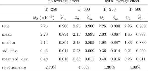
(23) we contaminate iteratively this sample with a microstructure noise that is simulated according to:. ut;j =. where. 0. = 0:5;. 1. 0. +p. !. 1. m. t;j. = 0:5 and the exogenous noise "t;j is either an AR(1) or an MA(3). For the. AR(1) exogenous noise, we use "t;j =. m "t;j 1. and. 0. 0. rt;j + "t;j , j = 1; :::; m;. varying so as to match ! 0 =. ! 0 2 2:5 The variance ! 0 = 2:5. 7. 10. frequency while ! 0 = 2:25. 2 m). 1 (. 10. 7. + vt;j , with vt;j. IID. N (0;. 0 );. m. 2 f 0:9; 0; 0:9g. with the following values:15. ; 2:25. 6. 10. ; 2:5. 10. 5. :. (35). has been used in Zhang and al. (2005) at …ve minute sampling 6. 10. has served in Ait-Sahalia and al. (2005) at frequencies ranging. from one to thirty minutes. For the MA(1) exogenous noise, we use "t;j = vt;j + N (0;. 0 ),. 1. = 0:5,. 2. = 0:2 and. !0. where. 6.2. 0. 3. 1 vt;j 1. +. 2 vt;j 2. +. 3 vt;j 3 ,. with vt;j. IID. = 0:05. This implies:. E "2t;j =. 0. 1+. 2 1. +. 2 2. +. 2 3. +. ! m;1. E ("t;j "t;j. 1). =. 0( 1. +. 1 2. ! m;2. E ("t;j "t;j. 2). =. 0( 2. +. 1 3). ! m;3. E ("t;j "t;j. 2). =. 0 3. ! m;h. E ("t;j "t;j. h). = 0 for all h. = 0:05. 0. = 1:2925 2 3). = 0:225. 0;. = 0:61. 0;. 0;. and. 4;. varies so as to match the variances in (35).. Simulation Results. Table 1 presents the estimation results for a correctly speci…ed AR(1) noise model. The simulations are performed with and without the leverage e¤ect.. Table 1: Estimation of a well-speci…ed AR(1) noise model by GMM m. = 0:9, m = 390, 1000 replications. 22.

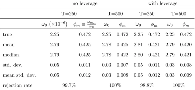
(24) no leverage e¤ect T=250 ! b0. true. 10. 6. with leverage e¤ect. T=500 b. m. ! b0. b. m. T=250 ! b0. b. m. T=500 ! b0. b. m. 2:25. 0:900. 2:25. 0:900. 2:25. 0:900. 2:25. 0:900. mean. 2:20. 0:894. 2:15. 0:895. 2:03. 0:887. 1:85. 0:883. median. 2:14. 0:894. 2:13. 0:895. 1:98. 0:887. 1:83. 0:883. std. dev.. 0:43. 0:014. 0:28. 0:009. 0:36. 0:014. 0:21. 0:009. mean std. dev.. 0:48. 0:016. 0:33. 0:011. 0:40. 0:015. 0:25. 0:011. rejection rate. 2:70%. 4:00%. 1:30%. 4:00%. We see that the estimators ! b 0 and bm are slightly biased downward. The bias is more pronounced. in the presence of leverage e¤ect and it is more visible for ! b 0 .16 The standard deviation (std. dev.) of the empirical distribution of the estimates is quite close to the mean of the standard deviations. (mean std. dev.) implied by the analytical formula (24). The last row of the table gives the rate of rejection of the null hypothesis that the true model is AR(1) by the overidenti…cation test at nominal level 5%. Overall, the results suggest that the overidenti…cation test has good size. In order to assess the power of the previous test, we …t an AR(1) model to an MA(3) microstructure noise. Table 2 presents the results of the simulation. The …rst order autocorrelation of the MA(3) noise gives us a pseudo-true value for. m.. In all the scenarios, the noise variance is. overestimated while the …rst order autocorrelation is underestimated. The model rejection rate is nearly 100%, which indicates that the overidenti…cation test has power against MA(L) alternatives. Acting on these results, our preferred strategy for the empirical investigation will consist of …rst testing the null hypothesis that the noise is AR(1) and next, estimating an MA(L) noise if the AR(1) assumption is rejected.. Table 2: Estimation of a misspeci…ed AR(1) noise model True model is MA(3), m = 390, 1000 replications. 23.

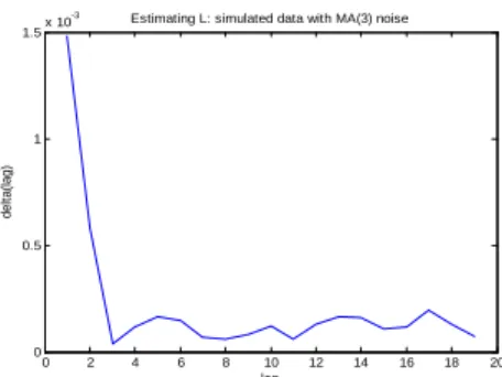
(25) no leverage. with leverage. T=250 !0. 6. 10. T=500. m. ! m;1 !0. !0. T=250 !0. m. T=500 !0. m. m. true. 2:25. 0:472. 2:25. 0:472. 2:25. 0:472. 2:25. 0:472. mean. 2:79. 0:425. 2:78. 0:425. 2:81. 0:421. 2:79. 0:420. median. 2:79. 0:425. 2:78. 0:422. 2:80. 0:421. 2:79. 0:421. std. dev.. 0:05. 0:011. 0:03. 0:007. 0:05. 0:011. 0:03. 0:008. mean std. dev.. 0:05. 0:012. 0:03. 0:008. 0:05. 0:012. 0:03. 0:009. rejection rate. 99:7%. 100%. 98:8%. 100%. We now study the performance of the inference procedure outlined previously for an MA(L) noise. The …rst step consists of guessing an initial value Lmax that is larger that the true dependence lag L. We use an heuristic based on the following empirical MSE: T 1X (l) = KtT T. (AC;m;l) 2. RV t. t=1. (AC;m;l+1). where RV t. ; l = 1; :::; b2H=3c. (AC;m;1). is de…ned as in (27), KtT = RVt. + T1. PT. s=1. PH. h=2. and it is implicitly assumed that H is large enough to ensure that L (AC;m;l). RV t. (AC;m;L+1). is obtained by truncating the formula of RV t. thus, it is thus unbiased for IVt when l (AC;m;H). RV t. 1. (36). h 1 H. s;h. +. s; h. b2H=3c. On the one hand,. to l autocovariance terms and. L + 1. On the other hand, KtT is a smoothed version of. and it is also unbiased for IVt if the bandwidth H is selected su¢ ciently large. Hence. the mean of KtT. (AC;m;l). RV t. Also, the variance of KtT. is decreasing in l as l increases to L and it is equal to zero for l (AC;m;l). RV t. is increasing in l. As a result, the curve of. L+1.. (l) is L-shapped. e of L is given by the point where the curve (l; (l)) is bent the or convex. An initial estimate L most or by the minimum of that curve. Figure 1 shows an L-shapped example with an MA(3) noise. e and L b coincide with Table 3 shows the simulation results for the estimation of L. The medians of L. the true value L = 3. The corresponding means are slightly biased downward, but this is repaired by rounding up the estimates to the next unit. Figure 1: Plots of. (l) against l. An example with an MA(3) noise.. 24.

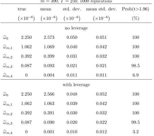
(26) -3. 1.5. Estimating L: simulated data with MA(3) noise. x 10. delta(lag). 1. 0.5. 0. 0. 2. 4. 6. 8. 10 lag. 12. 14. 16. 18. 20. Table 3: Estimation of the dependence lag L True model is MA(3), m = 390, T = 250, 1000 replications. ! 0 = 2:25. e L. b L. 6. 10. ! 0 = 2:5. 10. 5. no leverage. with leverage. no leverage. with leverage. min. 2:00. 2:00. 2:00. 2:00. mean. 2:97. 2:91. 2:99. 2:99. median. 3:00. 3:00. 3:00. 3:00. max. 3:00. 3:00. 3:00. 3:00. min. 2:00. 2:00. 2:00. 2:00. mean. 2:61. 2:63. 2:90. 2:91. median. 3:00. 3:00. 3:00. 3:00. max. 3:00. 3:00. 3:00. 3:00. e + 3 for the estimation of the correlogram of the noise. Table 4 presents Below, we use Lmax = L. the results. Note that the estimator of ! 0 is expected to be biased upward because it re‡ect the size of the total noise contaminating the e¢ cient price. Indeed, we have:. E (b !0). !0 = 1. 2. 2 1. m. +. 1 (2 0. p. + 1) E m. t;qk. +. 0( 0. + 1) E. 2 t;qk. :. The results suggest that the autocovariances f! l g4l=1 are estimated without bias. The mean standard deviation (mean std. dev.) is the average of the standard deviations implied by the analytical formula (30). Interestingly, the average of the standard deviations obtained by the analytical formula is close to the empirical standard deviation of the simulated estimates. The last column gives the rate of rejection of the null hypothesis that ! h = 0. It appears that a standard t-test for the null hypothesis 25.

(27) ! 4 = 0 has a good size at 5% nominal level. Also, the separate tests for the null hypotheses ! h = 0 have power against the alternatives ! h 6= 0; h = 1; 2; 3.. Table 4: Estimation of the Correlogram of the noise. m = 390, T = 250, 1000 replications true 10. mean 6. 10. std. dev. 6. 10. mean std. dev.. 6. 10. Prob(t>1.96). 6. (%). no leverage ! b0. ! b m;1. ! b m;2. ! b m;3. 2:250. 2:573. 0:050. 0:051. 100. 1:062. 1:069. 0:040. 0:042. 100. 0:392. 0:399. 0:031. 0:032. 100. 0:087. 0:093. 0:021. 0:021. 98:5. 0. 0:004. 0:011. 0:011. 6:9. ! b m;4 ! b0. ! b m;1. ! b m;2. ! b m;3. with leverage 2:250. 2:566. 0:048. 0:052. 100. 1:062. 1:063. 0:039. 0:042. 100. 0:392. 0:391. 0:030. 0:032. 100. 0:087. 0:090. 0:020. 0:022. 99:5. 0. 0:001. 0:010. 0:012. 3:2. ! b m;4. As a …nal step of this simulation study, we evaluate the performance of the adaptive realized P c (i) c (1) kernels Kt$ by simulations. Under either type of noise, we set Kt$ = 4i=1 $i IV t , with IV t = BN HLS , IV c (2) = K BN HLS , IV c (3) = K BN HLS and IV c (4) = K BN HLS , where K BN HLS is the Kt;15 t t t t;25 t;35 t;45 t;H. c (1) c (2) c (3) c (4) IV t ; IV t ; IV t ; IV t. realized Bartlett kernels with bandwidth H. Let Vbt = noise, the MSE matrix of Vbt is B=. 0. . Under AR(1). = V ar Vbt + BB 0 , where B is the 4x1 vector of biases given by:. 2m! 0 (2 +. m). (. m). 15. 15. ;. (. 25 m). 25. ;. (. m). 35. 35. ;. (. m). 45. 45. !0. (37). and V ar Vbt is the covariance matrix of Vbt . Note that the expression of the bias is deduced from. Theorem 4. When the noise is MA(3), the bias vector is B = (0; 0; 0; 0)0 and the MSE reduces 26.

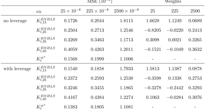
(28) to. = V ar Vbt . In order to simplify the steps of the Monte Carlo simulation, we assume the. ideal situation where ! 0 ,. m. and L are known (in the empirical application, these parameters are by replacing V ar Vbt by its sample counterpart:. replaced by their estimates). We estimate. Vd ar Vbt. T 1X b = Vt T t=1. T 1X Vl T l=1. !. T 1X Vl T. Vbt. l=1. !0. (38). The MSE of each IV estimator reported in the tables is computed as: T (i) 1 X c (i) c M SE(IV t ) = IV t T. 2. IVt. , i = 1; :::; 4. t=1. where IVt is inferred from the simulated volatility path at one second frequency. Table 5 shows the simulation results under IID noise, with and without leverage e¤ect. We see that the MSE of all IV estimators are slightly smaller in the presence of leverage e¤ect compared to when there is no leverage. Otherwise, the simulation results are qualitatively similar. When the noise variance is small (! 0 = 25. 10. 8 ),. BN HLS ) has the estimator with smallest bandwidth (Kt;15. the smallest MSE and it is assigned the largest weight in the design of the adaptive estimator Kt$ . By contrast, when the noise variance is large (! 0 = 2500. 10. 8 ),. BN HLS is the most e¢ cient Kt;35. estimator and it receives the largest or the second largest weight. In either case, the estimator with BN HLS ) is not e¢ cient because it does not optimally balance the discretization largest bandwidth (Kt;45. error against the microstructure noise. As expected, the adaptive realized kernel is more e¢ cient than all other estimators taken individually.. Table 5. Assessing the Performance of the Adaptive Realized Kernel by Simulation under IID microstructure noise. m = 390, T = 250, 1000 Monte Carlo replications.. 27.

(29) MSE (10 !0 no leverage. with leverage. 25. 10. 8. 225. 10. 8) 8. Weights 2500. 10. 8. 25. 225. 2500. 1:6628. 1:1249. 0:0689. BN HLS Kt;15. 0:1726. 0:2044. 1:8115. BN HLS Kt;25. 0:2504. 0:2713. 1:2546. BN HLS Kt;35. 0:3269. 0:3463. 1:1713. BN HLS Kt;45. 0:4059. 0:4263. 1:2011. Kt$. 0:1568. 0:1999. 1:1006. -. -. -. BN HLS Kt;15. 0:1540. 0:1858. 1:7933. 1:5813. 1:1387. 0:0878. BN HLS Kt;25. 0:2372. 0:2593. 1:2538. 0:3598. 0:1338. 0:2753. BN HLS Kt;35. 0:3246. 0:3455. 1:1865. 0:3278. BN HLS Kt;45. 0:4167. 0:4384. 1:2274. 0:1063. Kt$. 0:1383. 0:1805. 1:1081. -. 0:8205 0:3098 0:1521. 0:0220 0:0021 0:1049. 0:2413 0:3265 0:3632. 0:2442. 0:3293. 0:0284. 0:3076. -. -. Table 6 shows the simulation results under AR(1) microstructure noise and leverage e¤ect. The upper part of the table presents the results for a noise with positive autoregressive root (. m. = 0:9). while the lower part of the table presents the results for a noise with negative autoregressive root (. m. =. 0:9). The results are qualitatively the same under either type of AR noise. As in the IID. BN HLS ) has the smallest MSE and it is noise scenario, the estimator with smallest bandwidth (Kt;15. assigned the largest weight when the noise variance is small (! 0 = 25. 10. 8 ).. Contrary to the IID. BN HLS ) is the most e¢ cient when the noise noise case, the estimator with largest bandwidth (Kt;45. variance is large (! 0 = 2500. 10. 8 ).. Intuitively, a serially correlated noise causes more harm to. IV estimators compared to an IID noise with same variance. The adaptive realized kernel is more e¢ cient than all the individual estimators in the small and large noise variance scenario. The results are nuanced when the noise variance is moderate (! 0 = 225. 28. 10. 8 )..

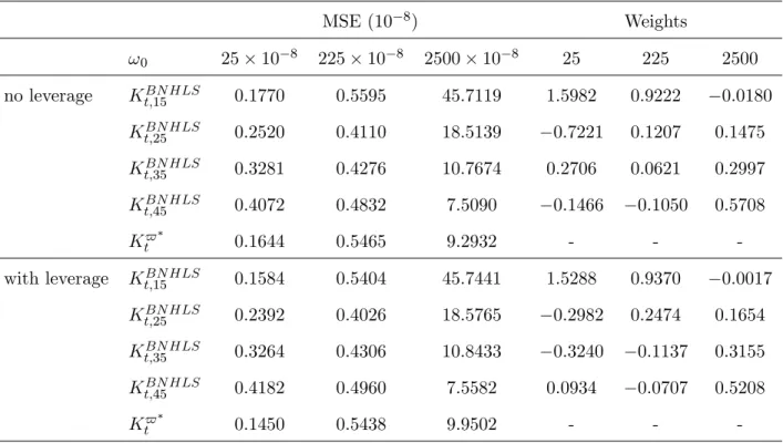
(30) Table 6. Assessing the Performance of the Adaptive Realized Kernel by Simulation under AR(1) microstructure noise and Leverage E¤ect. m = 390, T = 250, 1000 Monte Carlo replications. 8). MSE (10 !0 m. m. = 0:9. =. 0:9. 25. 10. 8. 225. 10. 8. Weights 2500. 10. 8. 25. 225. 2500. 0:0397. 0:0188. BN HLS Kt;15. 0:1697. 0:9767. 92:1028. BN HLS Kt;25. 0:2497. 0:7023. 47:4598. 0:1182. BN HLS Kt;35. 0:3355. 0:6356. 28:2403. 0:2539. BN HLS Kt;45. 0:4256. 0:6428. 18:7576. 0:0407. 0:1203. 1:2181. Kt$. 0:1589. 0:6878. 17:7389. -. -. -. BN HLS Kt;15. 0:1782. 1:8566. 204:7480. 1:5368. BN HLS Kt;25. 0:2436. 0:7142. 56:6989. 0:3094. 1:1856. BN HLS Kt;35. 0:3263. 0:5368. 25:7243. 0:3184. 0:1353. BN HLS Kt;45. 0:4169. 0:5384. 14:8193. 0:0909. Kt$. 0:1784. 0:8086. 6:9812. -. 1:3314. 1:0885 0:1691. 0:0035. 0:3174 -. 0:1082 0:3075. 0:1446 0:1024 0:1343 1:1765 -. Table 7. Assessing the Performance of the Adaptive Realized Kernel by Simulation under MA(3) microstructure noise. m = 390, T = 250, 1000 Monte Carlo replications.. MSE (10 !0 no leverage. with leverage. 25. 10. 8. 225. 10. 8) 8. Weights 2500. 10. 8. 25. 225. 1:5982. 0:9222. BN HLS Kt;15. 0:1770. 0:5595. 45:7119. BN HLS Kt;25. 0:2520. 0:4110. 18:5139. BN HLS Kt;35. 0:3281. 0:4276. 10:7674. BN HLS Kt;45. 0:4072. 0:4832. 7:5090. Kt$. 0:1644. 0:5465. 9:2932. -. -. BN HLS Kt;15. 0:1584. 0:5404. 45:7441. 1:5288. 0:9370. BN HLS Kt;25. 0:2392. 0:4026. 18:5765. 0:2982. BN HLS Kt;35. 0:3264. 0:4306. 10:8433. 0:3240. BN HLS Kt;45. 0:4182. 0:4960. 7:5582. 0:0934. Kt$. 0:1450. 0:5438. 9:9502. -. 29. 0:7221 0:2706 0:1466. 2500 0:0180. 0:1207. 0:1475. 0:0621. 0:2997. 0:1050. 0:2474. 0:5708 0:0017 0:1654. 0:1137. 0:3155. 0:0707. 0:5208. -. -.

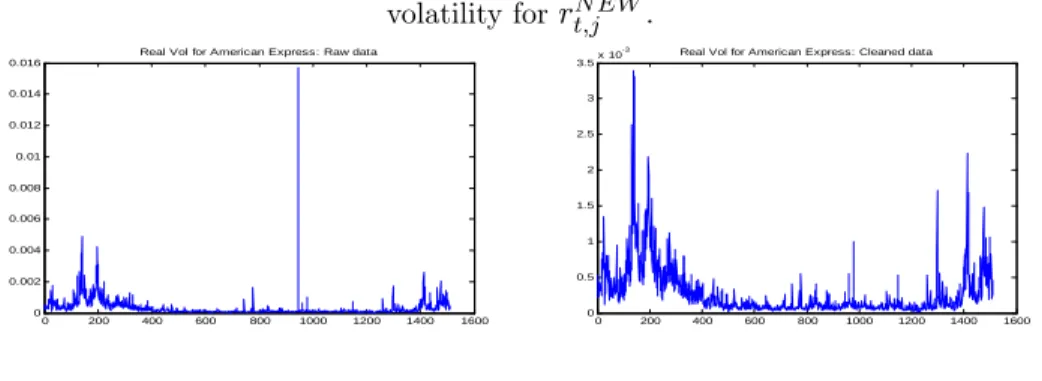
(31) Table 7 shows the simulation results for the MA(3) microstructure noise case. The upper part of the table presents the results for the scenario without leverage e¤ect while the lower part of the table presents the results for the scenario with leverage e¤ect. Qualitatively, the results are similar to what we have seen for the AR(1) noise scenario. Quantitatively, the MSEs of the IV estimators are larger than the MSE under IID noise but smaller than the MSE under AR(1) noise. This suggests that controlling for the noise variance, the more persistent the noise is, the larger the MSE of IV estimators are. This explains why larger bandwidths are needed when the dependence of the noise increases (cf. Theorem 4). In summary, our empirical investigation strategy is successful in capturing the nature of the dependence of the microstructure noise and thus, it permits to design the adaptive realized kernel in accordance with the properties of the noise.. 7. Empirical Application. For this application, we use data on twelve stocks listed in the Dow Jones Industrial (see the …rst column of Table 8). The prices are observed every one minute from January 1st , 2002 to December 31th , 2007 (1510 trading days). In a typical trading day, the market opens from 9:30 am to 4:00 pm and this results in m = 390 intradaily observations.17 There are a few missing observations (less than 5 missing data per day) which we …lled in using the previous tick method. Also, the time series of prices contain a few outlying observations that seem to be due to recording errors. To deal with such outliers in quote data, Barndor¤-Nielsen and al. (2008b) suggest to delete entries for which the spread is more that 50 times the median spread on that day. Here, we proceed similarly by applying the following cleaning rule:. N EW rt;j =. OLD if r OLD rt;j t;j OLD sign rt;j. 50. 50. rOLD ;. rOLD otherwise. OLD is the initial data and r OLD is the empirical median of r OLD across t and j. As shown where rt;j t;j. by Figure 2, this cleaning rule a¤ects very few observations and it does not remove jumps from the data.. 30.

(32) OLD . Right: realized Figure 2: Impact of the cleaning rule on the data. Left: realized volatility for rt;j N EW . volatility for rt;j -3. Real Vol for American Express: Raw data 0.016. 3.5. 0.014. Real Vol for American Express: Cleaned data. x 10. 3. 0.012. 2.5. 0.01 2 0.008 1.5 0.006 1. 0.004. 0.5. 0.002 0. 0. 200. 400. 600. 800. 1000. 1200. 1400. 0. 1600. 0. 200. 400. 600. 800. 1000. 1200. 1400. 1600. Figure 3 shows examples of volatility signature plots. Except for the General Motor index, the average RV decreases as one samples more and more sparsely. The shape of the graph for General Motors is not typical in the literature and it suggests that the bias of the RV is negative at the highest frequency.. Figure 3: Volatility signature plots for selected indices -4. 1.7. x 10. -4. Volatility signature plot for 3M Co. 2.75. x 10. -4. Volatility signature plot for American Express. 4.1. x 10. Volatility signature plot for General Motors. 2.7. 1.65. 2.65. 4.05. 1.55. Average RV. Average RV. Average RV. 1.6. 2.6. 2.55. 4. 1.5. 2.5 1.45. 1.4. 2.45. 0. 5 10 Sampling frequency in minutes. 15. 2.4. 0. 5 10 Sampling frequency in minutes. 15. 3.95. 0. 5 10 Sampling frequency in minutes. 15. Table 8 shows the output of the GMM estimation of an AR(1) noise model. Of the twelve stocks considered, the AR(1) model is not rejected for six stocks. The overidenti…cation test statistics for Intel Corp and Microsoft are only slightly above the rejection threshold. The autoregressive root m. is estimated to be positive in all cases and it is signi…cantly di¤erent from zero in cases where. the AR(1) noise model is not rejected. For the AIG stock, bm is very close to unity while it is. degenerate (i.e. equal to one) for General Motors. This suggests that the noises contaminating AIG and General Motors obey more sophisticated unit root models.. 31.

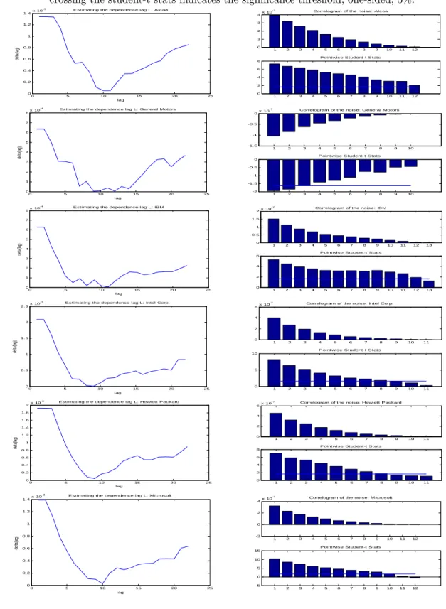
(33) Table 8: Estimating the AR(1) noise model by GMM based on 15 moments conditions At level 5%, the AR(1) model is rejected if J-stat>22.362. 3M Co.. 1:2. 10. 7. Alcoa Inc.. 1:3. 10. AIG. 3:8. American Express. ! b0. b. m. J-stat. Rejection. (2:1. 10. 8). 0:675 (0:049). 11:44. No. 6. (1:1. 10. 6). 0:931 (0:035). 31:92. Yes. 10. 4. (2:9. 10. 2). 0:998 (0:074). 9:40. No. 8:4. 10. 8. (2:1. 10. 8). 0:552 (0:110). 14:7. No. Dupont and Dupont. 3:3. 10. 7. (1:0. 10. 7). 0:846 (0:033). 20:2. No. Walt Disney. 4:4. 10. 7. (5:5. 10. 8). 0:727 (0:029). 21:8. No. General Electric. 3:8. 10. 7. (1:4. 10. 7). 0:868 (0:035). 12:2. No. General Motors. 1:7. 10. 6. (. 1:000 (. 29:2. Yes. IBM. 9:9. 10. 8. (2:1. 10. 8). 0:667 (0:065). 31:1. Yes. Intel Corp.. 4:4. 10. 7. (7:8. 10. 8). 0:766 (0:032). 22:5. Yes. Hewlett Packard. 7:9. 10. 7. (3:6. 10. 8). 0:881 (0:039). 28:3. Yes. Microsoft. 4:0. 10. 7. (7:7. 10. 8). 0:833 (0:025). 23:5. Yes. ). ). We apply the MA(L) noise model to the stocks for which the AR(1) speci…cation is rejected. e is obtained by minimizing the Table 9 shows the estimates of the dependence lag of the noise. L b is deduced from the signi…cance tests (32). (l) criterion (cf. Equation (36) and Figure 4) while L. The estimated dependence lags lies between 8 and 12 minutes.. Table 9: Estimated noise dependence lag. Figure 4 shows the plots of. Alcoa Inc (AA). e L. b L. 12. 12. General Motors (GM). 8. 3. IBM. 11. 11. Intel Corp. (INTC). 10. 9. Hewlett-Packard (HPQ). 9. 8. Microsoft (MSFT). 10. 10. (l) against L (left) and the estimated noise autocovariances (right).. To the exception of General Motors, all estimated noise correlograms are positive. This explains the 32.

(34) shape of the volatility signature plot of the General Motors index, and it supports that the estimate b. m. = 1 found previously in Table 8 is spurious. The …nal step of the empirical study concerns the estimation of the daily integrated volatility.. For all assets, we set: BN HLS BN HLS BN HLS BN HLS Kt$ = $1 Kt;15 + $2 Kt;25 + $3 Kt;35 + $4 Kt;45 ;. and minimize the variance of Kt$ with respect to $ = ($1 ; $2 ; $3 ; $4 ). We implement the adaptive realized kernel as explained in the previous section. The MSEs of all IV estimators are obtained by combining their bias and their variance (see Equations (37) and (38)). The minimum bandwidth BN HLS is unbiased under the MA(L) noises identi…ed in Table 9. H = 15 implies that Kt;H BN HLS is minimized for Table 10 shows the results. In eight cases out of twelve, the MSE of Kt;H. either H = 25 or H = 35. The MSE in increasing in H in three cases (3M Co, General Motors, IBM) and it is decreasing in one case (AIG). In the latter case for example, the initial estimators BN HLS ) have very similar variances and the di¤erences seen in their MSEs are due to the squared (Kt;H. bias term. In all other cases, the variance term dominates the squared bias term in the MSE. More often than not, the initial estimator with smallest MSE receives the largest positive weight when the noise is MA(L). As expected, the adaptive realized kernel Kt$ outperforms the most e¢ cient of the initial estimators. Arguably, the design of Kt$ can be improved by combining other estimators based on di¤erent kernel functions (Parzen, Tuckey-Hanning, Quadratic spectral). The extra cost for such an improvement resides in the derivation of the biases of the initial estimators. Figure 5 shows the estimated daily IV processes for all twelve stocks. Although many of the estimated weights in Table 10 are negative, we have found negative IV estimates for one stock only (the AIG index), and this happens for 5 days only out of 1510. An examination of the correlation matrix of the vector of the initial estimators for AIG shows that they are highly correlated. The BN HLS and K BN HLS . In fact, the noise minimum correlation is 0:9687 and it occurs between Kt;15 t;45. contaminating the AIG stock price is highly persistence (bm = 0:998), and this causes the MSE. matrix of the initial estimators to be nearly singular. For this particular stock, a bias corrected BN HLS is more reliable than K $ . version of Kt;15 t. 33.

(35) Figure 4: Estimation of MA(L) noise. Left: plot of. (l) against l. The minimum of. (l) is used as the. …rst guess of L. Right: The correlogram of the noise (top) and the associated Student-t (bottom). The line crossing the student-t stats indicates the signi…cance threshold, one-sided, 5%. -3. Estimating the dependence lag L: Alcoa. x 10. 1.4. -7. 4. Correlogram of the noise: Alcoa. x 10. 3. 1.2. 2. 1 1 0. delta(lag). 0.8. 1. 2. 3. 4. 5. 6. 7. 8. 9. 10. 11. 12. 10. 11. 12. Pointwise Student-t Stats. 0.6. 8 6. 0.4. 4. 0.2 2. 0. 0. 5. 10. 15. 20. 0. 25. 1. 2. 3. 4. 5. 6. 7. 8. 9. lag -4. 8. x 10. Estimating the dependence lag L: General Motors. -7. x 10. 0. 7. Correlogram of the noise: General Motors. -0.5. 6. -1. delta(lag). 5 -1.5. 1. 2. 3. 4. 5. 6. 7. 8. 9. 10. 9. 10. 4 Pointwise Student-t Stats 0. 3. -0.5. 2 -1. 1. -1.5. 0 0. 5. 10. 15. 20. -2. 25. 1. 2. 3. 4. 5. 6. 7. 8. lag -4. Estimating the dependence lag L: IBM. x 10. 8. -7. 2. Correlogram of the noise: IBM. x 10. 1.5. 7. 1. 6. 0.5. delta(lag). 5 0. 1. 2. 3. 4. 5. 6. 7. 8. 9. 10. 11. 12. 13. 10. 11. 12. 13. 4 Pointwise Student-t Stats 6. 3. 4. 2. 2. 1 0 0. 5. 10. 15. 20. 0. 25. 1. 2. 3. 4. 5. 6. 7. 8. 9. lag -3. x 10. 2.5. Estimating the dependence lag L: Intel Corp.. -7. 6. Correlogram of the noise: Intel Corp.. x 10. 4 2 2 1.5. delta(lag). 0. 1. 2. 3. 4. 5. 6. 7. 8. 9. 10. 11. 9. 10. 11. 9. 10. 11. 9. 10. 11. Pointwise Student-t Stats 1. 10. 0.5. 5. 0. 0. 5. 10. 15. 20. 0. 25. 1. 2. 3. 4. 5. 6. 7. 8. lag -3. x 10. 2. Estimating the dependence lag L: Hewlett Packard. -7. 6. Correlogram of the noise: Hewlett Packard. x 10. 1.8 4 1.6 2. 1.4. delta(lag). 1.2. 0. 1. 2. 3. 4. 5. 6. 7. 8. 1 Pointwise Student-t Stats 0.8. 8. 0.6. 6. 0.4. 4. 0.2 0. 2. 0. 5. 10. 15. 20. 0. 25. 1. 2. 3. 4. 5. 6. 7. 8. lag -3. 1.4. x 10. Estimating the dependence lag L: Microsoft. -7. 4. delta(lag). 1.2. Correlogram of the noise: Microsoft. x 10. 2. 1. 0. 0.8. -2. 1. 2. 3. 4. 5. 6. 7. 8. 9. 10. 11. 12. 10. 11. 12. Pointwise Student-t Stats. 0.6. 15 10. 0.4. 5. 0.2 0. 0. 0. 5. 10. 15. 20. -5. 25. lag. 34. 1. 2. 3. 4. 5. 6. 7. 8. 9.

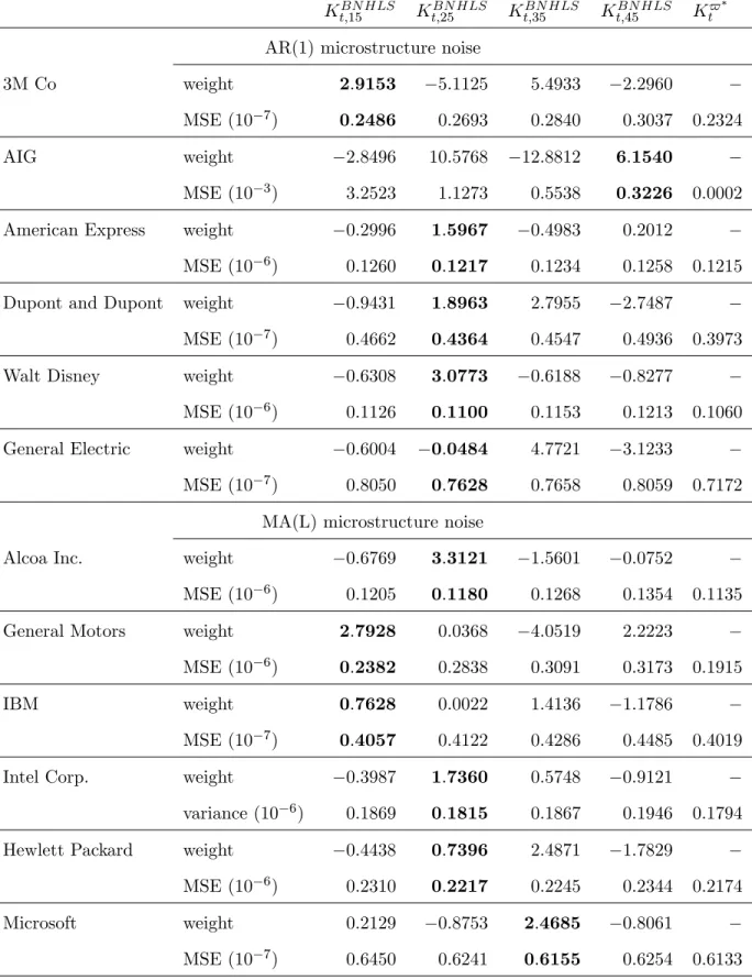
(36) Table 10: Optimal weights for the adaptive realized kernel. BN HLS Kt;15. BN HLS Kt;25. BN HLS Kt;35. BN HLS Kt;45. Kt$. AR(1) microstructure noise 3M Co. weight MSE (10. AIG. weight MSE (10. American Express. 7). weight MSE (10. General Electric. 6). weight MSE (10. Walt Disney. 3). weight MSE (10. Dupont and Dupont. 7). 6). weight MSE (10. 7). 2:9153. 5:1125. 5:4933. 2:2960. 0:2486. 0:2693. 0:2840. 0:3037. 2:8496. 10:5768. 12:8812. 6:1540. 3:2523. 1:1273. 0:5538. 0:3226. 0:2996. 1:5967. 0:4983. 0:2012. 0:1260. 0:1217. 0:1234. 0:1258. 0:9431. 1:8963. 2:7955. 2:7487. 0:4662. 0:4364. 0:4547. 0:4936. 0:6308. 3:0773. 0:6188. 0:8277. 0:1126. 0:1100. 0:1153. 0:1213. 0:6004. 0:0484. 4:7721. 3:1233. 0:8050. 0:7628. 0:7658. 0:8059. 0:2324. 0:0002. 0:1215. 0:3973. 0:1060. 0:7172. MA(L) microstructure noise Alcoa Inc.. weight MSE (10. General Motors. weight MSE (10. IBM. 6). weight MSE (10. Intel Corp.. 6). 7). weight variance (10. Hewlett Packard. weight MSE (10. Microsoft. 6). weight MSE (10. 7). 6). 0:6769. 3:3121. 1:5601. 0:0752. 0:1205. 0:1180. 0:1268. 0:1354. 2:7928. 0:0368. 4:0519. 2:2223. 0:2382. 0:2838. 0:3091. 0:3173. 0:7628. 0:0022. 1:4136. 1:1786. 0:4057. 0:4122. 0:4286. 0:4485. 0:3987. 1:7360. 0:5748. 0:9121. 0:1869. 0:1815. 0:1867. 0:1946. 0:4438. 0:7396. 2:4871. 1:7829. 0:2310. 0:2217. 0:2245. 0:2344. 0:2129. 0:8753. 2:4685. 0:8061. 0:6450. 0:6241. 0:6155. 0:6254. 35. 0:1135. 0:1915. 0:4019. 0:1794. 0:2174. 0:6133.

(37) Figure 5: Estimated daily integrated volatility by adaptive realized kernels Kt$ . -3. 3M Co.. -3. 4. Alcoa. x 10. -3. 6. 1.2. 3. 5. 1. 2.5. 4. 0.8 0.6. 2 1.5. 0.4. 1. 0.2. 0.5. 0 0. 200. 400. -3. 800 days. 1000. 1200. 1400. 0. 1600. 200. 400. 600. 800 days. 1000. 1200. 1400. -1. 1600. 4.5. 2. estimated IV. estimated IV. estimated IV. 2. 1.5. 800 days. 1000. 1200. 1400. 1600. 1000. 1200. 1400. 1600. 1000. 1200. Walt Disney. x 10. 1. 2.5 2. 1.5. 1.5. 1. 1. 0.5. 0.5. 0.5. 200. 400. 600. 800 days. 1000. 1200. 1400. 0. 1600. 200. 400. -3. General Electric. x 10. 0. 5. estimated IV. 1. 800 days. 1000. 1200. 1400. General Motors. x 10. 2. 4. 1.6. 3.5. 1.4. 3. 1.2. 2.5 2. 400. 600. -3. 800 days. 1000. 1200. 1400. 0.6 0.4. 0. 600. 800 days. IBM. x 10. 0.2. 0. 200. 400. 4. 3.5. 3.5. 3. 3. 2.5. 2.5. 600. 800 days. 1000. 1200. 1400. 0. 1600. 0. 200. 400. 600. -3. -3. Intel Corp.. x 10. 400. 1. 1. 1600. 200. 0.8. 1.5. 0.5. 200. 0. -3. 1.8. 0.5. 0. 0. 1600. 4.5 2. 1.5. 600. estimated IV. 0. -3. estimated IV. 600. 3. 2.5. 4. 400. 3.5. 3. 0. 200. -3. 4. 3.5. 2.5. 0. Dupont and Dupont. 4. 0. 2. 0. 0. x 10. 2.5. 3. 1. -3. American Express. x 10. 4.5. 600. estimated IV. 3.5. AIG. x 10. 7. 1.4. estimated IV. estimated IV. 1.6. x 10. Hewlett Packard. x 10. 3. 800 days. 1400. 1600. Microsoft. x 10. 2.5. 2 1.5 1. estimated IV. estimated IV. estimated IV. 2. 2 1.5. 1.5. 1. 1. 0.5 0.5 0. 8. 0.5. 0. 200. 400. 600. 800 days. 1000. 1200. 1400. 1600. 0. 0 0. 200. 400. 600. 800 days. 1000. 1200. 1400. 1600. 0. 200. 400. 600. 800 days. 1000. 1200. 1400. 1600. Conclusion. We design adaptive realized kernels to estimate the integrated volatility in a framework that combines, on the one hand, a Brownian stochastic volatility model with leverage e¤ect for the frictionless price, and on the other hand, a semi-parametric model for the microstructure noise. The proposed noise model is tied to the frequency at which the price data are recorded and it speci…es the noise as the sum of an endogenous term (correlated with the e¢ cient returns) and an exogenous term (uncorrelated with the e¢ cient returns). Our speci…cation for the exogenous noise nests IID, Ldependent as well as AR(1) models. The simulation results show that the adaptive realized kernels 36.

(38) achieve the optimal trade-o¤ between the discretization error and the microstructure noise. Two inference procedures are proposed for the noise parameters. The …rst procedure is based on an overidenti…ed generalized method of moments and it is designed for AR(1) types of noise. The second procedure is designed for MA(L) noises and it uses as many moment conditions as there are parameters to be estimated. The simulations show that the AR(1) inference procedure has power against MA(L) alternatives. Hence, our best investigation strategy in practice consists of …rst testing whether the noise is AR(1) and next, applying the MA(L) inference procedure if the AR(1) speci…cation is rejected. We apply this strategy to twelve stocks listed in the Dow Jones Industrial and …nd that the AR(1) noise model cannot be rejected for six stocks. For the other stocks, we apply the MA(L) noise inference procedure and …nd estimates of L that lie between 8 and 12 minutes.. Appendix: Proofs The following Lemma will be used in the proof of Theorem 1. Lemma 5 Assume that rt;j = r(1);t;j + (1 + at;j ) r(2);t;j. at;j. 1 r(2);t;j 1. + ("t;j. "t;j. 1). for some. deterministic sequence fat;j g ; j = 1; :::; m. Let ret;k be the series of non-overlapping sums of q P consecutive observations of rt;j , that is, ret;k = re(1);t;k + re(2);t;k with re(1);t;k = qk j=qk q+1 r(1);t;j and: re(2);t;k =. qk X. r(1);t;j + (1 + at;qk ) r(2);t;qk +. j=qk q+1. at;qk. q r(2);t;qk q. for k = 1; :::; mq and some positive integer q h i Pmq (m ) E RVt q = IVt +2 k=1 at;qk + a2t;qk h i (m ) V ar RVt q = O(mq ): mq X k=1. where. r(2);t;j. j=qk q+1. + ("t;qk. "t;qk. q). 1 such that mq = bm=qc. Then we have: 2 2 2 (2);t;qk +at;0 (2);t;0. Proof of Lemma 5: We have: RV (mq ) =. with:. qk X1. Pmq. 2 e(1);t;k k=1 r. +2. a2t;qmq. 2 (2);t;qmq +2mq. Pmq. e(1);t;k re(2);t;k k=1 r. 2 re(2);t;k = (1) + (2) + (3) + (4) + (5) + (6) + (7) + (8) + (9). 37. +. (! 0. Pmq. ! m;q ) ;. 2 e(2);t;k , k=1 r.

(39) (1) = (2) = (3) =. Pmq h k=1. Pmq. k=1. Pmq. i 2 2 (1 + at;qk )2 + a2t;qk r(2);t;qk + a2t;0 r(2);t;0 2 Pqk 1 r : j=qk q+1 (2);t;j. k=1 ("t;qk. (4) = 2 (5) = 2. 2 q) :. "t;qk. Pmq Pqk. 1 j=qk q+1 (1. k=1. Pmq. k=1 (1. 2 a2t;qmq r(2);t;qm : q. + at;qk ) r(2);t;j r(2);t;qk :. + at;qk ) at;qk. Pmq. q r(2);t;qk q r(2);t;qk :. "t;qk q ) r(2);t;qk : k=1 (1 + at;qk ) ("t;qk Pmq Pqk 1 (7) = 2 k=1 j=qk q+1 at;qk q r(2);t;j r(2);t;qk q : Pmq Pqk 1 (8) = 2 k=1 "t;qk q ) r(2);t;j : j=qk q+1 ("t;qk Pmq (9) = 2 k=1 at;qk q ("t;qk "t;qk q ) r(2);t;qk q : (6) = 2. Only squared terms have nonzero expectation: h. E RV. (mq ). i. =. mq X. qk X. 2 (1);t;j. +. k=1 j=qk q+1. +mq E ("t;qk = IVt + 2. qk X1. mq h i X + (1 + at;qk )2 + a2t;qk. 2 (2);t;j. k=1 j=qk q+1. h. mq X. mq X. "t;qk. q). 2. i. + a2t;0 2 (2);t;qk. at;qk + a2t;qk. 2 (2);t;qk. k=1. 2 (2);t;0. a2t;qmq. 2 (2);t;qmq. ! m;q ) + a2t;0. + 2mq (! 0. 2 (2);t;0. a2t;qmq. 2 (2);t;qmq :. k=1. where ! m;q = E ["t;j "t;j q ] is independent of t and j. Also, all the terms involved in the expression Pmq 2 re(2);t;k are uncorrelated. Thus: of k=1 V ar. " mq X k=1. where V ar((1)) = 2. V ar((2)) = 2 V ar((4)) = 4 V ar((5)) = 4 V ar((6)) = 4. 2 re(2);t;k. #. = V ar((1)) + V ar((2)) + V ar((3)) + V ar((4)) +V ar((5)) + V ar((6)) + V ar((7)) + V ar((8)) + V ar((9));. i2 Pmq h 2 2 (1 + a ) + a t;qk t;qk k=1 Pmq. k=1. 2a4t;qmq Pqk 1. l=qk q+1. Pmq Pqk k=1. Pmq. Pqk. 1 j=qk q+1 (1. k=1 (1. Pmq. 4 (2);t;qmq. 4 (2);t;qk. 4a2t;qmq 1 + at;qmq. 1 j=qk q+1. + at;qk )2. + at;qk )2 a2t;qk. 2 2 (2);t;j (2);t;l. 4 (2);t;0 2. 4 (2);t;qmq :. :. 2 2 (2);t;j (2);t;qk :. 2 2 q (2);t;qk q (2);t;qk :. + at;qk )2 V ar ("t;qk "t;qk q ) V ar r(2);t;qk P 2 2 ! m;q ) m k=1 (1 + at;qk ) (2);t;qk :. k=1 (1. = 8 (! 0. + 2a4t;0. 38.

(40) V ar((7)) = 4. Pmq Pqk k=1. 1 2 2 2 j=qk q+1 at;qk q (2);t;j (2);t;qk q :. V ar((8)) = 8 (! 0. ! m;q ). V ar((9)) = 8 (! 0. ! m;q ). Pmq Pqk k=1. 1 j=qk q+1. Pmq. 2 (2);t;j :. 2 2 k=1 at;qk q (2);t;qk q :. Hence: i hP i2 Pmq h mq 2 2 2 4 r e = 2 (1 + a ) + a V ar t;qk t;qk k=1 k=1 (2);t;k (2);t;qk Pmq Pqk 1 Pqk 1 2 2 +2 k=1 l=qk q+1 j=qk q+1 (2);t;j (2);t;l i hP Pmq Pqk 1 mq 2 2 2 2 (" " ) + 4 k=1 +V ar t;qk t;qk q j=qk q+1 (1 + at;qk ) k=1 (2);t;j (2);t;qk Pmq Pqk 1 Pmq 2 2 2 2 2 (1 + at;qk )2 a2t;qk q (2);t;qk +4 k=1 k=1 j=qk q+1 at;qk q (2);t;j (2);t;qk q (2);t;qk +4 Pmq Pqk 1 Pmq 2 2 (1 + at;qk )2 (2);t;qk + 8 (! 0 ! m;q ) k=1 +8 (! 0 ! m;q ) k=1 j=qk q+1 (2);t;j Pmq 2 2 4 4 4 at;qk q (2);t;qk +8 (! 0 ! m;q ) k=1 2a4t;qmq (2);t;qm q + 2at;0 (2);t;0 q 2. 4 4a2t;qmq 1 + at;qmq (2);t;qmq : hP mq The presence of the term V ar "t;qk k=1 ("t;qk. Pmq. 2 e(2);t;k k=1 r. 2 q). shows that V ar RV (mq ) = O(mq ). i. in the expression of the variance of. The following Lemma will be used in the proof of Theorem 3.. Lemma 6 Under the assumptions of Theorem 3, we have: i h (AC;m;1) = IVt + 2at;m + a2t;m E RVt i h (AC;m;1) = O(m): V ar RVt. 2 t;m. 2at;0 + a2t;0. 2 t;0. Proof of Lemma 6: Let rt;j = r(1);t;j +e r(2);t;j ; where re(2);t;j = (1 + at;j ) r(2);t;j at;j. ("t;j. "t;j. 1 r(2);t;j 1 +. 1 ).. We …rst note that: (AC;m;1) RVt. =. (AC;m;1) RVt. r(1) + 2. m X j=1. +2. m X j=1. (AC;m;1). where RVt r(1) = Pm 2 j=1 re(2);t;j re(2);t;j 1 . (AC;m;1). RVt. Pm. re(2);t;j r(1);t;j. 2 j=1 r(1);t;j +2. r(1);t;j re(2);t;j + 2 (AC;m;1). 1. + RVt. Pm. j=1 r(1);t;j r(2);t;j 1. m X j=1. re(2). r(1);t;j re(2);t;j. (AC;m;1). and RVt. re(2) =. 1. Pm. 2 e(2);t;j + j=1 r. re(2) = (I) + (II) + (III) + (IV ) + (V ) + (V I) + (V II) + (V III) + (IX); 39.