Positive multistate protein design

(1)

HAL Id: hal-02625007

https://hal.inrae.fr/hal-02625007

Submitted on 25 Mar 2021

HAL is a multi-disciplinary open access archive for the deposit and dissemination of sci-entific research documents, whether they are pub-lished or not. The documents may come from teaching and research institutions in France or abroad, or from public or private research centers.

L’archive ouverte pluridisciplinaire HAL, est destinée au dépôt et à la diffusion de documents scientifiques de niveau recherche, publiés ou non, émanant des établissements d’enseignement et de recherche français ou étrangers, des laboratoires publics ou privés.

Positive multistate protein design

Jelena Vucinic, David Simoncini, Manon Ruﬀini, Sophie Barbe, Thomas

Schiex

To cite this version:

Jelena Vucinic, David Simoncini, Manon Ruﬀini, Sophie Barbe, Thomas Schiex. Positive multi-state protein design. Bioinformatics, Oxford University Press (OUP), 2020, �10.1093/bioinformat-ics/btz497�. �hal-02625007�

(2)

Supplementary information

POsitive Multistate Protein design

Jelena Vucinic

1,2

, David Simoncini

1,3

, Manon Ruffini

1,2

, Sophie Barbe

1

*

and Thomas Schiex

2

*

1_{LISBP, Universit´}_{e de Toulouse, CNRS, INRA, INSA, Toulouse, France.}

2 _{MIAT, Universit´}_{e de Toulouse, INRA, Auzeville-Tolosane, France.}

(3)

1 Proof of theorem 1

This Theorem is in two parts. The first part says that positive MSD is NP-complete, the second

part says that negative MSD is NPNP-complete. We start with the first part, proving that positive

MSD is only NP-complete:

Proof. The problem is in NP because it is possible to verify a positive instance given a short

certifi-cate defined by a sequence a ∈Q

iSiand a set of conformation sequences cj = arg minc∈Q

iR j i,a[i]

Ej(a, c)

for sequence a on each of the backbone Bj ∈ B+. It suffices to compute the joint fitness of all

states and check if it is lower than the threshold k. It is complete for NP since SSD is just the case

where |B+| = 1 and is NP-complete (Pierce and Winfree,2002).

The second requires to show that the general ⊕-MSD problem is NPNP-complete.

Proof. We must prove that:

• it belongs to the class NPNP_;

• any problem in NPNP reduces to ⊕-MSD in polynomial time.

Let us introduce the following NPNP-complete problem, called ∃∀3DNF :

Given two sets of propositional variables p = (p1, . . . , pn) and q = (q1, . . . , qm), and a boolean

formula H(p, q) over these variables, in disjunctive normal form (DNF), with each cube

conjunction of three literals, is there a valuation νp of p, such that for any valuation νq of

the variables of q, νqνp(H(p, q)) is true?

Assuming we had a NP-oracle, that could solve any instance of SSD, it would be possible to verify

a positive instance of ⊕-MSD defined by a sequence a ∈ Q

iSi, by calling the oracle to compute

the minimum conformation energy Ej(a) = min_c∈Q

iC j i,a[i]

Ej(a, c) on each backbone Bj ∈ B+∪ B−

and combining these energies to check that   M Bj∈B+ min c∈Q iC j i,a[i] Ej(a, c)  −   M Bj∈B− min c∈Q iC j i,a[i] Ej(a, c)  ≤ k

Let us reduce ∃∀3DNF to ⊕-MSD . Let p = (p1, . . . , pn), q = (q1, . . . , qm), H(p, q) be a

∃∀3DNF instance, where H(p, q) = C1 ∨ · · · ∨ Ck, and for each i ∈ [|1, k|], li1, l2i and l3i are the

literals of Ci. Let us construct an instance of ⊕-MSD with n + m + k variables, represented as a

CFN:

• For each variable p ∈ p, we introduce the variable V_p with domain {T, F }, representing the

valuation of p;

• For each variable q ∈ q, we introduce the variable Vq with domain {T, F }, representing the

valuation of q;

• For each cube Ci of H(p, q), we introduce the variable VCi with domain {l

1

i, l2i, l3i}.

For each cube Ci and each variable x ∈ p ∪ q that appears in Ci, the binary cost between VCi and

Vx is defined as follows: Ex,Ci : (v, li) ∈ D Vx _{× D}V_Ci ₌    1 if v = T and li = x 1 if v = F and li = ¬x 0 otherwise

(4)

If the literal li is satisfied by the valuation v of its variable x, the corresponding binary cost is 1.

The total energy is the sum of the binary terms: E = P

x,CiEx,Ci. Given an assignment of all

variables, the energy is zero if and only if all binary terms are zero. This means that for each cube

Ci, the variable VCi is assigned a literal li that is not satisfied by the valuation νpνqdefined by the

assignment. Finally, we consider the ⊕-MSD instance with a single negative backbone:

Does there exist a ∈Q

iDVpi such that: −   min c∈Q iDVCi× Q jDVqj E(a, c)  ≤ −1

If the ∃∀3DNF instance is positive, there exists a valuation νp such that νpH(p, q) is a

tau-tology. So, if a is the assignment of the variables Vp, p ∈ p that corresponds to νp, then for any

assignment of Vq, q ∈ q, there always exists a cube Ci, which all literals are satisfied, hence, the

binary cost is greater than 1. This is equivalent to: min c∈Q iDVCi× Q jDVqj E(a, c) ≥ 1

So the ⊕-MSD instance is positive.

Conversely, if the ⊕-MSD instance is positive, there exists a ∈ Q

iDVpi, corresponding to a

valuation νp, such that the energy of any assignment of the remaining variables is greater than 1,

meaning that νpH(p, q) is a tautology.

Note that the ⊕-MSD instance consists of n + m + k variables, each with domain size less than 3, and k × (n + m) binary energies, that can be described in a 3 × 2-sized matrix, where each coefficient is straightforward to compute. Therefore, the reduction is valid and polynomial.

(5)

2 Description of protein benchmark systems

Table S 1: Description of protein systems: For each instance: system name, reference PDB id, crystallographic resolution or number of conformations for NMR structures, number of amino acid residues(N), SCOP stuctural classification(Class).

S y s te m n a m e P D B I D N u m b e r o f c o n fo rm a ti o n s N u m b e r o f re s id u e s S a c c h a ro m y c e s c e re v is ia e J -d o m a in 5 v s o 2 0 7 5 H u m a n S N F 5 /I N I1 d o m a in 5 l7 b 2 0 7 5 T ry p a n o s o m a b ru c e i P e x 1 4 N -t e rm in a l d o m a in 5 m m c 2 0 7 0 Im m u n o g lo b u lin b in d in g d o m a in o f s tr e p to c o c c a l p ro te in G 1 g b 1 6 0 5 6 C y to to x in -I f ro m t h e v e n o m o f c o b ra N . o x ia n a 5 t8 a 2 0 6 1 E 2 li p o y l d o m a in f ro m T h e rm o p la s m a a c id o p h ilu m 2 l5 t 3 3 7 7 S p id e r to x in U 4 -h e x a to x in -H i1 a 2 n 6 r 2 0 7 6 P h l P II f ro m t im o th y g ra s s p o lle n 1 b m w 3 8 9 6 A n tib a c te ri a l f a c to r-2 5 ix 5 2 0 6 8 P e p tid e t o x in S s T x f ro m S c o lo p e n d ra s u b s p in ip e s m u til a n s 5 x 0 s 2 0 5 3 R h a b d o p e p tid e N R P S D o c k in g D o m a in K j1 2 A -N D D 6 e w s 2 0 6 3 P la te le t in te g ri n -b in d in g C 4 d o m a in o f v o n W ill e b ra n d f a c to r 6 fw n 2 0 8 5 H u m a n u b iq u iti n a t 2 9 8 K 6 q f8 2 0 7 9 U b iq u iti n ( Q 4 1 N v a ri a n t) 6 jlt 2 0 7 6 S u s h i 1 d o m a in o f G A B A b R 1 a 6 h k c 2 0 7 5 S y s te m n a m e P D B I D N u m b e r o f re s id u e s H y d ro p h o b ic p ro te in f ro m S o y b e a n 1 h y p 1 .8 8 0 A lp h a -a m y la s e in h ib ito r h o e -4 6 7 A 1 h o e 2 7 4 E .c o li C o ld -s h o c k p ro te in A 1 m jc 2 6 9 B 1 im m u n o g lo b u lin -b in d in g d o m a in o f s tr e p to c o c c a l p ro te in G 1 p g a 2 .0 7 5 6 P A S F a c to r fr o m V ib ri o v u ln ifi c u s 2 b 8 i 1 .8 7 7 A p o -G o lB 4 y 2 k 1 .7 6 5 To x in is o la te d f ro m t h e M a la y a n K ra it 1 f9 4 0 .9 7 6 3 A lle rg e n p h l p 2 1 w h o 1 .9 9 6 A lp h a -s p e c tr in s rc h o m o lo g y 3 d o m a in 1 tu d 1 .7 7 6 2 H e a d p ie c e D o m a in o f C h ic k e n V ill in 1 y u 5 1 .4 6 7 R ib o s o m a l p ro te in L 3 0 f ro m t h e rm u s t h e rm o p h ilu s 1 b x y 1 .9 6 0 C -T E R M IN A L D O M A IN O F T H E R IB O S O M A L P R O T E IN L 7 /L 1 2 1 c tf 1 .7 7 4 C -M y b D N A -B in d in g D o m a in 1 g u u 1 .6 5 2 D o m a in 3 o f h u m a n a lp h a p o ly C b in d in g p ro te in 1 w v n 2 .1 8 2 T y p e I II A n tif re e z e P ro te in R D 1 f ro m a n A n ta rc tic E e l P o u t 1 u c s 0 .6 2 6 4 R (Å )

(6)

3 Solving positive min -MSD with iCFN

Recently, a guaranteed CFN-based algorithm for both positive and negative min-MSD was

intro-duced as the iCFN method (Karimi and Shen,2018). The authors did not use a reduction of the

problem to CFN but proposed and implemented a new algorithm that exploits some of the

under-lying machinery of CFN algorithms (arc consistencies (Cooper et al.,2010)). The authors showed

that their method outperforms the guaranteed COMETS software (Hallen and Donald,2016). We

therefore decided to compare Pompd against iCFN only.

The iCFN website (https://shen-lab.github.io/software/iCFN/) gives access to both the software

in binary format and to multistate design energy matrices. We wrote a first python script to translate iCFN-formatted problems into the cfn.gz CFN format that can be directly read by the CFN solver toulbar2. iCFN uses double resolution floating point energies and the cfn.gz format relies on a fixed point representation of energies. We used a “6 digits after the decimal point” representation. We wrote a second python/PyRosetta script to generate energy matrices in

iCFN-format directly from PyRosetta. These scripts make it possible to either apply Pompd _{to the}

positive min-MSD instances available on the iCFN website or to apply the iCFN algorithm on our benchmark set (for the min-MSD problem only as iCFN is not able to tackle Σ-MSD).

The iCFN command line used on the positive min-MSD problems wasiCFN -just pos -ecutDEE=2

-ecutDEE across=2 -ecutDEE seq=10 -ecut stability=5 -max conf seq=1

-max dis seq=9999 hfilesiwhich asks for one solution of the min-MSD problem, with no limitation

on the number of mutations in the produced design sequence. Except for the effect of the various pruning thresholds used by iCFN that reduce computing time, this precisely matches the min-MSD problem we solve using CFN reductions.

The iCFN multistate designs use a specific rotamer library that includes 2 extra protonated states for glutamate (Glu) and aspartate (Asp) as well as 3 protonated states for histidine (His). Because the ’cpd’ branch of toulbar2 relies on the one letter code of amino acids, it is currently unable to process the corresponding energy matrices. We therefore used the ’master’ branch of toulbar2 to solve these problems. The command line used in this case is simply -m -hbfs: which

deactivates the default Hybrid Best First Search algorithm (Allouche et al., 2015) for a simple

Depth-First Search and activates the median cost variable ordering heuristic (Allouche et al.,2014).

All computations were done on a laptop equipped with 16GB of RAM and a Intel(R) Core(TM) i7-7600U CPU at 2.80GHz.

(7)

4 Clustering distance thresholds

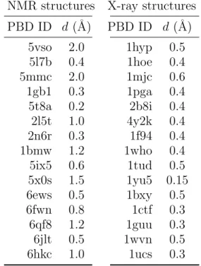
Table S 2: User-defined clustering distance thresholds (d) for each protein structure.

NMR structures X-ray structures PBD ID d (˚A) PBD ID d (˚A) 5vso 2.0 1hyp 0.5 5l7b 0.4 1hoe 0.4 5mmc 2.0 1mjc 0.6 1gb1 0.3 1pga 0.4 5t8a 0.2 2b8i 0.4 2l5t 1.0 4y2k 0.4 2n6r 0.3 1f94 0.4 1bmw 1.2 1who 0.4 5ix5 0.6 1tud 0.5 5x0s 1.5 1yu5 0.15 6ews 0.5 1bxy 0.5 6fwn 0.8 1ctf 0.3 6qf8 1.2 1guu 0.3 6jlt 0.5 1wvn 0.5 6hkc 1.0 1ucs 0.3

(8)

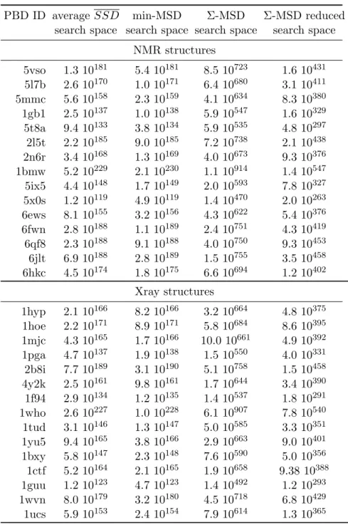
5 Search space sizes for different design problems

Table S 3: Multistate design problems: for each problem we give the average search space of four SSD problems, search space for the min-MSD problem, defined as the sum of all SSD search space sizes, the raw Σ-MSD search space size, defined by the product of the size of all variable domains and the search space size reduced by the SS constraints that impose that all states use the same sequence.

PBD ID average SSD min-MSD Σ-MSD Σ-MSD reduced

search space search space search space search space

NMR structures 5vso 1.3 10181 5.4 10181 8.5 10723 1.6 10431 5l7b 2.6 10170 1.0 10171 6.4 10680 3.1 10411 5mmc 5.6 10158 _{2.3 10}159 _{4.1 10}634 _{8.3 10}380 1gb1 2.5 10137 1.0 10138 5.9 10547 1.6 10329 5t8a 9.4 10133 3.8 10134 5.9 10535 4.8 10297 2l5t 2.2 10185 _{9.0 10}185 _{7.2 10}738 _{2.1 10}438 2n6r 3.4 10168 1.3 10169 4.0 10673 9.3 10376 1bmw 5.2 10229 2.1 10230 1.1 10914 1.4 10547 5ix5 4.4 10148 1.7 10149 2.0 10593 7.8 10327 5x0s 1.2 10119 4.9 10119 1.4 10470 2.0 10263 6ews 8.1 10155 3.2 10156 4.3 10622 5.4 10376 6fwn 2.8 10188 1.1 10189 2.4 10751 4.3 10419 6qf8 2.3 10188 9.1 10188 4.0 10750 9.3 10453 6jlt 6.9 10188 2.8 10189 1.5 10755 3.5 10458 6hkc 4.5 10174 1.8 10175 6.6 10694 1.2 10402 Xray structures 1hyp 2.1 10166 8.2 10166 3.2 10664 4.8 10375 1hoe 2.2 10171 8.9 10171 5.8 10684 8.6 10395 1mjc 4.3 10165 _{1.7 10}166 _{10.0 10}661 _{4.9 10}392 1pga 4.7 10137 1.9 10138 1.5 10550 4.0 10331 2b8i 7.7 10189 3.1 10190 5.1 10758 1.5 10458 4y2k 2.5 10161 9.8 10161 1.7 10644 3.4 10390 1f94 2.9 10134 1.2 10135 1.4 10537 1.8 10291 1who 2.6 10227 1.0 10228 6.1 10907 7.8 10540 1tud 3.1 10146 1.3 10147 5.0 10585 3.3 10351 1yu5 9.4 10165 3.8 10166 2.9 10663 9.0 10401 1bxy 5.8 10147 2.3 10148 7.6 10590 5.0 10356 1ctf 5.2 10164 2.1 10165 1.9 10658 9.38 10388 1guu 1.2 10123 4.7 10123 1.4 10492 1.2 10293 1wvn 8.0 10179 3.2 10180 4.5 10718 6.8 10429 1ucs 5.9 10153 2.4 10154 7.9 10614 1.3 10365

(9)

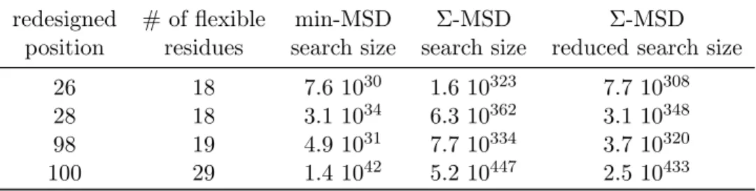
Table S 4: iCFN multistate design problems: for each problem we give the position of the redesigned residue, the number of flexible residues around the redesigned residue and the search space for the min-MSD problem, defined as the sum of all SSD search space sizes, the raw Σ-MSD search space size, defined by the product of the size of all variable’ domains and the actual search space size, reduced by the SS constraints that impose that all states use the same sequence.

redesigned # of flexible min-MSD Σ-MSD Σ-MSD

position residues search size search size reduced search size

26 18 7.6 1030 1.6 10323 7.7 10308

28 18 3.1 1034 6.3 10362 3.1 10348

98 19 4.9 1031 _{7.7 10}334 _{3.7 10}320

(10)

6 Energy difference between SSD optimal sequences and Σ-MSD

sequence

Table S 5: Difference in energy for each protein in the benchmark between the average of all SSD optimal sequences and the energy of the optimal Σ-MSD sequence (kcal).

NMR PDB Σ-MSD-SSD X-ray PDB Σ-MSD-SSD 5vso 16.0 1hyp 12.7 5l7b 10.4 1hoe 14.8 5mmc 14.3 1mjc 8.9 1gb1 11.6 1pga 12.8 5t8a 5.6 2b8i 13.3 2l5t 25.4 4y2k 5.5 2n6r 11.7 1f94 9.2 1bmw 44.9 1who 17.5 5ix5 21.7 1tud 4.2 5x0s 30.3 1yu5 6.3 Mean 19.2 Mean 10.5

(11)

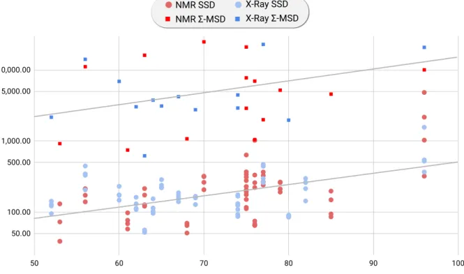
7 CPU-time for SSD and Σ-MSD as a function of protein size

NMR SSD NMR Σ-MSD

X-Ray SSD X-Ray Σ-MSD

Figure S 1: The CPU-time (Y logscale axis) is represented for SSD and Σ-MSD for both NMR and X-ray structures as a function of the protein size (X-axis). The general trend is exponential as expected with closely related slopes but a constant shift in computational cost by a factor of 1.5 orders of magnitude.q

8 3D representation of local optima networks

Figure S 2: 3D view of local optima networks. From left to right: 1bmw with min-MSD and Σ -MSD, 1who with min-MSD and Σ -MSD.

(12)

References

Allouche, D. et al. (2014). Computational protein design as an optimization problem. Artificial Intelligence, 212, 59–79.

Allouche, D. et al. (2015). Anytime hybrid best-first search with tree decomposition for weighted csp. In International Conference on Principles and Practice of Constraint Programming, pages 12–29. Springer.

Cooper, M. C. et al. (2010). Soft arc consistency revisited. Artificial Intelligence, 174(7-8), 449–478. Hallen, M. A. and Donald, B. R. (2016). Comets (constrained optimization of multistate energies by tree search): A provable and efficient protein design algorithm to optimize binding affinity and specificity with respect to sequence. Journal of Computational Biology, 23(5), 311–321. Karimi, M. and Shen, Y. (2018). iCFN: an efficient exact algorithm for multistate protein design.

Bioinformatics, 34(17), i811–i820.

Pierce, N. A. and Winfree, E. (2002). Protein design is np-hard. Protein engineering, 15(10), 779–782.