HAL Id: hal-02908680
https://hal.archives-ouvertes.fr/hal-02908680
Preprint submitted on 29 Jul 2020
HAL is a multi-disciplinary open access archive for the deposit and dissemination of sci-entific research documents, whether they are pub-lished or not. The documents may come from teaching and research institutions in France or abroad, or from public or private research centers.
L’archive ouverte pluridisciplinaire HAL, est destinée au dépôt et à la diffusion de documents scientifiques de niveau recherche, publiés ou non, émanant des établissements d’enseignement et de recherche français ou étrangers, des laboratoires publics ou privés.
An asymmetrical overshooting correction model for G20
nominal effective exchange rates
Frédérique Bec, Mélika Ben Salem
To cite this version:
Frédérique Bec, Mélika Ben Salem. An asymmetrical overshooting correction model for G20 nominal effective exchange rates. 2020. �hal-02908680�
An asymmetrical overshooting correction model for
G20 nominal effective exchange rates
Fr´ed´erique Bec
∗†M´elika Ben Salem
‡Abstract
This paper develops an asymmetrical overshooting correction autoregressive model to cap-ture excessive nominal exchange rate variation. It is based on the widely accepted perception that open economies might react differently to under-evaluation or over-evaluation of their currency because of the trade-off between fostering their net exports and maintaining their international purchasing power. Our approach departs from existing works by considering ex-plicitly both size and sign effects: the strength of the overshooting correction mechanism is indeed allowed to differ between large and small depreciations and appreciations. Evidence of overshooting correction is found in most G20 countries. Formal statistical tests confirm sign and/or size asymmetry of the overshooting correction mechanism in most countries. It turns out that the overshooting correction specification is heterogeneous among countries, even though most of Emerging Market and Developing Economies are found to adjust to over-depreciation whereas the Euro Area and the US are shown to adjust to over-appreciation only.
Keywords: nominal exchange rate, asymmetrical overshooting correction. JEL Codes: C22, F31, F41.
∗Fr´ed´erique Bec acknowledges financial support from Labex MME-DII (ANR-11-LBX-0023-01). †Thema, CY Cergy Paris Universit´e and CREST, France.
1. Introduction
Excessive exchange rate variations could be explained by the overshooting effect first identi-fied by Dornbusch (1976). In a small open economy, due to nominal price stickiness, a permanent expansionary (respectively restrictive) monetary shock would provoke a depreciation (resp. ap-preciation) of the nominal exchange rate which would go beyond the new long term exchange rate equilibrium level. Hence, this depreciation (resp. appreciation) should be followed by a few periods of appreciation (resp. depreciation) to reach the new equilibrium. Even though more so-phisticated versions of this model have been proposed, this monetary description of the exchange rate behavior has received little empirical support so far (see Rogoff 2002).
One explanation has been provided by Bjornland (2009) within the Structural Vector AutoRe-gressions framework which focuses on the estimation of the impulse response function of the exchange rate to a monetary shock. According to this author, the identification scheme of the structural shocks is misspecified as it omits the contemporaneous correlation between monetary policy and exchange rate variations. This in turn implies the so-called “delayed overshooting” put forward by Eichenbaum and Evans (1995) within this linear multivariate econometric framework. Another explanation could be that the empirical research on exchange rates has focused on nonlinear dynamics since the early 2000’s, based on the assumption that uncertainty (Kilian and Taylor 2003) or adjustment costs (Dumas 1992, Sercu, Uppal and Van Hulle 1995, Bec, Ben Salem and Carrasco 2004) could prevent investors from reacting to small deviations of the exchange rates from their fundamentals. As a consequence, the apparent success of the univariate random walk representation could stem from the omission of nonlinearities, such as the dependence of the strength of exchange rate adjustment on the size of its departures from fundamentals. As a matter of fact, empirical evidence of nonlinearity in exchange rates dynamics has been overwhelming since the 2000s as surveyed in e.g. Pavlidis, Paya and Peel (2009). Various specifications such as Threshold AutoRegressive models — see amongst others Taylor, Peel and Sarno (2001) and Sarno (2003) — or Markov Switching models — e.g. Engel and Hamilton (1990) or Cheung and Erlandsson (2005) — have been shown to outperform the linear random walk model in terms of fitting and/or forecasting. However, to our knowledge, this nonlinear framework has not been used for studying the exchange rate overshooting so far.
Besides, another branch of nonlinear models, the bounce-back models, have been found to be useful to describe transitory epochs of high growth rate GDP recovery following a recession and preceding a normal growth rate regime (see Kim, Morley and Piger 2005 for Markov Switching models or Bec, Bouabdallah and Ferrara 2014 for Threshold AutoRegressions). This mechanism is similar to an exchange rate overshooting correction after a depreciation.
The originality of our paper is to bring these strands of research together, by proposing an asymmetrical bounce-back model to investigate Dornbusch’s overshooting effect. More precisely, our goal is to shed new light on the exchange rate overshooting by allowing it to be asymmetrical across appreciation and depreciation regimes, as well as across small and large exchange rate vari-ations. To our knowledge, this has not been explored so far. The idea grounding this asymmetry is that countries could be more prompt in correcting over-appreciation than over-depreciation of their currency so as to foster their exports. On the other hand, some countries may also be concerned by over-depreciation due to the loss of purchasing power on international markets. Moreover, as stressed above, nonlinear econometric studies have shown that large exchange rates variations are
more likely to be corrected than small ones. Our main contribution is to develop an asymmet-rical overshooting correction (AOC hereafter) autoregression to capture this behavior, depending both on the sign and the size of nominal exchange rate variations. Using G20 effective nominal exchange rate data since January 1994, evidence of overshooting correction is found in most coun-tries. Formal statistical tests confirm sign and/or size asymmetry of the overshooting correction mechanism in most countries. It turns out that the overshooting correction specification is het-erogeneous among countries, even though most of Emerging Market and Developing Economies1 are found to adjust to over-depreciation whereas the Euro Area and the US are shown to adjust to over-appreciation only.
The paper is organized as follows. Section 2 introduces our original asymmetrical overshooting correction model and the method proposed to estimate it. Section 3 presents the data as well as the estimation and symmetry tests results. Section 4 concludes.
2. The asymmetrical overshooting correction autoregression
The AOC function used in the subsequent empirical investigation is inspired by the bounce-back function from Friedman’s plucking model2. This author claimed that “a large contraction in output ends to be followed on by a large business expansion; a mild contraction, by a mild expansion.” This is exactly what is expected after an exchange rate overshooting: the larger the overshooting, the larger its correction. The originality of our approach is twofold. First, we intro-duce an additional sophistication by allowing the speed of the overshooting correction to switch across small and large exchange rate variations. Second, our model also departs from Friedman’s plucking model by distinguishing positive and negative variations, whereas his model activates the rebound after a contraction only. As a result, we end up with four overshooting indicators3 associated with four different loading parameters: large depreciations (sld
t ), small depreciations
(ssdt ), small appreciations (ssat ) and large appreciations (slat ). Finally, the thresholds governing the transition between these four regimes are endogenously estimated. More precisely, we propose to represent the nominal exchange rate first difference, ∆et, by the following AOC autoregression:
∆et = λ1 m X j=0 ∆et−j−1sldt−j+ λ2 m X j=0 ∆et−j−1ssdt−j+ λ3 m X j=0 ∆et−j−1ssat−j+ λ4 m X j=0 ∆et−j−1slat−j +µ + p X k=1 ρk∆et−k + εt, ∀t = 1, · · · , T (1) with
sldt = 1 if ∆et−1≤ rdand 0 otherwise
ssdt = 1 if rd< ∆et−1≤ 0 and 0 otherwise
ssat = 1 if 0 < ∆et−1 ≤ raand 0 otherwise
slat = 1 if ∆et−1> raand 0 otherwise.
1According to the countries classification provided by the IMF in its 2019 World Economic Outlook Report. 2See Friedman (1993), who refers to his work published in the 44th NBER Annual Report in 1964.
In Equation (1), εtis a white noise with variance σ2, m ∈ N∗ governs the overshooting correction
duration, p is the autoregressive lags number. rd< 0 and ra> 0 denote two real-valued thresholds.
Note that m ≥ p in order to avoid collinearity among regressors.4
The parameters governing the strength of overshooting correction, namely the λi’s, i = 1, · · · , 4,
must be negative5 and significantly different from zero for this correction to occur, and hence to
reveal exchange rate overshooting. Let us illustrate the mechanism from the perspective of a large depreciation, i.e. the first term of Equation (1). When λ1 < 0, the term λ1Pmj=0∆et−j−1sldt−j will
increase ∆etduring m + 1 periods after a large depreciation (∆et−1≤ rd) as long as sldt−j = 1, for
j = 0, · · · , m. Consequently, m + 1 measures the duration of the overshooting correction.
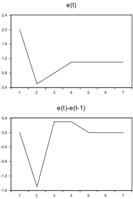
The top panel of Figure 1 plots a simulated path of the level of the nominal exchange rate after an expansionary monetary shock, for m = 1 and λ1 = −0.2. The first decrease in etbrings
the latter too low at time 2, which corresponds to the overshooting. Consequently, a bounce-back phenomenon is at work for two periods in order to reach its new equilibrium level from time 4 on: this is the overshooting correction mechanism. The bottom panel of Figure 1 plots the dynamics implied by this shock for the first difference of et, which is the dependent variable of our AOC
autoregression. There, periods 3 and 4 illustrate the role of the term λ1
Pm
j=0∆et−j−1sldt−j in
Equation (1). Note that this correction is proportional to the size of the past ∆e’s. The fourth term of Equation (1) — λ4
Pm
j=0∆et−j−1slat−j — is a function mirroring the one just described
above: after a strong appreciation, there will be evidence overshooting correction, and hence of overshooting, if λ4 < 0.
The piecewise least squares estimation method used here follows the one described in e.g. Bec, Bouabdallah and Ferrara (2014), but is extended to allow for the estimation of a second threshold. Moreover, in order to overcome possible deviations of the εt’s from a white noise sequence, the
co-variance matrix of the parameters in Equation (1) is corrected to be heteroskedasticity and autocor-relation consistent (HAC) as suggested by Newey and West (1987). The number of autoregressive lags, p, is chosen so as to eliminate serial correlation. m, rd and raare estimated simultaneously
by grid search so as to minimize the sum of squared residuals. As stressed above, m has to lie in the interval [p, ¯m]. The choice of ¯m should depend on the observation frequency of the data at hand. Here, since monthly data are used, ¯m will be set to 6 as we believe that a longer bounce-back duration would be difficult to justify by price stickiness.6 The thresholds grid intervals are denoted
[ri, ¯ri], i = d, a. rd, ¯rd, raand ¯racorrespond respectively to the 10th, 40th, 60th and 90th quantiles
of ∆et. The demeaning of ∆etensures that rdand ¯rdare negative whereas raand ¯raare positive.
This choice guarantees that at least 10% of the observations lie in each of the four regimes, so that the estimated AOC model is not driven by, say, a few important outliers.
3. Data and estimation results
Monthly data of broad effective exchange rates7 for the G20 members come from the Fed of
4For m < p, the m first ∆e
t−j−1’s under the sums becomes similar to their linear counterparts since the sum of the four indicators sx
t’s is equal to one.
5Indeed, the nominal exchange rate data used below is the number of foreign currency units per domestic currency unit, so that a decrease corresponds to a depreciation: ∆et< 0.
6As noticed in Fabiani, Loupias, Martins and Sabbatini (2007) from survey data, the full adjustment of the US consumer price index occurs within around half a year.
0.4 0.8 1.2 1.6 2.0 2.4 1 2 3 4 5 6 7 e(t) -1.6 -1.2 -0.8 -0.4 0.0 0.4 1 2 3 4 5 6 7 e(t)-e(t-1)
Figure 1: Simulated impact of λ1
Pm
j=0∆et−j−1sldt−jonetand∆etafter a depreciation at timet =
2, which triggers two periods of overshooting correction before the new exchange rate equilibrium value is reached (λ1 = −0.2 and m = 1).
St.Louis Federal Reserve Economic Data base (FRED). ∆etin Equation (1) denotes the demeaned
first difference of these effective exchange rate series. The choice of this G20 sample is motivated by the fact that this set gathers both advanced economies and Emerging Market and Developing Economies (EMDE hereafter). Table 1 reports results of the model given by Equation (1) for 17 countries.8 Indeed, results for France, Germany and Italy are not reported even though they are
members of the G20. Unsurprisingly, they follow very closely the ones obtained for the Euro area since they have adopted the Euro currency early in the sample period under consideration. Unless otherwise mentioned, the series start in January 1994 and end in December 2018.9
3.1 Overshooting correction evidence
The third column of Table 1 gives the autoregressive lags number required to remove residuals serial correlation, as confirmed by the column reporting the Q(12) Ljung-Box statistics p-value. It can be seen from the last column that some AOC models reject the null of no ARCH effect up to order 12. This should not affect our conclusions as HAC covariance matrix is used to compute the standard errors of the parameters estimates.10 Columns four to six report the estimated values
(2009), because they are computed from the exchange rates of all trade partners of a country. Hence, they are in line with the small open economy assumption underlying the overshooting effect.
8The estimate of constant term µ is not reported to save space.
9Due to unavailability or clear structural change in the exchange rate policy, data for Argentina, Brazil, Indonesia, Mexico, Russia, South Korea, and Turkey start later, as indicated in the second column of Table 1.
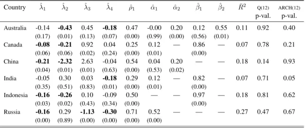
10As a matter of fact, conclusions remain unchanged using an AOC model augmented with a GARCH variance equation in these cases — see Table 4 in the Appendix.
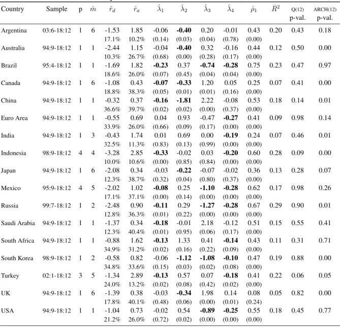
Table 1: Piecewise Least Squares estimates of the AOC model (HAC covariance matrix)
Country Sample p mˆ ˆrd ˆra λˆ1 λˆ2 ˆλ3 ˆλ4 ρˆ1 R¯2 Q(12) ARCH(12)
p-val. p-val. Argentina 03:6-18:12 1 6 -1.53 1.85 -0.06 -0.40 0.20 -0.01 0.43 0.20 0.43 0.18 17.1% 10.2% (0.14) (0.03) (0.04) (0.78) (0.00) Australia 94:9-18:12 1 1 -2.44 1.15 -0.04 -0.40 0.32 -0.16 0.44 0.12 0.50 0.00 10.3% 26.7% (0.68) (0.00) (0.28) (0.17) (0.00) Brazil 95:4-18:12 1 1 -1.69 1.82 -0.23 0.37 -0.74 -0.28 0.75 0.23 0.47 0.97 18.6% 26.0% (0.07) (0.45) (0.04) (0.04) (0.00) Canada 94:9-18:12 1 6 -1.08 0.43 -0.07 -0.33 1.20 0.05 0.25 0.07 0.41 0.00 18.8% 38.3% (0.05) (0.01) (0.01) (0.16) (0.00) China 94:9-18:12 1 1 -0.32 0.37 -0.16 -1.81 2.22 -0.08 0.53 0.18 0.14 0.01 36.6% 39.7% (0.02) (0.02) (0.00) (0.37) (0.00) Euro Area 94:9-18:12 1 1 -0.55 0.69 0.04 0.93 -0.47 -0.27 0.41 0.09 0.98 0.14 33.9% 26.0% (0.66) (0.09) (0.17) (0.00) (0.00) India 94:9-18:12 1 3 -0.43 1.74 0.01 0.69 0.00 -0.19 0.24 0.07 0.46 0.01 32.5% 11.3% (0.83) (0.13) (0.99) (0.00) (0.00) Indonesia 98:9-18:12 4 4 -3.28 2.85 -0.33 -0.02 0.03 -0.20 0.60 0.28 0.09 0.00 10.0% 10.6% (0.00) (0.85) (0.84) (0.00) (0.00) Japan 94:9-18:12 1 6 -2.08 0.34 -0.03 -0.22 -0.07 -0.02 0.36 0.13 0.28 0.07 12.3% 38.7% (0.32) (0.04) (0.80) (0.37) (0.00) Mexico 95:9-18:12 4 5 -2.02 1.02 -0.08 0.25 -1.10 -0.28 0.62 0.17 0.98 0.26 17.1% 37.1% (0.00) (0.14) (0.00) (0.00) (0.00) Russia 99:7-18:12 1 2 -2.48 0.90 -0.11 0.29 -1.27 -0.28 0.67 0.29 0.90 0.01 12.8% 36.3% (0.01) (0.22) (0.00) (0.00) (0.00) Saudi Arabia 94:9-18:12 1 1 -1.37 0.34 -0.18 -0.01 2.18 -0.12 0.51 0.15 0.55 0.41 12.3% 40.4% (0.01) (0.95) (0.06) (0.17) (0.00) South Africa 94:9-18:12 1 1 -0.88 1.62 -0.13 1.33 0.41 -0.14 0.43 0.11 0.31 0.71 34.9% 31.2% (0.02) (0.16) (0.22) (0.09) (0.00) South Korea 98:9-18:12 1 2 -0.58 0.82 -0.06 -1.12 -1.08 -0.10 0.47 0.19 0.88 0.00 34.8% 33.6% (0.15) (0.03) (0.02) (0.08) (0.00) Turkey 02:1-18:12 3 5 -1.34 2.89 -0.13 0.57 0.07 -0.18 0.41 0.22 0.06 0.05 24.0% 13.2% (0.02) (0.08) (0.42) (0.02) (0.00) UK 94:9-18:12 1 6 -1.39 0.38 -0.03 -0.34 1.98 0.14 0.08 0.05 0.82 0.00 17.8% 40.1% (0.48) (0.06) (0.00) (0.01) (0.24) USA 94:9-18:12 1 1 -1.04 0.73 -0.02 0.54 -0.89 -0.25 0.55 0.18 0.45 0.77 21.2% 26.0% (0.72) (0.02) (0.00) (0.00) (0.00)
Notes:the percentages given below ˆrdand ˆra correspond to the share of observations belonging to the large depreci-ations and apprecidepreci-ations regimes respectively. ¯R2denotes the adjusted R-squared. The column labelled ˆρ
1gives the AR(1) coefficient estimate if p = 1 and the sum of all autoregressive coefficient estimates if p > 1. Figures in bold denote significant overshooting correction coefficients at the 10%-level maximum. Student test p-values are in ( ). Q(12) (resp. ARCH(12)) p-value refers to the Ljung-Box (resp. T × R2) test of no serial correlation (resp. ARCH) up to order 12.
of m, rd and ra. In most cases, the estimated value for m is less than or equal to three. Hence,
the overshooting correction duration is rather short in general. A look at the percentages reported under the thresholds estimates in Table 1 reveals that in many countries, the upper regime contains a larger proportion of observations than the lower regime. Then, it is worth noting that in all countries, at least one of the λi’s parameters is significantly different from zero at the 10%-level,
with the correct negative sign. This provides evidence of overshooting correction which in turn points to overshooting dynamics for these exchange rates. When significant and negative, the size of the overshooting correction coefficients in the outer regimes, ˆλ1 and ˆλ4, ranges from −0.07 to
−0.33. The average of these outer regimes coefficient values implies that the monthly correction amounts to around 20% of the overshooting magnitude during m + 1 months.
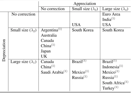
Table 2 proposes a classification of the countries by distinguishing between appreciation and depreciation, and within each regime between small and large exchange rate variations. In this Table, superscript “(1)” denotes EMDE. At first glance, the overshooting correction specification seems heterogeneous among countries. Indeed, no clear pattern appears from Table 2, but for a cluster of EMDE in the last row — which corresponds to large depreciation correction. Only Argentina and India are absent from this last row. Among EMDE, Brazil, Indonesia, Mexico, Russia, South Africa and Turkey do also correct large appreciations, as can be seen in the bottom right cell. By contrast, the Euro area and the USA correct appreciations only — see the top right cell. These countries seem to implement a “leaning-against-the-wind” foreign exchange policy in order to mitigate the initial appreciation and hence avoid large negative impacts on their current account. Finally, Canada is the only non-EMDE country which corrects large depreciations.
Table 2: Country classification according to overshooting correction parameter estimates Appreciation
No correction Small size (λ3) Large size (λ4)
Depreciation
No correction Euro Area
India(1)
USA USA
Small size (λ2) Argentina(1) South Korea South Korea
Australia Canada China(1) Japan UK
Large size (λ1) Canada Brazil(1) Brazil(1)
China(1) Indonesia(1)
Saudi Arabia(1) Mexico(1) Mexico(1)
Russia(1) Russia(1)
South Africa(1)
Turkey(1)
Notes:a country is reported in this table when the corresponding ˆλit-test p-value in Table 1 is lesser or equal to 10% and ˆλi< 0. (1) refers to EMDE.
3.2 Asymmetry of the overshooting correction
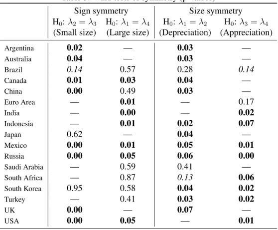
Table 3 below reports Wald tests p-values for the null hypothesis of the overshooting correction mechanism symmetry respectively depending on the sign (depreciation or appreciation) and the size (small or large) of the exchange rate variations. Overall, the results of these Wald tests support the conclusions drawn above. Wherever overshooting has been found in Table 1, a majority is significantly asymmetrical in sign and/or in size. Indeed, from the first two columns, it turns out that the sign symmetry is rejected at the 5%-level in 8 cases out of 12 for small exchange rate variations and in 7 cases out of 13 for large ones. From the last two columns, size symmetry is
Table 3: Wald tests of symmetry (p-values)
Sign symmetry Size symmetry
H0: λ2 = λ3 H0: λ1 = λ4 H0: λ1 = λ2 H0: λ3 = λ4
(Small size) (Large size) (Depreciation) (Appreciation)
Argentina 0.02 — 0.03 — Australia 0.04 — 0.03 — Brazil 0.14 0.57 0.28 0.14 Canada 0.01 0.03 0.04 — China 0.00 0.49 0.03 — Euro Area — 0.01 — 0.17 India — 0.00 — 0.02 Indonesia — 0.01 0.02 0.07 Japan 0.62 — 0.04 — Mexico 0.00 0.01 0.05 0.01 Russia 0.00 0.05 0.06 0.00 Saudi Arabia — 0.59 0.41 — South Africa — 0.87 0.13 0.06 South Korea 0.95 0.58 0.04 0.02 Turkey — 0.41 0.03 0.02 UK 0.00 — 0.07 — USA 0.00 0.05 — 0.01
Notes: figures in bold (resp. italic) denote p-values ≤ 10% (resp. ≤ 15%). No p-value is reported when no overshooting correction is found, i.e. when both λi’s are non-negative and/or non-significant.
rejected at the 5%-level in 11 cases out of 14 for depreciations and 8 out of 10 for appreciations. Actually, only two countries cannot reject sign and size symmetrical overshooting, namely Saudi Arabia and Brazil to a lesser extent. Moreover, there is no significant evidence of overshooting correction asymmetry between depreciations and appreciations in Japan, South Korea and Turkey.
4. Conclusion
Overall, our empirical results support the exchange rate overshooting feature put forward by monetary approaches of exchange rate dynamics. Indeed, most of the series considered here show evidence of overshooting correction. The asymmetry in sign and/or in size of exchange rate varia-tions revealed by our empirical results might explain the lack of overshooting evidence from pre-vious studies. Actually, the overshooting correction functional form is found to be heterogeneous among countries in such a way that cannot be embedded in a linear framework. Its theoretical modelling is on our research agenda.
References
Adolfson, M., S. Lassen, J. Linde, and M. Villani (2008) “Evaluating an estimated new keynesian small open economy model” Journal of Economic Dynamics and Control 32, 2690-2721. Bec, F., M. Ben Salem, and M. Carrasco (2004) “Test for unit-root versus threshold specification
with an application to the PPP” Journal of Business and Economic Statistics 22, 382-395. Bec, F., O. Bouabdallah, and L. Ferrara (2014) “The way out of recessions: A forecasting analysis
for some euro area countries” International Journal of Forecasting 30, 539-549.
Bjornland, H. (2009) “Monetary policy and exchange rate overshooting: Dornbusch was right after all” Journal of International Economics 79, 64-77.
Cheung, Y. and U. Erlandsson (2005) “Exchange rates and markov switching dynamics” Journal of Business and Economic Statistics23, 314-320.
Dornbusch, R. (1976) “Expectations and Exchange Rate Dynamics” Journal of Political Economy 84, 1161-1176.
Dumas, B. (1992) “Dynamic equilibrium and the real exchange rate in a spatially separated world” Review of Financial Studies5, 153-80.
Eichenbaum, M. and C. Evans (1995) “Some empirical evidence on the effects of shocks to mone-tary policy on exchange rates” Quarterly Journal of Economics 110, 975-1010.
Engel, C. and J. Hamilton (1990) ”Long swings in the dollar: Are they in the data and do markets know it?” American Economic Review 80, 689-713.
Fabiani, S., C. Loupias, F. Martins, and R. Sabbatini (2007) Pricing Decisions in the Euro Area: How Firms Set Prices and WhyOxford University Press.
Friedman, M. (1993) “The “plucking model” of business fluctuations revisited” Economic Inquiry 31, 171-177.
Kilian, L. and M. Taylor (2003) “Why is it so difficult to beat the random walk forecast of exchange rates?” Journal of International Economics 60, 85-107.
Kim, C., J. Morley, and J. Piger (2005) “Nonlinearity and the permanent effects of recessions” Journal of Applied Econometrics20, 291-309.
Newey, W. and K. West (1987) “A simple, positive semi-definite, heteroskedasticity and autocor-relation consistent covariance matrix” Econometrica 55, 703-708.
Pavlidis, E., I. Paya, and D. Peel (2009) “The econometrics of exchange rates” Handbook of Econometrics2, 1025-1083.
Rogoff, K. (2002) “Dornbusch’s overshooting model after twenty-five years: International Mone-tary Fund’s second annual research conference mundell-fleming lecture” IMF Staff Papers 49, 1-34.
Sarno, L. (2003) “Nonlinear exchange rate models: A selective overview” IMF Working Paper number 03/111.
Sercu, P., R. Uppal, and C. Van Hulle (1995) “The exchange rate in the presence of transaction costs : Implications for tests of purchasing power parity” The Journal of Finance 50, 1309-19. Taylor, M., D. Peel, and L. Sarno (2001) “Nonlinear mean-reversion in real exchange rates: Toward a solution to the purchasing power parity puzzles” International Economic Review 42, 1015-1042.
Appendix
Table 4: Maximum likelihood estimates of the AOC model (ARCH/GARCH variance)
Country λˆ1 λˆ2 λˆ3 ˆλ4 ρˆ1 αˆ1 αˆ2 βˆ1 βˆ2 R¯2 Q(12) ARCH(12) p-val. p-val. Australia -0.14 -0.43 0.45 -0.18 0.47 -0.00 0.20 0.12 0.55 0.11 0.92 0.40 (0.17) (0.01) (0.13) (0.07) (0.00) (0.99) (0.00) (0.56) (0.01) Canada -0.08 -0.21 0.92 0.04 0.25 0.12 — 0.86 — 0.07 0.78 0.21 (0.06) (0.06) (0.02) (0.24) (0.00) (0.01) (0.00) China -0.21 -2.32 2.63 -0.04 0.54 0.04 0.20 — — 0.18 0.14 0.93 (0.04) (0.01) (0.01) (0.63) (0.00) (0.53) (0.02) India -0.05 0.30 0.03 -0.18 0.29 0.12 — 0.82 — 0.07 0.71 0.05 (0.35) (0.51) (0.83) (0.01) (0.00) (0.01) (0.00) Indonesia -0.16 -0.26 0.10 -0.09 0.50 — — 0.97 — 0.18 0.81 0.62 (0.03) (0.02) (0.43) (0.34) (0.00) (0.00) Russia -0.16 0.29 -1.13 -0.30 0.71 0.52 — — — 0.27 0.47 0.67 (0.00) (0.89) (0.00) (0.00) (0.00) (0.00)
Notes:see Table 1. The ˆα’s and ˆβ’s denote the ARCH and GARCH coefficients estimates respectively: a GARCH(2,2) is used for Australia, a GARCH(1,1) for Canada, a GARCH(2,0) for China, etc. For the UK and South Korea, the GARCH augmented AOC model estimates are not reported as ARCH effects could not be eliminated.