HAL Id: hal-00316940
https://hal.archives-ouvertes.fr/hal-00316940
Submitted on 1 Jan 2002
HAL is a multi-disciplinary open access
archive for the deposit and dissemination of
sci-entific research documents, whether they are
pub-lished or not. The documents may come from
teaching and research institutions in France or
abroad, or from public or private research centers.
L’archive ouverte pluridisciplinaire HAL, est
destinée au dépôt et à la diffusion de documents
scientifiques de niveau recherche, publiés ou non,
émanant des établissements d’enseignement et de
recherche français ou étrangers, des laboratoires
publics ou privés.
structure of the background mesosphere and thermosphere using the new coupled middle atmosphere
and thermosphere (CMAT) general circulation model. Annales Geophysicae, European Geosciences
Union, 2002, 20 (2), pp.225-235. �hal-00316940�
Annales
Geophysicae
A study into the effect of the diurnal tide on the structure of the
background mesosphere and thermosphere using the new coupled
middle atmosphere and thermosphere (CMAT) general circulation
model
M. J. Harris1, N. F. Arnold2, and A. D. Aylward1
1Atmospheric Physics Laboratory, University College London, 67–73, Riding House Street, London W1P 7PP, UK 2Department of Physics and Astronomy, University of Leicester, University Road, Leicester, LE1 7RH, UK
Received: 30 November 2000 – Revised: 8 July 2007 – Accepted: 17 July 2007
Abstract. A new coupled middle atmosphere and
thermo-sphere general circulation model has been developed, and some first results are presented. An investigation into the ef-fects of the diurnal tide upon the mean composition, dynam-ics and energetdynam-ics was carried out for equinox conditions. Previous studies have shown that tides deplete mean atomic oxygen in the upper mesosphere-lower thermosphere due to an increased recombination in the tidal displaced air parcels. The model runs presented suggest that the mean residual cir-culation associated with the tidal dissipation also plays an important role. Stronger lower boundary tidal forcing was seen to increase the equatorial local diurnal maximum of atomic oxygen and the associated 0(1S) 557.7 nm green line volume emission rates. The changes in the mean background temperature structure were found to correspond to changes in the mean circulation and exothermic chemical heating.
Key words. Atmospheric composition and structure (middle
atmosphere – composition and chemistry) Meterology and atmospheric dynamics (middle atmosphere dynamics; waves and tides)
1 Introduction
There have been numerous modelling studies of tides in the Mesosphere Lower Thermosphere (MLT) region, many of which involve the comparison with observations made by in-struments on board the Upper Atmosphere Research Satellite (UARS) (e.g. Roble and Ridley, 1994; Burrage et al., 1995; Akmaev et al., 1996; Hagan et al., 1997; McLandres et al., 1997; Wu et al., 1997; Yee et al., 1997; Roble and Shepherd, 1997; Yudin et al., 1998). These have been especially useful in placing constraints on processes that influence the magni-tude of the diurnal tide in the MLT region. However, there is still uncertainty with respect to much of the physics that governs the background atmospheric structure of this region,
Correspondence to: M. J. Harris
such as collisionally induced CO215 µm radiative cooling,
exothermic chemical heating, and gravity wave dissipative heating, turbulence, and momentum drag. The situation is made more complicated by the nonlinear coupling of ener-getics, dynamics, and photochemistry.
Roble and Shepherd (1997) used the National Cen-ter for Atmospheric Research Thermosphere-Ionosphere-Mesosphere-Electrodynamics General Circulation Model (NCAR TIME-GCM, Roble and Ridley, 1994) to investigate the effects of increased lower boundary tidal forcing on pa-rameters such as meridional wind, atomic oxygen distribu-tion, and 0(1S) 557.7 nm green line volume emission rates in the MLT region. They showed that tides play an impor-tant role in atomic oxygen distribution, leading to depletions in mean atomic oxygen density at the equator, in agreement with Forbes et al. (1993) and the later study of Angelats i Col and Forbes (1998). The first mechanism put forward for this depletion was proposed by Akmaev and Shved (1980), who suggested that the net recombination increased in tidal displaced parcels of air. Angelats i Col and Forbes (1998) found that the mean vertical transport contributed to the de-pletion of O at the equator. They showed that a net downward vertical motion between 85–100 km at the equator would de-plete O through the transport to a region of increased recom-bination. It is, however, worth noting that the vertical wind fields derived in their paper showed a region of net down-welling at the equator, and updown-welling in the tropics. This differs from the derived fields for January and October pre-sented by Miyahara et al. (1991) and Fauliot et al. (1997), who showed cells of net upwelling at the equator, and down-welling in the tropics in the 80–105 km region.
In this paper, an investigation is made into the relative magnitude of the processes that are responsible for the pro-duction and loss of atomic oxygen in the mean field, and the effect of tides upon the mean temperature structure due to variations in exothermic chemical heating and mean circula-tion. This is carried out using the newly developed University College London Coupled Middle Atmosphere and Thermo-sphere (CMAT) general circulation model.
Fig. 1. Zonal mean temperature (K) (top) and zonal mean zonal wind (ms−1) (bottom) as calculated by CMAT for equinox. Positive values denote eastward winds.
2 The Coupled Middle Atmosphere and Thermosphere (CMAT) GCM
CMAT is an extension of the University College London time dependent 3-dimensional Coupled Thermosphere Iono-sphere PlasmaIono-sphere (CTIP) model (see Fuller-Rowell et al., 1996; Millward et al.,1996). It covers a vertical range from 10 mbar (∼ 30 km) to 7.587 pbar (∼ 300–600 km), numeri-cally solving the primitive nonlinear coupled equations of en-ergy, momentum, and continuity with a forward time centred space finite difference scheme. The following points high-light the main features of the model, which include updates to the original thermospheric scheme, and extensions required in order to simulate mesospheric energetics, dynamics and composition. A detailed description of CMAT is given by
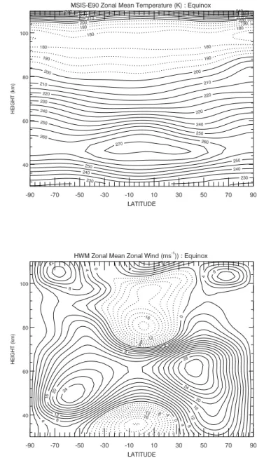
Fig. 2. Zonal mean temperature (K) as given by MSIS-E90 (top), and zonal mean zonal wind as given by HWM (ms−1) (bottom) for equinox. Positive values denote eastward winds.
Harris (2000).
(I) The model grid has a third scale height vertical, 2◦ lati-tude and an 18◦longitudinal resolution.
(II) Thermospheric heating, photodissociation and pho-toionisation are calculated due to the absorption of solar X-ray, EUV and UV radiation between 0.1– 194 nm. The fluxes, absorption and ionisation cross sec-tions between 0.1–105 nm are summarized by Fuller-Rowell (1992), and those between 105–194 nm in the Schumann-Runge continuum are given by Torr et al. (1980a), and Torr et al. (1980b). The EUV heating efficiencies are due to Roble (1987).
(III) Mesospheric heating is calculated due to the absorption of solar radiation by the ozone in the Chappuis, Hug-gins and Hartley bands, by O2in the Schumann-Runge
Bands (Strobel, 1978), and exothermic neutral chem-istry. Middle atmosphere heating efficiencies are due to Mlynczak and Solomon (1993).
(IV) The following radiative cooling parameterisations are included: 9.6 µm NO emission (Kockarts (1980)), 63 µm fine structure atomic oxygen emission (Bates (1951), Fuller-Rowell private communication (1998)), LTE and non-LTE 15.6 µm CO2 emission, with an
atomic oxygen collisional deactivation rate coefficient of 3.5 × 10⁻¹²s−1; and O39.6 µm radiative emission
(see Fomichev and Blanchet (1995)).
(V) A full mesosphere-thermosphere neutral chemical scheme is included (Allen et al., 1984; Solomon et al., 1985; Fuller-Rowell, 1992), incorporating JPL-97 reac-tion rate coefficients (DeMore et al., 1997). The effect of transport on major constituent continuity with mutual molecular diffusion is solved for O2, N2, and Ox= (O
+ O3) (see Fuller-Rowell et al., 1996). Minor species
transport is solved for N(4S), N(2D), NO, HOx= OH +
HO2+ H, H2O, H2, CO, CO2, CH4, NO2, O(1D), and
He. H2O2 and O(1D) are assumed to be in a state of
photochemical equilibrium.
(VI) High-latitude ionospheric parameters are determined from the Coupled Sheffield University High-Latitude Ionosphere Model (Quegan et al., 1982; Fuller-Rowell et al., 1996), which solves for electron and ion tem-perature; field-aligned velocities and distribution of O+
and H+; the distribution of O
2+, N2+, NO+, N+
as-suming photochemical equilibrium; and electron den-sity. High-latitude auroral precipitation, including the effect of medium energy electrons, is taken from the TIROS/NOAA auroral precipitation statistical model (Fuller-Rowell and Evans, 1987; Codrescu et al., 1997), and electric field strength from Foster et al. (1986). The effect of high-latitude, small-scale electric field variabil-ity is also included (after Codrescu et al., 2000). (VII) A Hybrid Matsuno-Lindzen parameterisation, as
out-lined by Meyer (1999), is used to calculate gravity wave drag. The source spectrum at 20 km consists of 19 waves with velocities ranging between ± 60 ms−1, propagating in both the zonal and meridional directions. The distribution of wave amplitudes is Gaussian about 0 ms−1, with the zero velocity wave having an
ampli-tude 20 times that of the ± 60 ms−1waves. The spec-trum is filtered between 20 km and the lower boundary at about 30 km, in accordance with the output from the Horizontal Wave Model (Hedin et al., 1993). The over-all intermittency factor and peak amplitude used in the parameterisation have been selected to attain a reason-able mesospheric wind structure and comparreason-able wave drag profiles, as calculated by other models. The ver-tical eddy diffusion rate coefficient is either calculated
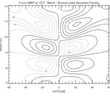
Fig. 3. Meridional winds (ms−1) as calculated by CMAT for March at 12:00 LT, with normal lower boundary diurnal tidal forcing (top), and ×2.5 lower boundary diurnal tidal forcing (bottom) southward wind contours are dotted.
in the gravity drag scheme or taken as a height depen-dent global mean based on the climatology calculated by Garcia and Solomon (1985), used in the Global Scale Wave Model (GSWM, Hagan et al., 1995)
(VIII) Lower boundary seasonal forcing is from MSIS-E90 (Hedin, 1991) and lower boundary tidal forcing from GSWM output (Hagan, private communication, 1999).
Fig. 4. Diurnal amplitude structure of meridional winds (ms−1) as calculated by CMAT for March, with normal lower boundary tidal forcing (top), and ×2.5 lower boundary tidal forcing (bottom).
3 The CMAT model runs
3.1 The standard run
The standard CMAT run presented here is for the March equinox at solar cycle minimum (F 10.7 = 76), with low ge-omagnetic activity (Kp=2+, auroral power input = 8 GW,
cross polar cap electric potential = 36 kV). The eddy diffu-sion coefficient is taken as a height dependent global mean based on the climatology calculated by Garcia and Solomon (1985) used in the GSWM, with a peak of about 75 m2/s at about 100 km. Lower boundary tidal forcing is taken from GSWM output, with a diurnal (1, 1) geopotential height am-plitude of 14 m and a phase of 20.8 h. The calculation of
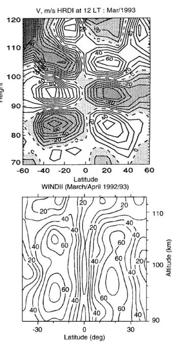
Fig. 5. Meridional winds (ms−1) at 12:00 LT for March, as mea-sured by HRDI (top) (from Yudin et al., 1997), with southward winds shaded, and the diurnal amplitude structure of meridional winds (ms−1) as measured by WINDII (bottom) (from Akmaev et al., 1997).
the atomic oxygen 557.7 nm green line emission only consid-ers the source due to recombination (Murtagh et al., 1990). CMAT was run for 30 days in a steady state.
3.2 The increased lower boundary tidal forcing run CMAT is in reasonable agreement with regards to the mor-phology of the diurnal tide in the MLT region, although it un-derestimates the amplitudes by about a factor of 2–3. Wind Imaging Doppler Images (WINDII) measured maximum am-plitudes of 60–70 ms−1 (McLandres et al., 1996), compared to about 20 ms−1as calculated by CMAT. The reason for this
Fig. 6. Meridional winds (ms−1) at 12:00 LT for March, as measured by HRDI (top) (from Yudin et al., 1997), with southward winds shaded, and the diurnal amplitude structure of meridional winds (ms−1) as measured by WINDII (bottom) (from Akmaev et al., 1997).
shortfall is due to the representation of the gravity wave dissi-pation in the model. This has also been encountered in stud-ies with the NCAR TIME-GCM (Roble and Ridley, 1995; Roble and Shepherd, 1997; Yee et al.,1997). As with the NCAR TIME-GCM, CMAT runs without gravity wave dis-sipation to produce diurnal tidal amplitudes in close agree-ment with the observations. In order to attain similar upper mesospheric amplitudes to those observed, Roble and Shep-herd (1997) increased the lower boundary tidal forcing of the NCAR TIME-GCM by a factor of 2.5. This factor is also applied in this study to the second CMAT run, such that the
peak geopotential height amplitude of the lower boundary (1, 1) diurnal tidal forcing is 35 m. All other model inputs are unchanged with respect to the standard run.
4 CMAT results and discussion
4.1 CMAT mean background atmospheric structure CMAT zonal mean temperature and zonal wind fields are shown in Fig. 1, and similar plots from the Mass
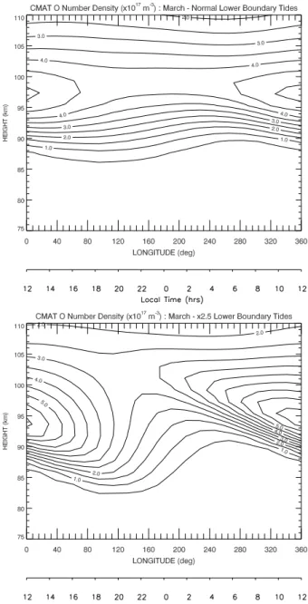
Spectrome-Fig. 7. Local time variation of atomic oxygen number density (×1017m−3) as calculated by CMAT for 12:00 LT March at the equator, with normal lower boundary tidal forcing (top), and ×2.5 lower boundary tidal forcing (bottom).
ter and ground-based Incoherent Scatter (MSIS-E90) empiri-cal model (Hedin, 1991), and the empiriempiri-cal Horizontal Wind Model (HWM) (Hedin et al., 1993), are shown in Fig. 2. The CMAT middle atmosphere temperature structure is in rea-sonable agreement with the MSIS-E90 for similar geophys-ical conditions. Both plots show a maximum stratopause temperature of about 280 K in the 45–50 km height region. The mesopause structure does, however, differ slightly in that CMAT has a local temperature maximum at about 90 km, as-sociated with exothermic chemical heating. This global fea-ture has been simulated in other modelling studies (Roble, 1995; Berger and von Zahn, 1999). Both CMAT and MSIS-E90 give mesopause minima of about 180 K at high-latitudes
Fig. 8. Diurnal mean of atomic oxygen at the equator as calcu-lated by CMAT with normal (dashed) and ×2.5 lower boundary tidal forcing (solid).
in the 100 km region.
The general morphology of the CMAT zonal mean zonal wind field is in agreement with HWM, though significant differences are present. The mid-latitude eastward zonal jets in the 55–60 km region, as calculated by CMAT, have a maximum of about 38 ms−1, compared to 28 ms−1given by HWM. Furthermore, CMAT is unable to reproduce the equa-torial and subtropical eastward winds in the 45–70 km height region. The equatorial westward wind structure between 70– 100 km is more extended in altitude in CMAT than in HWM, which shows a reversal at about 110 km. The discrepancies between CMAT and observed wind and temperature fields are most likely due to the representation of gravity wave dis-sipation in CMAT, as discussed in the previous section. 4.2 The effect of the diurnal tide
Figure 3 shows the meridional wind structure at 12:00 LT, as calculated by CMAT, for normal (top) and increased (bot-tom) lower boundary tidal forcing. With increased forcing, CMAT is in close agreement with meridional winds mea-sured by the High Resolution Doppler Imager (HRDI) on board the UARS satellite (compare Fig. 3 (bottom) to Fig. 5 (top), Yudin et al., 1997). Figure 4 gives the diurnal am-plitude structure of the meridional wind, as calculated by CMAT, for the two runs. Without increased lower bound-ary tidal forcing, CMAT gives peak amplitudes of about 20 ms−1, compared to 75 ms−1with increased forcing. The
amplitude structure determined from WINDII observations is given in Fig. 5 (bottom). The increased tidal forcing run is in reasonable agreement with the HRDI data between 80– 100 km, but it overestimates the amplitude between 100– 110 km. The diurnal amplitude and phase at 20 N with nor-mal and increased lower boundary tidal forcing are shown in Fig. 6. The phase variation with height is in reasonable agreement with WINDII measurements (e.g. Hagan et al., 1997). CMAT gives a phase of about 22 h at 96 km during
Fig. 9. Local time variation of 557.7 nm green line volume emission rate (s−1m−3) as calculated by CMAT for March at the equator, with normal lower boundary tidal forcing (top), and ×2.5 lower boundary tidal forcing (bottom).
equinox, compared to 23 h as measured by WINDII. There is little change in the CMAT simulated diurnal phase struc-ture with increased lower boundary tidal forcing. Fig-ure 9 shows O 557.7 nm green line volume emission rates, as calculated by CMAT, for both runs. With increased tidal forcing, the longitudinal morphology of the green line emis-sion is in reasonable agreement with WINDII observations (Shepherd et al., 1995). The absolute magnitudes are, how-ever, smaller in CMAT than those observed by about a fac-tor of 2, suggesting that the overall O number densities are too low. An increase in overall O of about 25% would
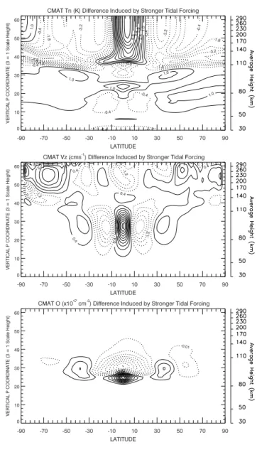
re-Fig. 10. Zonal mean difference between normal and ×2.5 lower boundary tidal forcing runs, in temperature (top), vertical wind (middle, positive values denote increase in upward winds), and atomic oxygen (bottom).
move this discrepancy. As suggested by Roble and Shepherd (1997), lower peak O densities may be in some part due to an overestimation of eddy diffusion in the model. Figure 7 shows the local time variation of atomic oxygen at the equa-tor, as calculated by CMAT, for the two runs. In agreement with the NCAR TIME-GCM simulations presented by Roble and Shepherd (1997), the atomic oxygen layer between 90– 100 km is strongly affected by tides at the equator. Oscil-lations penetrate the peak layer, resulting in much stronger diurnal variation due to changes in the overall density and vertical transport. The change in the diurnal cycle local max-imum of O density does, however, differ between CMAT and the NCAR TIME-GCM. By increasing the lower boundary tidal forcing in the NCAR TIME-GCM, Roble and Shepherd (1997) found that the local maximum of O number density at the equator, which occurs around 12:00 LT, decreased from
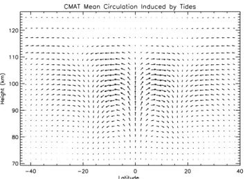
Fig. 11. Mean circulation induced with increased lower boundary tidal forcing as calculated by CMAT. The vertical winds have been scaled up by a factor of 80. Maximum vertical winds at the equa-tor in the 90–100 km height region are about 3 cm−s, and the maxi-mum meridional winds in the same height region at ± 10◦are about 7.5 ms−1.
about 6 × 10¹⁷to 5 × 10¹⁷m−3. In CMAT, the opposite oc-curs, with an increase of 5 × 10¹⁷ to 6 × 10¹⁷m−3. Since the main mechanisms responsible for the diurnal variation of O are increased with stronger tides, it follows that this can result in larger extremes of the O number density vari-ation. This would not be the case if the overall depletion of mean O was sufficiently large, for example, due to the net increase in the recombination, as discussed previously. It should be noted, however, that although Akmaev and Shved (1980) reported a decrease in O above 100 km due to tidal in-duced recombination; they showed a slight increase in peak O densities at about 95 km. This may be in some part due to the omission of mean background circulation associated with tidal dissipation in their 1-dimensional model. The peak O density in the TIME-GCM occurs at about 100 km for weak tidal forcing, which is about 3 km higher than in CMAT. This may account for the decrease rather than the increase in mean O, simulated in CMAT with increased tidal forcing. Figure 8 shows the diurnal mean atomic oxygen vertical profile at the equator for both CMAT runs. The mean peak in O is seen to decrease by about 11%, and the integrated column between 80–140 km by about 4%. Between about 80–90 km, stronger tidal forcing increases O number densities, as expected with tidal oscillations of the O peak layer that penetrate to lower altitudes.
Figure 10 shows the difference fields for zonal mean tem-perature (top), zonal mean vertical wind (middle), and zonal mean atomic oxygen (bottom), caused by stronger lower boundary tidal forcing. The trends in atomic oxygen and temperature between ±20◦in latitude are in agreement with the modelling study of Forbes and Roble (1993), and the cell-like vertical wind structure induced by increased dissi-pating tides is similar to mean vertical wind fields derived from WINDII observations (Fauliot et al., 1997). Figure 11
contributions of the terms in the Ox production/loss
equa-tion, and can give little information as to the components in each term. For example, the net loss associated with verti-cal advection may have two components. It could be due to a combination of net upward vertical motion of O poor air, and the increased recombination effect associated with tidal oscillations.
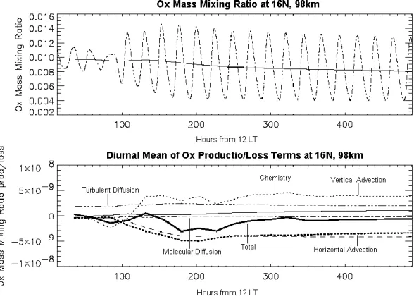
Figure 12 (top) shows the Oxmass mixing ratio at 98 km
16◦N for a CMAT run when increased lower boundary forc-ing is introduced. It takes 2–3 days for the effect of increased tides to fully propagate to this altitude, after which the ampli-tude in the oscillations of Oxis seen to increase. A decrease
in the mass mixing ratio is observed, as seen in the diurnal mean Ox number density trend. Figure 12 (bottom) shows
the diurnal mean production and loss terms of Oxmass
mix-ing ratio for the same location and run. As the tides become stronger at this altitude, diurnal loss due to horizontal advec-tion increases. The contribuadvec-tion from diurnal mean vertical advection is positive due to net downward motion, though it seems to lag behind the loss due to horizontal advection. This would be consistent with increased chemical loss in verti-cally displaced parcels of air as the increased tides first prop-agate into this region. As the concentration of O falls, this effect would decrease, and the positive contribution of ver-tical advection would catch up with the negative horizontal terms. The chemical and meridional advection production-loss terms slowly increase, acting to slow the rate of production-loss of Ox. With respect to chemistry, this is consistent with the
lower Ox concentrations, leading to decreased
recombina-tion. This results in an overall increase in chemical produc-tion, since the solar dissociation production of O is largely unaffected by increased tides. The slow increase in merid-ional advection is consistent with falling concentrations at the equator. This acts to reduce the latitudinal gradient Ox,
which, in turn, decreases the magnitude of the loss due to net outward flow from the equator.
The change in the mean temperature with increased tidal forcing was shown in Fig. 10 (top). Although the changes are small, it is interesting to note the processes responsible, since they highlight the complexity of the coupling mechanisms in the MLT region. Analysis of the production and loss terms in the CMAT energy equation show that the decrease in temper-ature between 90–110 km and the increase below 90 km are
Fig. 12. (top): Oxmass mixing ratio at 16◦N, 98 km, (dotted line), and diurnal mean of Oxmass mixing ratio (solid line) as calculated by
CMAT when introducing tides; (bottom) Diurnally averaged production and loss terms of Oxat the equator for the same run and location.
in some part due to changes in exothermic chemical heating. This process is the major energy source in the MLT region, as calculated by CMAT (see Fig. 13). The global mean val-ues shown are in reasonable agreement with previous studies (Mlynczak and Solomon, 1993; Reis et al., 1994; Ward and Fomichev, 1993; Zhu et al., 1999). Increased tides deplete O in the 90–110 km region, and increase it below 90 km. This leads to a decrease in chemical heating between 90–100 km and an increase below 90 km, with corresponding changes in temperature. Similar runs with chemical heating deactivated above 75 km show similar temperature variations due to in-creased tides, but with a smaller magnitude. The remain-ing variations with chemical heatremain-ing deactivated are due to changes in advection. Similar to the changes in mean O, be-low 90 km, the increase in temperature is due to an increase in the positive contribution of the vertical advection term, whereas between 90–110 km, there is an increased cooling due to horizontal advection.
5 Conclusions
Similar runs to those carried out by Roble and Shepherd (1997) have been made with a new mesosphere and thermo-sphere general circulation model. CMAT was able to simu-late many diurnal tidal features observed in the MLT region. The runs suggest that tides act to reduce the peak in mean O density at the equator, but not sufficiently so that the
diur-Fig. 13. The main CMAT global mean heating and cooling rates in the MLT region in Kday−1with normal lower boundary tidal forc-ing. TSOL+O(1D)is the total of heating due to the absorption of
so-lar radiation and the quenching of O(1D); Tchemis total exothermic
chemical heating; H+O3is heating due to the reaction of
hydro-gen and ozone (with a heating efficiency of 0.6); Oxis heating due
to oxygen recombination reactions; CO2is cooling due to 15 µm
emission from CO2; Ktis cooling due to turbulent heat conduction.
nal cycle local maximum decreases with increased tidal forc-ing. The diurnal cycle local maximum values of green line
ture, are most likely due to the representation of gravity wave drag in the model. This will be addressed with the update to a more sophisticated parameterisation, such as that of Hines (1997a, b).
Acknowledgement. The authors wish to thank I. C. F. Mueller-Wodarg for his helpful discussion, and the two referees for their helpful comments. The research is supported by grants from PPARC. The work was carried out on the Miracle supercomputer, at the UCL Hyperspace computing centre, which is funded by U. K. Particle Physics and Astronomy Research Council.
The Editor in Chief thanks R. A. Akmaev and another referee for their help in evaluating this paper.
References
Akmaev, R. A. and Shved, G. M.: Modelling of the composition of the lower thermosphere taking account of the dynamics with ap-plication to tidal variations of the [OI] 5577 ˚Aairglow, J. Atmos. Terr. Phys., 42, 705–716, 1980.
Akmaev, R. A., Yudin, V. A., and Ortland, D. A.: SMLTM simu-lations of the diurnal tide: comparison with UARS observations, Ann. Geophysicae, 15, 1187–1197, 1997.
Akmaev, R. A.: Simulation of tides with a spectral meso-sphere/thermosphere model, Geophys. Res. Lett., 23, 2173, 1996.
Allen M., Lunine, J. I., and Lang, Y. L.: The vertical distribution of ozone in the mesosphere and lower thermosphere, J. Geophys. Res., 89, 4841, 1984.
Angelats i Col, M. and Forbes, J. M.: Dynamical influences on atomic oxygen and 5577 ˚Aemission rates in the lower thermo-sphere, Geophys. Res. Letts., 25, 4, 461–464, 1998.
Bates, D. R.: The temperature of the upper atmosphere, Proc. Phys. Soc., London, 64B, 805, 1951.
Berger, U. and von Zahn, U.: The two-level structure of the mesopause: A model study, J. Geophys. Res., 104, 22 083– 22 093, 1999.
Burrage, M. D., Hagan, M. E., Skinner, W. R., Wu, D. L., and Hays, P. B.: Long-term variability in the solar diurnal tide observed by HRDI and simulated by the GSWM, Geophys. Res. Lett., 22, 2641, 1995.
Codrescu, M. V., Fuller-Rowell, T. J., Roble, R. G., and Evans, D. S.: Medium energy particle precipitation influences on the mesosphere and lower thermosphere, J. Geophys. Res., 102, A9, 19 997, 1997.
Fomichev, V. I., Blanchet, J.P., and Turner, D. S.: Matrix param-eterization of the 15 µm band cooling in the middle and upper atmosphere for variable CO2 concentration, J. Geophys. Res., 103, D10, 11 505–11 528, 1998.
Forbes, J. M. and Roble, R. G.: Acceleration, heating, and compo-sitional mixing of the thermosphere due to upward propogating tides, J. Geophys. Res., 98, A1, 311–321, 1993.
Foster, J. C., Holt, J. M., Musgrove, R. G., and Evans, D. S.: Iono-spheric convection associated with discrete levels of particle pre-cipitation, Geophys. Res. Lett., 13, 656, 1986.
Fuller-Rowell, T. J. and Rees, D.: A three-dimensional time-dependant global model of the thermosphere, J. Atmos. Sci, 37, 2545, 1980.
Fuller-Rowell, T. J. and Evans, D. S.: Height-integrated Pedersen and Hall conductivity patterns inferred from the TIROS-NOAA satellite data, J. Geophys. Res., 92, 7606, 1987.
Fuller-Rowell, T. J.: Modelling the solar cycle change in nitric ox-ide in the thermosphere and upper mesosphere, J. Geophys. Res., 98, 1571, 1992.
Fuller-Rowell, T. J., Rees, D., Quegan, S., Moffett, R. J., Codrescu, M. V., and Millward, G. H.: A coupled thermosphere ionosphere model, Solar terrestrial energy program (STEP), handbook of ionospheric models, (Ed) Schunk, R. W., 1996.
Garcia, R. R. and Solomon, S.: A numerical model of the zonally averaged dynamical and chemical structure of the middle atmo-sphere, J. Geophys. Res., 90, 3850–3868, 1985.
Hagan, M. E., Forbes, J. M., and Vial, F.: On modelling migrating solar tides, Geophys.Res.Lett., 22, 893–896, 1995.
Hagan, M. E., McLandres, C., and Forbes, J. M.: Diurnal tidal vari-ability in the upper mesosphere and lower thermosphere, Ann. Geophysicae, 15, 1176–1186, 1997.
Harris, M. J.: A new coupled terrestrial mesosphere-thermosphere general circulation model: Studies of dynamic, energetic, and photochemical coupling in the middle and upper atmosphere, PhD Thesis, University of London, UK, submitted, 2000. Hedin, A. E.: Extension of the MSIS Thermosphere model into the
middle and lower atmosphere, J. Geophys. Res., 96, A2, 1159, 1991.
Hedin, A. E., Flemming, E. L., Manson, A. H., Schmidlin, F. J., Av-ery, S. K., and Franke, S. J.: Empirical wind model for the mid-dle and lower atmosphere 1: Local time average, NASA Tech. Memo. NASA TM-104 581, 1993.
Hines, C. O.: Doppler Spread parameterisation of gravity wave mo-mentum deposition in the middle atmosphere, Part I, Basic for-mulation, J. Atmos. Solar-Terr. Phys., 59, 371–386, 1997a. Hines, C. O.: Doppler Spread parameterisation of gravity wave
mo-mentum deposition in the middle atmosphere, Part II, Broad and quasi monochromatic spectra, and implementation, J. Atmos. Solar-Terr. Phys., 59, 387–400, 1997b.
Kockarts, G.: Nitric oxide cooling in the terrestrial thermosphere, Geophys. Res. Lett., 7, 2, 137, 1980.
McLandres, C., Shepherd G. G., and Solheim B. H.: Satellite ob-servations of thermospheric tides : Results from the wind imag-ing interferometer on UARS, J. Geophys. Res., 101, 4093–4114, 1996.
McLandres, C.: Seasonal variability of the diurnal tide: Results from the Canadian middle atmosphere general circulation model, J. Geophys. Res., 102, D9, 29 747, 1997.
Meyer, C.: Gravity wave interactions with mesospheric planetary waves: A mechanism for penetration into the thermosphere-ionosphere system, J. Geophys. Res., 104, 28 181–28 196, 1999. Millward, G., Moffett, R. J., Quegan, S., and Fuller-Rowell, T. J.: A Coupled Thermosphere-Ionosphere-Plasmasphere Model (CTIP), Solar Terrestrial Energy Program (STEP) Handbook, (Ed) Schunk, R. W., 1996.
Miyahara, S., Portnyagin, Yu. I., Forbes, J. M., and Solovjeva, T. V.: Mean zonal acceleration and heating of the 70–110 km region, J. Geophys. Res., 96, 1225–1238, 1991.
Mlynczak, M. G. and Solomon, S.: Middle atmosphere heating by exothermic chemical reactions involving odd hydrogen species, Geophys. Res. Lett., 18, 37–40, 1991.
Mlynczak, M. G. and Solomon, S.: A detailed study of heating ef-ficiency in the middle atmosphere, J. Geophys. Res., 98, 10 517– 10 541, 1993.
Murtagh, D. P., Witt, G., Stegman, J., McCade, I. C., Llewellyn, E. J., Harris, F., and Greer, R. G. H.: An assessment of proposed O(1S) and O2(b16+b) nightglow excitation parameters, Planet. Space. Sci., 38, 43, 1990.
Quegan, S., Bailey, G. J., Moffett, R. J., Heelis, R. A., Fuller-Rowell, T. J., Rees, D., and Spiro, A. W.: A theoretical study of the distribution of ionisation in the high-latitude ionosphere and the plasmasphere: First results of the mid-latitude trough and the light ion trough, J. Atm. Terr. Phys., 44, 619, 1982.
Reis, M., Offerman, D., and Brasseur, G.: Energy released by re-combination of atomic oxygen and related species at mesopause heights, J. Geophys. Res., 99, D7, 14 585, 1994.
Roble, R. G., Ridley E. C., and Dickenson, R. E.: On the global mean structure of the thermosphere, J. Geophys. Res., 92, A8, 8745–8758, 1987.
Roble, R. G. and Ridley, E. C.: A thermospheric-ionosphere-mesosphere-electrodynamics general circulation model (time-GCM): Equinox solar cycle minimum simulations (30–500 km), Geophys. Res. Letts., 21, 6, 417, 1994.
Roble, R.: Energetics of the mesosphere and thermosphere, Upper mesosphere and lower thermosphere: A review of experiment and theory, Geophysical monograph 87, AGU, 1995.
Roble, R. G. and Shepherd, G. G.: An analysis of wind imaging interferometer observations of O(1S) equatorial emission rates using the thermosphere-ionosphere-mesosphere electrodynam-ics general circulation model, J. Geophys. Res., 102, A2, 2467, 1997.
Shepherd, G. G., McLandres, C., and Solheim, B. H.: Tidal in-fluence on O(1S) airglow emission rate distributions at the ge-ographic equator as observed by WINDII, Geophys. Res. Lett., 22, 275, 1995.
Solomon, S., Garcia, R. R., Olivero, J. J., Bevilacqua, R. M., Schartz, P. R., Clancy, R. T., and Muhleman, D. O.: Photochem-istry and transport of carbon monoxide in the middle atmosphere, J. Atmos. Sci., 42, 1072, 1985.
Strobel, D. F.: Parameterization of the atmospheric heating rate from 15 to 120 km due to O2and O3absorption of solar
radi-ation, J. Geophys. Res., 83, 6225, 1978.
Torr, M. R., Richards, P. G., and Torr, D. G.: A new determination of ultraviolet heating efficiency in the thermosphere, J. Geophys. Res., 85, 6819, 1980a.
Torr, M. R., Richards, P. G., and Torr, D. G.: The solar ultravio-let heating efficiency in the mid-latitude thermosphere, Geophys. Res. Lett., 6, 673, 1980b.
Ward, W. E. and Fomichev, V. I.: On the role of atomic oxygen on the dynamics and energy budget of the mesosphere and lower thermosphere, Geophys. Res. Lett, 12, 1199, 1993.
Wu, D. L., Hays, P. B., and Roble, R. G.: Doppler imager wind measurements with simulations from the NCAR thermosphere-ionosphere-mesosphere-electrodynamics circulation model, 101, D14, 19 147, 1997.
Yee, J.-H., Crowley, G., Roble, R. G., Skinner, W. R., Burrage, M. D., and Hays, P. B.: Global simulations and observations of O(1S), O2(16)and OH mesospheric nightglow emissions, 102, A9, 19 949, 1997.
Yudin, V. A., Khattatov, B. V., Geller, M. A., Ortland, D. A., McLandres, C., and Shepherd, G. G.: Thermal tides and studies to tune the mechanistic tidal model using UARS observations, Ann. Geophysicae, 15, 1205–1220, 1997.
Yudin, V. A., Geller, M. A., Khattatov, B. V., Ortland, D. A., Bur-rage, M. D., McLandres, C., and Shepherd, G. G.: TMTM simu-lations of tides: Comparison with UARS observations, Geophys. Res. Lett., 25, 2, 221, 1998.
Zhu, X.: Numerical modeling of Chemical-Dynamical Coupling in the Upper Stratosphere and Mesosphere, J. Geophys. Res., 104, D19, 23 995, 1999.