A Dynamic Multiscale Viscosity Algorithm for
Shock Capturing in Runge Kutta Discontinuous
Galerkin Methods
by
Jean-Baptiste Brachet
Submitted to the Department of Aeronautics and Astronautics
in partial fulfillment of the requirements for the degree of
Master of Science in Aerospace Engineering
at the
MASSACHUSETTS INSTITUTE OF TECHNOLOGX
May 2005
[Taj@
Massachusetts Institute of Technology 2005.
Author ...
Department of Aeronautics and Astronautics
J~ff= _,2005
Certified by...
...
.A
...
. . . . . . . .Jaime Peraire
Professor of Aeronautics and Astronautics
The
rvisor
...
6 ...
Jaime Peraire
Chairman, Department Committee on Graduate Students
-I
MASSACHUSETTS INSTMITE OFTECHNOLOGY
JUN 2 3 2005
LIBRARIES
All rights reserved.
I
Accepted by ...
A Dynamic Multiscale Viscosity Algorithm for Shock
Capturing in Runge Kutta Discontinuous Galerkin Methods
by
Jean-Baptiste Brachet
Submitted to the Department of Aeronautics and Astronautics on May 20, 2005, in partial fulfillment of the
requirements for the degree of Master of Science in Aerospace Engineering
Abstract
In order to improve the performance of higher-order Discontinuous Galerkin finite element solvers, a shock capturing procedure has been developed for hyperbolic equa-tions. The Dynamic Multiscale Viscosity method, originally presented by Oberai and Wanderer [8, 9] in a Fourier Galerkin context, is adapted to the Discontinuous Galerkin discretization. The notions of diffusive model term, artificial viscosities, and the Germano identity are introduced. A general technique for the evaluation of the multiscale model term's parameters is then presented. This technique is used to perform efficient shock capturing on an one-dimensional stationary Burgers' equation with 1-parameter and 2-parameter model terms. Corresponding numerical results are shown.
Thesis Supervisor: Jaime Peraire
Acknowledgments
I would like to express my gratitude to the many people who supported me during these two years at MIT.
First of all, I would like to thank all the ACDL staff: my advisor, Professor Peraire, for his help and availability during this research; the Project X team, especially Professor Darmofal and Bob Haimes, for having shared their insights with me; and Jean for her support and patience.
My stay at MIT would not have been such a wonderful experience without the numerous friends I met here. I therefore would like to thank my friends from the lab: Garrett, Krzysztof, Todd, Mike, Dan and Sudeep. Thanks you for your cheerfulness ! Thanks also to the french colonies at ICAT and GTL, to Jeff, Rick, Emmanuel, Theo, to the Thomas and to Pierre, who didn't unfortunately swim across the Charles as promised. Thanks to Jorge for having helped me to practice my English as well as my French and German accents.
Finally, I would like to thank my wife, Pascale, for her love and support during these two years.
Contents
1 Introduction
2 Time and space discretizations
2.1 Mathematical formulations . . . . 2.1.1 Purely convective equations . . . . 2.1.2 Convection-diffusion equations . . . . 2.1.3 Burgers' equations . . . . 2.1.4 Weak formulations . . . . 2.2 Discontinuous Galerkin method . . . . 2.2.1 Application to purely convective problems . 2.2.2 Application to convection-diffusion problems 2.2.3 One-dimensional implementations . . . . 2.3 Runge-Kutta schemes . . . .
3 Dynamic Multiscale Viscosity
3.1 Motivation and notation . . . . 3.1.1 Existing shock-capturing techniques . . . . . 3.1.2 Advantages of dMSV schemes . . . . 3.1.3 M odel term . . . .. . . . 3.2 Description of the dMSV methodology . . . . 3.2.1 The variational Germano identity . . . . 3.2.2 Evaluation of the model parameters . . . . . 3.3 Discontinuous Galerking implementation . . . .
13 15 . . . . 15 . . . . 15 . . . . 16 . . . . 16 . . . . 16 . . . . 17 . . . . 18 . . . . 2 1 . . . . 22 . . . . 24 27 . . . . 28 . . . . 28 . . . . 28 . . . . 29 . . . . 29 . . . . 30 . . . . 33 . . . . 35
3.3.1 Challenges for a DG implementation . . . . 35
3.3.2 1-viscosity and 2-viscosity model terms . . . . 38
3.3.3 Projections . . . . 43
3.3.4 Algorithms structure . . . . 45
4 Results 47 4.1 1-viscosity model term . . . . 47
4.1.1 Smooth solution. . . . . 47
4.1.2 Burgers' equation . . . . 49
4.2 2-viscosity model term . . . . 52
4.2.1 smooth solution . . . . 53
4.2.2 Burgers' equation . . . . 54
4.3 C onclusion . . . . 60
A 1-viscosity model term consistency condition 63
List of Figures
3-1 Projections of the step function on (Li)i=o,...,25 . . . . 38 3-2 domains affected by the artificial viscosity 9 at scales 5 (right) and 3
(left) . . . . 4 0 3-3 domains affected by the artificial viscosities T and = at scales 5 (right),
3 (m iddle), and 1 (left) . . . . 42 3-4 dMSV algorithms structure . . . . 45
4-1 1-viscosity dMSV - convergence rate for a smooth solution . . . . 49 4-2 iterated solution (top) and artificial viscosity evolution (bottom) over
the time period [0, -]for Pe=100 . . . . 50 4-3 iterated solution (top) and artificial viscosity evolution over the time
period
[L,
4] (bottom) for Pe=+inf. . . .
514-4 2-viscosity dMSV - convergence rate for a smooth solution . . . . 54 4-5 iterated solution (top) and artificial viscosities evolution over the time
period [0, -] (bottom) for Pe=5 . . . . 55 4-6 iterated solution (top) and artificial viscosities evolution over the time
period [0, -] (bottom) for Pe=10 . . . . 56 4-7 iterated solution (top) and artificial viscosities evolution over the time
period [0, -] (bottom) for Pe=100 . . . . 57 4-8 iterated solution (top) and artificial viscosities evolution over the time
period
[0,
7] (bottom) for Pe= 106. . . .
584-9 iterated solution (top) and artificial viscosities evolution over the time period [0, -] (bottom) for Pe=+ inf . . . . 59
List of Tables
4.1 L2 error for the transport equation with a smooth initial condition and a 1-viscosity model term . . . . 48 4.2 L2 error for the transport equation with a smooth initial condition and
Chapter 1
Introduction
Since their introduction during the 1970s, Computational Fluid Dynamics tools have become increasingly used in the industry, resulting in enhanced designs, shorter de-velopment costs and increased safety levels. This success calls for CFD tools that are both faster and more accurate, as they are expected to deal with more and more complex problems. Although grid refinement related techniques are a possible mean to increase the accuracy of CFD codes, they do not seem to provide a satisfactory solution for many applications when used on their own. Compared to them, higher-order methods, presented by Cockburn and Shu (see for example
[1]),
seem much more attractive and could ultimately change the current paradigm in CFD by intro-ducing new codes that would combine high accuracy and reliability in a cost efficient manner.However, many challenges still need to be addressed before a CFD code taking full advantage of high-order methods can be put into operations. These challenges are various and range from generating high-order grids to the visual presentation of information. Many of these challenges are of course related to solving techniques and, among those, obtaining efficient shock capturing capabilities is one of the most critical. .
One possible approach to shock capturing is to introduce artificial viscosity in the equation. Provided the correct amount of viscosity is put into the system, the shock can be properly and accurately solved. Recently, Assad Oberai and John Wanderer
have presented a promising method for computing this artificial viscosity from the system itself [9]. This method, called the Dynamic Multiscale Viscosity Method, is based on a variational formulation of the Germano identity, which is widely used in the Large Eddy Simulation of turbulent flows, and has been implemented and tested in a spectral context, using Fourier Galerkin discretizations.
The purpose of this thesis is to investigate the potential of this Dynamic Multi-scale Viscosity Method (dMSV) in a Discontinuous Galerkin (DG) context. Although a number of finite differences or finite elements methods can achieve high order ac-curacy, the finite element Discontinuous Galerkin method has several advantages. In this method, the coupling between elements is achieved through numerical fluxes evaluated at the boundaries of each element, making the implementation of boundary conditions a straightforward task, whereas other higher-order schemes often require large stencils that complicate the implementation of these conditions. Additional ben-efits are obtained through the use of DG, such as an easy implementation of parallel computing techniques.
Although several methods for capturing shocks, such as Weighted Essentially Non-Oscillatory (WENO) schemes [12], have been developped, none of them has yet set a standard. Many of these methods are based on the detection of shocks and on the reconstruction of lower-order, oscillations-free, solutions on the corresponding cells. The design of an efficient and reliable shock detection algorithm is often a challenge. Similarly, the reconstruction of the solution over the troubled cells requires the use of a stencil, which may lead to difficult implementations of some kinds of boundary conditions. As we shall see it later, the dMSV approach has neither of these issues: it does not require any shock detection nor does it need any reconstruction for the solution.
In this context, a dMSV-based shock-capturing algorithm for stationary shocks has been developped. This algorithm has been tested with two different model terms on a fifth-order solution, the stationary shock being generated by Burgers' equation. The results of these tests are presented in the last chapter of this thesis.
Chapter 2
Time and space discretizations
This chapter is devoted to the presentation of the equations studied in this thesis. Their mathematical formulations will be described first. We will then focus on how to discretize them, both in space and time. For the space discretization, we use a Discontinuous Galerkin method while a Runge-Kutta scheme is used to perform the time marching.
2.1
Mathematical formulations
2.1.1
Purely convective equations
The first type of equation that will be discussed in this thesis is the nonlinear, purely convective equation. The general form of such an equation can be written:
+ V -f(U) =0
(2.1)
at
where:
* u, the state, is a scalar.
*
f
the flux, is a function of u.When combined with a set of boundary conditions, such equations result in math-ematical problems which, in general, cannot be solved analytically.
2.1.2
Convection-diffusion equations
The development of a multi-scale viscosity algorithm requires a viscous model term to be added to the equation. We will therefore encounter convection-diffusion equations, which can be written:
u+V
-
f
(U)
=
va
(2.2)
at
where the viscosity v is a positive real number and the Laplacian operator
A
can operate in a one-dimensional or in a multi-dimensional space. Like purely convective equations, convection-diffusion equations cannot, in general, be solved analytically.2.1.3
Burgers' equations
In this thesis, we will concentrate on the one-dimensional scalar Burger's equation, which is written:
au
a
u2+ ( - (2.3)
at
ax
2
This shock-generating equation will be used as a model to test our multi-scale viscosity algorithm. As mentioned before, the multi-scale viscosity algorithm requires the addition of a viscous model term in the equation. For example, in the case of a 1-viscosity model term, we will have to deal with the viscous Burger's equation, which is a convection-diffusion equation:
u
a
(2 )
a
2U
(2.4)
at
ax
2
ax
22.1.4
Weak formulations
The weak formulations of the two preceding types of equations are the basis of many finite elements formulations, such as the Discontinuous Galerkin formulation. Let us call Q a convex domain, 8Q its boundary, and U(Q) the Sobolev space of acceptable solutions to the problem.
In the general case of a purely convective problem, we have:
uE(a),
±V
-f(u)=O
at
VVV
E U(),
SVV E U(Q), L
Through integration by parts, we get:
Vv E U(Q), ( v) dx + (f
(
+
V- f(u)) v
=
0
at
v dx +
(V7 -
f
(u)) v dx = 0
(u) -n)
v
ds
-
jf (u) - (Vv) dx
=0
which is the weak form of the problem, n being a unit normal vector pointing toward the outside of Q. A similar formulation can be derived for a convection-diffusion equation.
When the exact solutions to these problems present discontinuities, such as a shock, weak formulations can lead to non unique solutions. In such cases, the phys-ically relevant physical solutions are the solutions satisfying the following entropy inequality:
aU(u)
aF(u)
+
< 0
(2.6)
for any convex function U and consistent entropy flux F satisfying VF =
VU
- Vf.In the case of the Burger's equation, we can choose U = U2.
2.2
Discontinuous Galerkin method
The Discontinuous Galerkin method, which was first introduced in 1973 by Reed and Hill in the context of neutron transport, is an efficient way to discretize convection (2.5)
dominated or convection-diffusion problems. This section will provide the reader with a short introduction to the method and its application to these two types of problems. For a more detailed description of the method, the reader may consult
[1].
Like any other numerical method, the Discontinuous Galerkin formulation aims at approximating the exact mathematical solution of a problem (which is defined in a space of infinite dimension), by a function that possesses a finite number of degrees of freedom. In our case, we will approximate the Sobolev space of acceptable solutions to a given problem,
U(Q)
by the finite dimensional spaceUhP(Q).
The spaceuh1,(Q)
is built by discretizing the physical space Q into a grid (Th)h and by assuming that, each element of the original space U(Q) can be approximated by a linear combination of basis functions
(#j)j=0...,
so that we have the inclusion Uh1(Q) C U(Q).2.2.1
Application to purely convective problems
The discontinuous Galerkin formulation of a purely convective problem is obtained by applying its weak form (equation 2.5) to elements of UhP. By doing so, we get:
Find
u h CU(Q) VVh E &,(Q)/
)(gh
vh)dx
+(h)
n) Vhds
- J (Uh)(Vvh)
dx
= 0It is then possible to choose v h equal to a basis function
#5
EU(Q)P,
which leads to:( &) h
+
( -n)#ids -
f(uh) -(V#) dx
=0
(2.7)
(T)
at
Ja
(T) J(Th)Since uh belongs to U(Q)P we can expand it on the basis (#j)j=o..p such that uh(XI t)
ZP=
u (t)#(x). By substituting this expression into (2.7), we get:-
qj )dx +
(f (U) -n) 45ds
-f
ff(uh) . (Vi)dx
= 0 hwhich can be rewritten:
S
/ (# #i) dx+
(f(uh) -n) #i ds-
f(uh)- (V-k) dx 0 (2.8)o (0 a(T) (Th)
The first term of this expression involves the mass matrix, which will be called M. It is defined by:
V(ij) C [0, ...
,
p]2, Mi,j
=
j
dx
The remaining part of (2.8) is called the jth-residual associated to
uh-Vj
E
[0, ... , p], Rj(uh) =j
(f(Uh) - n) 5j
ds -j
f (uh) .(Voj)
dxIf we call Uh the vector [uh, ... , uph], the problem can be rewritten:
dUh
M
+ R(Uh) = 0 (2.9)dt
The specificity of the Discontinuous Galerkin method comes from the choice of (#j)j=o,...,p. Equation (2.9) shows that the stencil of the method will be determined by the mass matrix M and the choice of the basis functions. Understandably, the size of the stencil plays an important role in the determination of the robustness (i.e. ability to handle complex boundary conditions) and the computationnal cost of the method. Typically, the smaller the stencil is, the easier the method can handle complex boundary conditions and the faster it will be.
The Discontinuous Galerkin method aims at taking the smallest stencil possible by taking the smallest possible support for the basis functions. Each basis function will have a support limited to one cell T of the grid (Th)h. A typical example of such a basis is a set of local polynomial basis functions (#h )i,h with i E [0, ... , p] and
h E [0, ... , card((T))]. As a consequence, with this kind of basis, the mass matrix
is block-diagonal, hence the small stencil which makes the Discontinuous Galerkin methods well-adapted to high-order solvers.
Because of the basis used, the solutions found through the Discontinuous Galerkin method are discontinuous from one cell to another. In order to take into account the dependency of the solution on a given cell to its restriction to the surrounding cells, a numerical flux F is introduced in the expression of the residuals. For example, the the ith residual on element T is written:
R
h(uh)F((f(Uh),
f(Uh),
n)
#A
ds
+
j
c((f (u),f
(uh_), n)
#A
ds
-
Jf(Uh)
(VA)dx
where the symbols ()+ and
0
refer to the respectively outside and inside values of uh on a given edge. The numerical flux T is used for interior edges whereas Fbc corresponds to edges that are boundaries of the physical domain Q. These two functions do not need to be the same.Ideally, the numerical fluxes should satisfy two important properties:
* They must be consistent with the continuous flux.
e They must respect the cell entropy inequality.
The first property simply states that, in the case of a continuous function uh across an edge, uh = Uh then the numerical flux 7 must satisfy:
F(uh, u, n) = f(uh)
-.n
With this condition on F, if (2.9) converges, it will converge to a weak solution of the original convective problem. However, this condition is not sufficient to insure that this weak solution corresponds to the physical solution of the problem. For-tunately, Jiang [6] have proved that the cell entropy inequality holds for a class of
high-order Discontinuous Galerkin methods. This property confers a great advan-tage to Discontinuous Galerkin methods over other finite elements methods: with a properly chosen flux, one can be sure that if the Discontinuous Galerkin converges,
then it will converge to the entropy-satisfying weak solution, i.e. the relevant phys-ical solution to the problem. It can be shown that an E-flux (as defined by Osher [10]) satisfies the cell entropy inequality (see for example Serrano [13, p. 20]). In the context of this thesis, we used the Godunov flux, which is a E-flux for the Burger's one-dimensional equation.
If the numerical flux F satisfies the two properties mentioned above, then u h G h
will be an approximation to the physical solution of the original problem if it satisfies the following Discontinuous Galerkin formulation:
dUh
M
+ R(Uh)
=0
(2.10)
dt
2.2.2
Application to convection-diffusion problems
The Discontinuous Galerkin method was first adapted to convection-diffusion prob-lems by Bassi and Rebay in 1997 [3] then followed by Cockburn and Shu in 1998 [2] who introduced the Local Discontinuous Galerkin formulation, which is the formula-tion that has been used for all the results presented in this thesis. The underlying idea of the Local Discontinuous Galerkin method is to rewrite the convection-diffusion problem as a first order system and then apply the Discontinuous Galerkin space dis-cretization we saw in the preceding section.
Let us illustrate the method by considering (2.2):
+ V-
f
(u)
=
vAn
at
The first step is to rewrite the equation as a first-order system by introducing a new unknown vector q:
On
+ (V -
f(u))
=
vV -
q
at
q= Vu
which leads to the following weak forms:
Vv E A(u), o
dx
+ (V-.f(Uh) - vV -qh) vdx = 0V~~~w,~~ i)E.()x[,.. ] w dx - (VUh) -
w dx = 0
V( EUP()X 0
..)
J o Jnif the vector qh is written [qh, ..., q~], and to the following Discontinuous Galerkin formulations: " du'a
i
.dx +
(f (U).n
- vgh. ) #h ds -
(fu)-a-v
#
x
dt i=0 PE
q
j
#h dx
=j
#h ds
-
U Vo#dx
i=0 for allj
E 0, ..., p].The numerical flux f(Uh) can be chosen to be the same as in the purely convective case whereas the fluxes qh and uh have to be carefully chosen so that the scheme satisfies a discrete energy inequality and it remains stable. For further information about how these two fluxes can be chosen in a multi-dimensional context, the reader may refer to the review article by Cockburn and Shu [1, p.238].
2.2.3
One-dimensional implementations
Grid and basis
In this thesis, we will limit ourselves to one-dimensional equations and to the cor-responding spaces U(Q) and Uh(Q). More precisely, the physical space Q = [-1,1] will be divided into segments T = Xh+i, xh+1 and the local basis will consist of
For the sake of simplicity we chose to normalize the local Legendre basis, so that two elements L2 and L4 verify the relation:
ITh
L L dx = 6ij6hh' (2.11)
With this choice of a local basis, the mass matrix M will be equal to the identity matrix.
Numerical fluxes
For both the purely convective problem and the convection-diffusion problem, the numerical flux f(uh) will be taken equal to the Godunov flux, which is an E-flux:
h ) m inuh = G u f U),=
f (Uh) = fG (Uh l )-+
maxsh<UU
f (U),if uh < uh otherwise
In the convection-diffusion problem, the two remaining numerical fluxes uh and qh
are computed by taking alternatively the left and right limits of uh and qh. This expression was proposed by Cockburn and Shu in [2]. It guarantees an optimal rate of convergence for the solution.
uh = u_
-h h
q = 9
One-dimensional Burgers' equation
As mentioned previously, we will make an extensive use of the one-dimensional vis-cous version of Burger's equation in this thesis. With the conventions we set so far, the Local Discontinuous Galerkin discretization of this problem is:
G - h+1
du t) hu) h 2)
dt)
JL
(x)L (x)
dx+
(2-
VL - ( -vqh)(L) dx
=02
d' h 2 h h 2'
qj'
L'L'
dx ='iL
31.I -J
u'1'(Lix
dxG
where the expressions for the fluxes (uh)2 , q and u were given previously. Numerical
integrations were peformed using the Gauss-Legendre quadrature rules.
2.3
Runge-Kutta schemes
Attention must be paid to the fact that the scheme has to be high-order accurate in order not to penalize the overall accuracy of the code. Runge-Kutta schemes have this property of being high-order accurate. In addition, being explicit schemes, they are relatively inexpensive, use a reasonable amount of memory and are easy to implement.
We decided to go for a fourth-order Runge-Kutta scheme, which allows for larger time steps, hence reducing the time needed to perform the calculations. With the notations introduced in (2.9) with L(Uh) = -M-1 - R(Uh), the scheme we chose to implement can be written:
Ki= At - L(Uh) K2 = At- L(Uh +
K)
K, = At- L(Uh
+ 2)K4 = At -L(U + K3)
Uh
n+1=Uh+_K+K +K
n 6 3 3 3+K
6In this scheme, the moments of the solution over a cell and its neighbours (or the corresponding boundary conditions, if the given cell is on the boundary of the domain) are required to compute the residual R(Uh) and to perform the time marching. Since this matrix does not change with time, it can be computed once and stored. In the
case of a DG or LDG spatial discretization, the mass matrix is block diagonal. As a result, the computation of its inverse can be done a element-wise.
Chapter 3
Dynamic Multiscale Viscosity
High-order polynomials used in DG and LDG discretizations can provide high-order accurate representations of smooth solutions. However, whenever shocks appear, numerical oscillations usually start to show up in the DG and LDG solutions. These overshoots first begin in the vicinity of the discontinuities but eventually propagate and damage the accuracy of the overall solution. The proposed Dynamic Multiscale Viscoscity (dMSV) approach is a way to mitigate this issue and to keep the high-order accuracy of DG solvers.
The purpose of this chapter is threefold.
" Present our motivations to use the dMSV algorithm and the notations we will be using in the chapter.
" Describe the dMSV method in itself. This includes presenting the variational Germano identity, the multiscale equations and the evaluation procedures.
* Provide a comprehensive report on how the method has been implemented in a RKDG context and explain what are the challenges that arose.
3.1
Motivation and notation
In this section, we will first give a brief overview of an alternative limiting technique and compare it to the dMSV methodology. Then we will introduce the notation that is used in the dMSV method.
3.1.1
Existing shock-capturing techniques
A popular and promising class of shock-limiting and capturing techniques are the WENO and HWENO schemes. The WENO methodology was first introduced by Qiu (see for example [11]). It is based on first identifying which moments of the solutions are affected by the shock and then on reconstructing these moments using a weighted sum of reconstruction polynomials. This method has shown promising results and is perfectly able to produce oscillation-free solutions which are still high-order accurate in smooth regions. Yet, it has a major drawback: the reconstruction of the solution requires large stencils which are a problem both because they may complicate the implementation of some kinds of boundary conditions and because these large stencils prevent the code from benefiting from the advantages linked to DG discretizations. HWENO schemes were then developed [12]. Contrary to WENO schemes that use large stencils and only the Oth-order moments of the solution for the reconstruction, HWENO methods, which take into account the higher-order moments of the solution to do the reconstruction, require smaller stencils. Nevertheless, even these smaller stencils may be burdensome in some cases.
3.1.2
Advantages of dMSV schemes
As we will see it later, dMSV-based schemes do not perform any shock detection or any reconstruction of the solution. The shock is captured by introducing one or more artificial viscosities in the original equation. These viscosities are computed through a set of consistency conditions. dMSV schemes do no present any of stencil-related problems we mentioned earlier. This is the main reason that pushed for the development and adaptation of these schemes to DG discretizations.
3.1.3
Model term
Let us consider the weak form of specified a problem, either purely convective or convective-diffusive. This problem can be expressed, following the notations intro-duced in the preceding chapter:
uE U7 / Vh Eu , B(vh, uh) = 0 (3.1)
where B is a semi-linear form (linear in vh): UZ x g -+ R.
We know that the solution of (3.1) breaks down in the presence of discontinuities. In order to perform the shock-capturing, we introduce a model term M. This model term depends on the solution uh, the test function vh but also on the space s and on a set of parameters (vk)k, the artificial viscosities. It is important to realize that this space s can be a physical space, such as a grid with a specified mesh size, or it can be a functional space, such as a polynomial basis of specified dimension. To take into account these dependencies, the functional M: U'hx U x L x R -+ R will be
denoted M(vh, uh, s, (Vk)k).
From now on, we will therefore refer to the following problem:
u E Uh
/
VVh E 1, B(vh uh) + M(vh, uh, s, (vk)k) = 0 (3.2)The solutions of (3.1) and (3.2) are of course different, but the model term should be carefully designed so that it vanishes away from shocks..
3.2
Description of the dMSV methodology
As we saw it in the preceding section, the underlying idea of dMSV scheme is to introduce a model term in the equation. This model term is responsible for the capturing of the shock. To do so, it relies on a set of parameters (Vk)k. In the
case of a diffusive model term, which is the case studied in this thesis, this set of parameters can be interpretated as artificial viscosities. The challenge is then to compute adequate viscosities from the numerical solution itself. If the viscosities are too large, then the accuracy of the solution will decrease dramatically and the shock capturing will be poor. On the other hand, if they happen to be too small, then the lack of dissipation will lead to an oscillatory solution. In the dMSV methodology, the evaluation of the model term's parameters is performed through the Germano identity. For more information about the method itself and the evaluation of the parameters, one may consult [8].
3.2.1
The variational Germano identity
The Germano identity has first been developed in the context of filtered Navier Stokes equations in 1991 (see the original paper from Germano et al. [4]), as an efficient tool for computing eddy viscosity in Large Eddy Simulation of turbulent flows. The variational expression of Germano's equation appears in ([8]) and can be generalized to the case of an abstract system, such as (3.2).
Generalization of the variational Germano identity
Following Oberai [8], we write that the function uh E Uh is the solution of our modified system (3.2), if:
YvEU", M(vh, u, s, (k)k) = B(Vh, uh) (3.3)
Now, we take a subspace of U. This subspace can be a polynomial subspace of
U, in that case, it will be denoted Uh4 with pi < p to insure that UA C Uh . But it could also be a physical subspace of Ug. In that case, it would be noted U>i with the grids (Th) and (T) verifying the inclusion (Th) C (T).
Let us consider a projection PV from Uh to this subspace UA (for example), and call uh the projection of the solution uh over this subspace. A problem similar to
(3.2) can be written over the subspace U1, that is:
B(V, wh) + M(V, Wh, s1, (Vk)k) = 0 (3.4)
We then make the assumption that the solution of (3.4), w his equal to uh, which
we consider to be the optimal solution of uh in U14. This assumption implies that the model term M leads to solutions that can be related one to another through a pro-jection operator. This property of the model term will enable us to find relationships between the solutions of the same problem seen at different scales.
Since
14P
c U, (3.3) implies that:Vh1 E U'h , M(Vhus, (v)) = B(V, uh) (3.5)
Under our assumption, (3.4) leads to:
V E u, M( u si, (v ) = --B(V, u) (3.6)
Substracting (3.6) and (3.5) gives the variational Germano identity that relates scales
s and si:
Yvt E
~U',
M(V, uh, s1, (vk)k) - M(vi, Uh, s, (vk)k) = B(v, uh) - B(V, uh) (3.7)By applying either the dissipation or least-squares evaluation procedure, which will be presented later in the chapter, these equations provide us with a consistency condition on the model term. Since this condition only depends on the numerical solutions uh and uh, it can be used to compute dynamically the unknown parameter(s) of the model term.
1 hW Uh / VVh (E Uh, Pi 1 Pi
Comparing more than two scales
In the case of a model term M that contains more than one artificial viscosity, the preceding equations will, through the use of one of the evaluation procedure that will be explained later, give only one consistency condition by relating two scales via the variational Germano identity. It is not enough to close the system. The solution is then to generalize (3.7). Let consider a set of several scales (sj)j=1...N, and the
associated
subspaces
susae (Uh,)j=1...N. Pj These subspacesmust
verify Uh C U - C ... C3 ... ms PN PN-1
U&h Pi
c
Uh. P* Under the assumption that the model term is such that, for every scale,the optimal solution of the problem at this scale is equal to the projection of uh over the corresponding subspace, we can write the following set of Germano identities:
Vj
E[1, .,N)Vv4
E Uh,M(v, U, sj, (vk)k) - M(v, u, s, (Vk)k) = B(v , uh) - B(v>, u ) (3.8)
With this generalized expression of the variational Germano identity, developed by Oberai [8], a number of consistency conditions can be derived, which, in turn, can be used to determine the values of the artificial viscosities that appear in the model term. As a result, the number of parameters in the model terms is only limited by the dimension of Uh since it is related to the number of subspaces available to write the consistency conditions.
Choice of subspaces
As mentioned earlier, the different scales can be either spatial scales or spectral scales. In the case of spatial scales, the subspaces U14 are simply build upon grids that are coarser and coarser. The projection operators Pi are then interpolation operators. Spectral spaces are constructed in a different manner: the subspaces have not the same polynomial (or spectral) basis while the grid remains the same. In this case, P3 are projections on given polynomials or spectral subspaces. A choice must be made between the two types of subspaces. For high-order schemes, the choice of spectral subspaces seems much more appropriate since it does not require incorporating
inter-polation schemes in the code, these schemes being both computationally expensive and likely to introduce annoying stencils. As a result, we chose to use spectral scales in this thesis.
3.2.2
Evaluation of the model parameters
In this section, we will show how the generalized variational Germano identity is utilized to evaluate the artificial viscosities (vk)k. For more detailed information, the reader may refer to [8].
The consistency conditions (3.8) claim that the model term is such that on each scale si, the optimal solution uh is equal to the projection of uh (solution of the problem at scale s) over the subspace Uh that is u = Piuh. The consistency conditions (3.8) can therefore be rewritten:
M(v Piuh, s, (v)) - M(v, uh, s, (Vk)k)
B(v
uh) - B(v>, Puh)for
j
E
[1, ... , N].Let us assume that the model term contains q parameters. Q+1 scales are needed to be able to write q Germano identities and obtain q consistency conditions. Each of these expressions must be satisfied for each element vh of U ,
j
E
[1,...,q].
Con-sequently, each consistency condition generates dim(Uh1) equations. The system is therefore overdefined and specific procedures are needed to evaluate (Vk)k1,...,,. We will present here two different procedures to perform the evaluation.Dissipation method
The first procedure involves taking Pinuh as a test function in consistency condition
j. That is, each consistency condition becomes:
for
j
E [1, ..., q].In turbulence modeling, this equation has an energetic interpretation, the left-hand side representing the difference in the dissipation of kinetic energy produced by LES models acting at different scales. For further information about the method, one may refer to the original work by Germano [4].
Least-squares method
Another possible approach to evaluate (Vk)k=1,...q is the least-squares method, origi-nally developped by Goshal et al.[5] and Lily [7].
Let us consider the Jth consistency condition, the corresponding subspace Uh andPj (#2);=o,...,pj a basis of the subspace. For all
j
E [1, ..., q], thejth
consistencycondi-tion will be evaluated for each basis funccondi-tion
#h
of Uh, resulting in Ej dim(U,) equations:M(#2, u', sj, (Vk)k) - M(#, uh, s, (Vk)k) = B(#0h, uh) - B(#, uh)
with I E [0, ...
,
p,),j
E [1, ..., q]. In order to generate q equations the precedingequations will be written in residual form:
M(#f,
u , sy, (vk)k) -M(#,
uh s, (vk)k) - B(#h, uh) + B(#h, U4) = 0and the quantity W((vk)k) will be formed:
q Pj
W((vk)k) = ((vk)) -(vk)) - B(#h, Uh)+ B( U
j=1 1=0
(V)k=1,...,q such that:
Vk E [1, ..., q]),
=
0 (3.10)Ovk
Which generates the correct number of equations and therefore enables the compu-tation of the model term's parameters.
3.3
Discontinuous Galerking implementation
As mentioned earlier, the dMSV methodology has been implemented by John Wan-derer and Assad Oberai [9] in a Fourier Galerkin context. However, we think that Runge-Kutta Discontinuous Galerkin formulations offer several advantages for high-order schemes, hence our effort to adapt dMSV shock capturing techniques to Dis-continuous Galerkin formulations. Implementing these techniques raise several chal-lenging issues that will be presented in the following subsection.
3.3.1
Challenges for a DG implementation
Diffusive terms
The model term M(vh uh, s, (Vk)k) is of diffusive nature. Although the
implementa-tion of such a term in a Fourier Galerkin context is straightforward, its implementaimplementa-tion in a DG context is more complicated and one needs to pay particular attention to which numerical fluxes are used in order to have a consistent scheme. In this thesis, we chose to use Cockburn and Shu's LDG method [2] to discretize our model terms. In the simple case of a one-viscosity model term, M(vh uh s S) = -P f(Th) AUh vh dx,
applied to the one-dimensional Burger's equation, the discretization is:
V(h, h', i,
j)E
(7h-)2 X [0,) ... , )p]2---_ _ G- h+}
qJ L'L' dx = U'' 2
J
(Lh'), dx U = U((-2
G min h < h <h
with the fluxes:
and
2 =--if
qh = q max 2<uu )2 otherwise
Spectral decomposition of local Legendre polynomials
In a Fourier Galerkin context, the model term is chosen such that, near the shock, the high frequencies of the solution, which are responsible for the oscillations, are more smoothed than the lower ones. The Fourier basis allows a differentiation be-tween the high frequencies of the solutions and the lower ones, hence enabling an efficient treatment of the oscillations near the shock. In our Discontinuous Galerkin discretization, where local Legendre basis are used, this distinction can no longer be made, and one needs to be particularly careful because of the fact that each element in a DG context had a bounded support. Each basis function over this element is therefore not periodic and, as a consequence, there is no direct analogy between the spectrum of a solution discretized on a DG cell and the same solution expressed in terms of a finite Fourier series over the same domain.
Loss of properties
The spectral formulation brings a certain number of properties that are lost when switching to Legendre basis, making the implementation of the dMSV more compli-cated. In particular, we can mention the following loss of properties when going from Fourier to Legendre:
o non-orthogonality of Legendre polynomials' derivatives and non commutativity
of the projection and space-differentiation operators
In a Fourier context, the derivative of the basis functions remain orthogonal one with another and the projection and space-differentiation operators commute; this is not the case anymore when Legendre basis are used. As we will see it in the section dedicated to the model term, if the model term is such that it
in-cludes more than one parameter, these properties have important consequences. e non-invariance in translation.
The Fourier basis is invariant under translations; Legendre series are not. Con-sequently, whereas the transition from stationary to moving shocks are straight-forward in a Fourier context, the same operation in a Legendre context is a real challenge and has yet to be solved.
Gibbs phenomenon
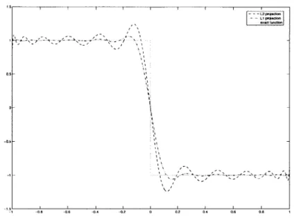
The implementation of the dMSV methodology, which relies essentially on the Ger-mano identity, involves projections of the solution on various scales. In Fourier Galerkin and Discontinuous Galerkin contexts, these projections generate the so-called Gibbs phenomenon when the solution is discontinuous, introducing spurious high-frequency oscillations. In some cases, these oscillations may be large enough to affect the evaluation of the model term's parameters, and lead to undervalued (hence inefficient) viscosities.
One possible way to mitigate the Gibbs phenomenon is to take a projection oper-ator that is more suited to the discontinuities of the solution than the plain L2 norm projection operator. The following plot shows two different projections of the "step" function f(x):
f(x)
1, if X < 0-1, if Lg> 0
0.5',
00.5
-- -0!s -0!6 -d4 _-12 o 042 04.1 0!6 0+s
Figure 3-1: Projections of the step function on (Li)io,...,25
This simple example shows how the L1 projection can be used to reduce the amplitude of the Gibbs oscillations. As we will see it later, we will make extensive use of this projection in one of the test cases we ran. The methodology for the computation of L1 projections will be detailed further in the chapter.
3.3.2
1-viscosity and 2-viscosity model terms
This section will describe the model terms we chose to implement in our shock-capturing algorithm and give more general insights on the way multi-parameter model terms are to be constructed.
1-viscosity model term
The first model term we implemented is the simple 1-viscosity model term. This term is of diffusive nature and its weak form can be written:
The corresponding one-dimensional Local Discontinuous Galerkin representation is:
M(vh uh h h hsYi) Tf qh(Vh
(3.11)
q fTr, LI''L ' dx =
uh'Lj'
-h
dxwith the fluxes:
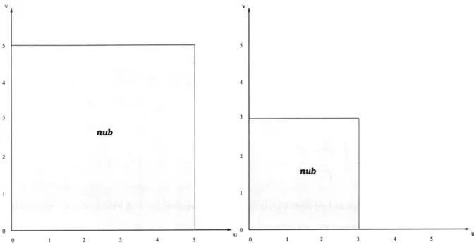
This model term has essentially been implemented for the validation of the method. As we will see later, its performance is not as high as that of more elaborated model terms and its main advantage relies on the relative simplicity of its LDG formulation. We will now introduce a useful way of representing on which moments of the solution uh and of the test function vh the artificial viscosity is acting. Let us consider two axes representing the Legendre moments of the solution uh (x-axis) and the test function vh (y-axis). Given a fifth-order space U(h and the third-order subspace Ul1
(we need two scales to close the system), in our 1-viscosity model term, the parameter -9 is acting on the following squares:
V
nub
2 2
nub
0 1 2 3 4 5 0 1 2 3 4 5
Figure 3-2: domains affected by the artificial viscosity V at scales 5 (right) and 3 (left)
In this case, the artificial viscosity P acts on every moment of the solution or
the weighting function so its representation is straightforward. For more complicated
model terms however, these plots give very valuable insights on whether or not these
model terms fit within the dMSV framework.
2-viscosity model term
The goal of multiple-parameter model terms, such as our proposed 2-viscosity model
term, is to introduce a separation of the modes of the solution, to group them and, to
assign a different viscosity to each group. As we will see it in the next chapter, this
increased complexity in the dMSV formulation is more than offset by the achieved
shock-capturing performance.
If
PL2Jdenotes the projection over the subspace
U1and I the identity function
then the weak form of our proposed 2-viscosity model term is:
M(v,u,s, ,) = - j Au - v dx - ijA( - PLPJ)
u.
(- pL2J)v
dx (3.12)high-order Legendre polynomials (Li, i > [2]) and the ones that correspond to lower-high-order Legendre polynomials (Li, i <
[f]).
Each of these two groups of moments has a different behavior near discontinuities. As a result, we are expecting better shock-capturing capabilities by assigning a specific artificial viscosity to each of them. The one-dimensional Local Discontinuous Galerkin formulation for this 2-viscosity model term is as follow:- h+h+2
M~vhuh~,~,) =.q([.v] -fh~k(v).,dx)
.- 2
-([.(]I - IPL)]2 ' fh [(RI pP)v] xdx)
The auxiliary quantities q and = being:
-h'+!
7 ' fT Lj L,4' dx = [uhL' h'-
f'
uh'( Lj') dx12
qj,
f L>"L>, dx =([-
R
PlJ)uh"L,"" -fh,,('
- PLhiRh" (L') dx- h" _
and the fluxes:
Uh' - Uh'
(If - IPLJ)Uh" = (If - IPLuJ)Uh"
qh - h
h =h
q = +
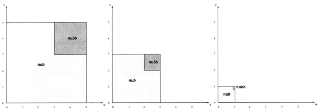
With a 2-viscosity model term, three different scales are needed to form enough con-sistency conditions to close the system. Given a fifth-order space U1, the following two subspaces: U3 and 1 can be used as scales in the generalized Germano indentity (3.8) to determine T7 and -. In which case, the domains affected by each parameter at each scale are:
I I__
1
nubb0 1 2 4 4 5 U 0 1 2 3 4 5 2 . 2 3 4 5
Figure 3-3: domains affected by the artificial viscosities TJ
and TV
at scales 5 (right), 3
(middle), and 1 (left)
Two remarks can then be made about this model term:
" Our proposed 2-viscosity model term is a generalization of the 2-viscosity model
term proposed by Oberai and Wanderer in [9] to a context in which the
space-differentiation and the projection operators do not commute and in which the
derivatives of the basis functions do not have any orthogonality relationship.
" It illustrates the fact that, when dealing with multi-parameter model terms,
the subspaces that will be used to derive the consistency conditions cannot be
arbitrary. In our example, the modes are equally divided into two groups and
this division is to remain the same for every scale on which the model term
is to be applied. For example, choosing
U4would have led to an unbalanced
partition of the moments between the two groups and must therefore be avoided
since it may lead to an incorrect evaluation of the parameters - and v.
The choice of a multi-parameter model term is therefore constrained by the
structure of the model term itself, which has to be consistent at every scale
on which the term will be applied. This consistency requirement reduces the
number of scales that are actually available to write the Germano identities,
as we showed it in the preceding paragraph. The reduced number of scales
available reduces in turn the number of possible parameters in the model term.
3.3.3
Projections
Writing the consistency conditions for the model term's parameters involves projec-tions on Legendre basis of various dimensions. Several projection operators can be used, but when Gibbs oscillations begin to develop, the choice of a specific projection operator has a direct impact on the performance of the algorithm. The purpose of this section is to present two projection operators that have been used in our dMSV routine.
L2 projection
The L2 projection is straightforward with our choice of a normalized Legendre basis on each element of the DG discretization. The L2
projection operator Pm is defined by:
P: --
,
p;>m+1Pm(Lh){0
if i>m+1Lh if i < m
Although very simple to implement and inexpensive, the results given by this L2 projection are subject to the Gibbs phenomenon. In certain cases, another projection operator, such as the L1 projection operator, which be detailed in the next section, will be needed to achieve a correct evaluation of the parameters.
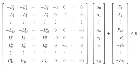
L1 projection
Let us consider a known function f defined over [-1, 1] and P, = 'O aiLi its L1 projection over the space of polynomials R., [X]. Then the L' projection is defined by the ai, which are such that the quantity (which represents the L1 norm of
f
- P,)is minimized:
This equation is then turned into a Linear Programming problem and solved.
If we divide the interval [-1, 1] into M equal subinterval, the integral (3.13) can be approximated by the following expression, with h = -2, Fm = hF(xm), L' = hL'(xm) and xm = 2Z- - 1: M M E |F(xm) - Pn(xm)|h = E m=1 m=1 n
|Fm
-E
aiL LI
i=o
whose associated Linear Programming problem is: Find ao, ... , a, T1, ... , TM such that:
M
min E Tm
m=0
under the constraints:
F1 - E 0aiL' F2 - E 0 iL' FM - E a -TM K TM < F1 -
En_
a~<F2
-- Ean FM - EOLwhich, in turn, can be written more conveniently in the following matrix form:
n+1 M
under the constraints:
-LO
-LI
-LO
-L'
-LO -L' LO LILO
L'
-1 0 ...0
0
-1 ... 00
0
...-1
-1
0
0
0 -1 ... 00
0
---
-1
3.3.4
Algorithms structure
Regardless of which model term is used, our dMSV algorithms all have a common
structure, which is presented in the following figure:
Moments (1)
Parameters (7)
Figure 3-4: dMSV algorithms structure
+
F
1 F2 FM-F
1-F
2 -FM<0
T2 TM --- Ln - -1- ; - - -L" n -- 2i -- ni --- Lnywhere:
1. The moments of the solution over the whole domain are given as inputs to the algorithm. Our implementation used a Runge-Kutta time-marching scheme; the tests showed that it is usually unnecessary to run the algorithm at each stage of the Runge-Kutta scheme.
2. The LDG auxiliary variables (i.e. the variables q) are computed. The number of auxiliary variables needed are directly linked to the structure of the model term.
3. The moments have to be projected on different scales during the parameter evaluation process, and it usually does make sense to compute these projec-tions at the beginning of the algorithm since they will be used in (2), (4) and (5). When straightforward projections are used, such as the L2 projection, the gain is not significant, but it becomes important when the computation of the projection is expensive, for example when
L
projections are used.4. The various quantities involved in the consistency conditions are evaluated, leaving the model term parameters as unknowns.
5. The time-derivative terms that are evaluated by computing the Discontinuous Galerkin residuals of the solution at the corresponding scales.
6. The linear system derived from the consistency conditions is solved.
Chapter 4
Results
In this chapter, the numerical results that have been obtained using the previously de-scribed Dynamic Multiscale Viscosity methodology are presented. Two model terms have been tested, the first one involving only one parameter and the second one in-volving two artificial viscosities. Regardless of which model term is used, we achieved optimal accuracy in the case of smooth solutions. The shock-capturing capability of each model term will also be discussed.
4.1
1-viscosity model term
The procedure presented in the section uses the simple 1-viscosity model term (3.11). The Runge-Kutta discontinuous Galerkin scheme is built upon fifth-order elements and a fourth-order time marching algorithm.
For the derivation of the consistency conditions and the evaluation of the artificial viscosity, the
L
projection operator presented in the preceding chapter, the scalesR [X] Rh
[X]
and the dissipation method have been used.4.1.1
Smooth solution
The first test aimed at determining whether the accuracy of the Runge-Kutta Discon-tinuous Galekin scheme was affected by the presence of a model term, in the case of a
smooth solution. To do so, we considered the one-dimensional linear transport equa-tion, to which we added the 1-viscosity model term (3.11) presented in the preceding chapter.
oj
9 h Vh dx +
f
h vh dx + M(Vh,u, s,) = 0
a t
a z
with the initial condition: u(x, 0) =
+
sin(wrx) and periodic boundary conditions.Iterated up to t = 1- , the numerical solution is then compared to the analytical one. The L2
norms of the errors are shown in the table below for various mesh sizes: number of elements 20 30 40
1e|
IL2 5.366236E-8 4.418526E-9 9.367500E-10Table 4.1: L2
error for the transport equation with a smooth initial condition and a 1-viscosity model term
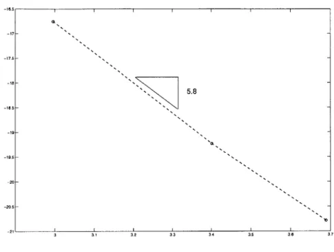
These results are used to compute the rate of convergence of the scheme. The rate of convergence of the procedure is presented on the figure below, the x-axis of the plot corresponding to the logarithm of the number of elements in the grid and the y-axis to the logarithm or the error:
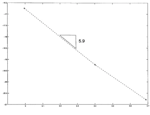
![Figure 4-2: iterated solution (top) and artificial viscosity evolution (bottom) over the time period [0, lf]for Pe=100](https://thumb-eu.123doks.com/thumbv2/123doknet/14754254.581719/50.918.224.711.139.926/figure-iterated-solution-artificial-viscosity-evolution-time-period.webp)
![Figure 4-3: iterated solution (top) and artificial viscosity evolution over the time period [.5 4] (bottom) for Pe=+inf](https://thumb-eu.123doks.com/thumbv2/123doknet/14754254.581719/51.918.194.680.147.930/figure-iterated-solution-artificial-viscosity-evolution-time-period.webp)
![Figure 4-5: iterated solution (top) and artificial viscosities evolution over the time period [0, -] (bottom) for Pe=5](https://thumb-eu.123doks.com/thumbv2/123doknet/14754254.581719/55.918.197.679.148.924/figure-iterated-solution-artificial-viscosities-evolution-time-period.webp)
![Figure 4-6: iterated solution (top) and artificial viscosities evolution over the time period [0, 9] (bottom) for Pe=10](https://thumb-eu.123doks.com/thumbv2/123doknet/14754254.581719/56.918.228.711.139.922/figure-iterated-solution-artificial-viscosities-evolution-time-period.webp)
